Utility Factor Curves for Plug-in Hybrid Electric Vehicles: Beyond the Standard Assumptions

Abstract

The utility factor (UF) of a plug-in hybrid electric vehicle (PHEV) refers to the ratio of miles traveled in electric mode to the total miles traveled. Standard UF curves provide a prediction of the expected achievable UF by a PHEV given its all-electric range (AER), but such predictions entail assumptions about both the driving patterns (distance traveled and energy intensity) and charging behavior. Studies have attempted to compare the real-world UF achieved by PHEVs to their standard values, but deviations can stem from deviations in assumptions about: (i) achievable electric range, (ii) travel distance and (iii) charging frequency. In this paper, we derive analytical models for modified utility factor curves as a function of both AER and charging behavior. We show that average charging frequency is insufficient to exactly predict UF but can still estimate bounds. Our generalized model can also provide insights into the efficacy of PHEVs in reducing carbon emissions.

1. Introduction

Plug-in hybrid electric vehicles (PHEVs) have powertrains that combine the traits of battery electric vehicles (BEVs) and hybrid electric vehicles (HEVs). Driving energy in HEVs, much like conventional vehicles, comes from fuel that powers an internal combustion engine (ICE) [1], but HEVs also have electric motor(s) and batteries that can assist in powering the vehicle (or completely power for short periods) and/or recapture energy during deceleration. The distinguishing feature of PHEVs [2] compared to HEVs is having larger capacity batteries that allow the vehicle to travel appreciable distances, known as the all-electric range (AER), without turning on its ICE, plus the capability to charge the battery from grid electricity like BEVs.

PHEVs have two main modes of driving: charge depletion (CD), in which electric energy from the battery is the main source of power, and charge sustaining (CS), in which fuel for the ICE is the main source of power. The utility factor (UF) of a PHEV generally refers to the ratio of miles traveled in CD mode to its total miles traveled [3]. It is important to acknowledge that different configurations and designs of PHEVs exist [4], and that under certain conditions and/or some PHEV powertrain designs, CD mode can involve small amounts of fuel consumption [5]. However, the current work in this paper focuses on usage cases where fuel consumption in CD mode is mostly negligible. As such, within the context of this paper, CD mode can be interchangeably referred to as “EV mode” and CS mode as “HEV mode”.

Different standards exist [3,6,7] that aim at predicting the expected UF of a PHEV as a function of its AER, often presented as “UF curves”, with the most prominent of which being SAE J2841 [3]. Accurate prediction of the UF for a PHEV carries significant importance because the UF is often used as a simplified metric for estimating tailpipe carbon emissions and thus has implications for present-day and future regulatory policies. However, standard UF curves entail underlying assumptions that may not necessarily be met by real-world PHEVs. Several modeling studies [8,9,10] have attempted to assess the effect of different drive patterns than those in SAE J2841, while other studies [11,12,13] have compared standard UF values with those that could be inferred from real-world PHEV data. As discussed in [12,13] and illustrated in Figure 1, three main categories of reasons why real-world UF may not align with standard UF curves include mismatches in assumptions about: (i) attained AER, (ii) actual travel distance and (iii) charging frequency.

While examining the illustration in Figure 1, a number of considerations ought to be kept in mind:

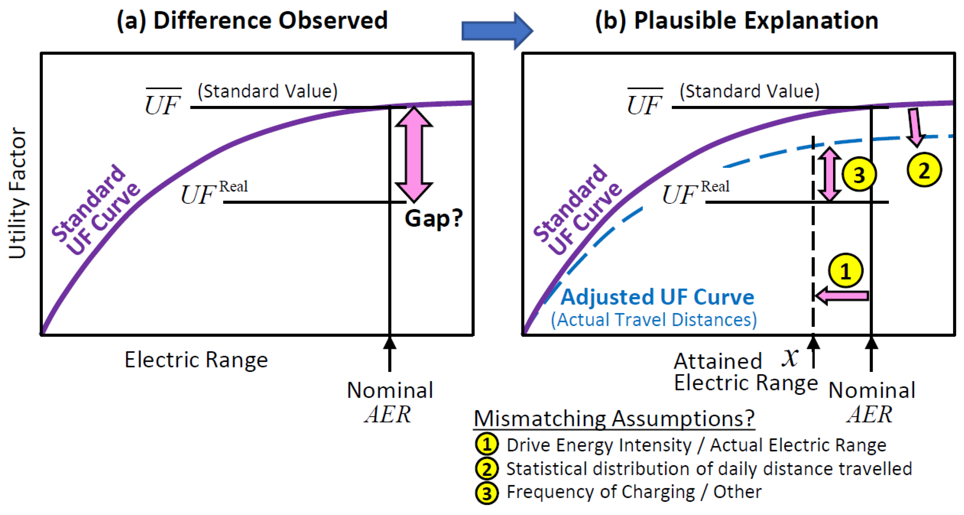
• The gap between standard and real UF values (Figure 1a) as well as the categories of reasons 1–3 (Figure 1b) were drawn in the “negative” direction (i.e., real UF being less than the standard UF). However, this is primarily for illustrative purposes. In reality, it is plausible for any of the three categories of reasons or the overall gap to be in either the positive (i.e., better UF than the standard rating) or negative directions.
• Each of the three main categories of reasons may include several sub-reasons; for example, category #1 (real-world attained AER) could be affected by the acceleration rate and speed driving style of vehicle owners, ambient temperature (which in turn affects both the efficiency of the electric powertrain as well as the heating/cooling power consumption for climate control of the passenger cabin), weight of passengers and cargo, gradient of the terrain (uphill/downhill), or towing load.
• It is also important to note that those three categories of reasons, while understood to be the main contributors to the UF gap, are not the only contributing reasons, nor is it necessarily true that they are linearly independent. For example, some PHEV designs may utilize electric power to warm up the battery during a cold climate, while others might utilize an alternative approach such as briefly turning on the engine, which in turn might affect the observable miles traveled in CD or EV mode.
• The (real-world) attained AER is not necessarily a static number like the nominal AER that is published by regulatory agencies such as the US EPA [14]. In fact, the attained AER can change from day to day depending on the vehicle usage conditions, and such daily variations in the attained AER can have interactions with the other two categories of reasons (charging frequency and distance traveled). Nonetheless, to avoid over-complicating the problem, secondary interactions between the reasons and “all other/unknown” reasons are often lumped with one of the three main categories of reasons.

While the SAE J2841 standard [3] has laid out the methodology for deriving UF curves from any dataset that provides a statistical distribution of vehicle miles traveled per day, the “standard UF values” quoted in the literature (such as [8,9,12,13]) often refer to the UF curves shown in [3], which were derived from the vehicle daily miles traveled profile in the 2001 National Household Travel Survey (NHTS-2001) [15]. Several studies [6,8,9,10] have shown alternative UF curves for different datasets of real-world vehicle miles traveled, and in particular, Paffumi et al. [10] considered models for additional daytime charging, thereby relaxing the typical assumption of “exactly once-only charging event (to full) before every drive day” in [3].

To the best of the authors’ knowledge, the current work in this paper is the first of its kind at attempting to lay out mathematical formulations for relaxing the typical once-only per drive day assumption to cases where the charging frequency is less than once per drive day. Similar to previous work [10], when considering charging frequencies different than exactly once per drive day, other assumptions come into play that result in a “family of plausible UF curves”, for which we also propose mathematical models that estimate the upper and lower bounds. Aside from cases of charging frequencies less than once per drive day, we also propose mathematical models for plausible bounds on UF curves when the charging frequency is more than once per drive day. The outcome from the extended families of UF curves can then serve as a means of gauging the carbon emissions reduction benefit via PHEVs under a broader set of usage conditions.

This paper started with a brief overview of relevant literature as well as a framing of the scope and motivation for the current work. The rest of the manuscript is organized as follows: Section 2 provides details of the mathematical models, along with examples of corresponding UF curves that illustrate how the curves change with various changes in assumptions. Section 3 provides a more in-depth discussion of the findings, along with some estimates of carbon emission reduction benefits. The manuscript then concludes with some highlights of key findings and expected future work directions.

2. Mathematical Model

2.1. Notations and Assumptions

Similar to the SAE J2841 standard [3], the primary input to the mathematical model is a dataset for daily miles traveled by a sample of vehicles. Vehicles in the dataset don’t necessarily need to be PHEVs or any particular type of powertrain, and as such, the methodology in [3] does not require any real-world charging information to be available in the dataset. In [3], UF for a hypothetical PHEV is calculated with the assumption that it would drive the same miles traveled profile, with a charging frequency of exactly one full charge before every drive-day (which we will denote as λ = 1) and no charging during daytime (which we will denote as μ = 0). Section 2.2 in this manuscript will derive mathematical models for estimating the UF in cases when the charging is less than once before every drive day and no daytime charging (0 < λ < 1, μ = 0), while Section 2.3 will derive mathematical models for estimating the UF in cases when the charging is once before every drive day, plus some daytime charging (λ = 1, μ > 0). To be considered more closely representative of the real-world, the horizontal axis for such UF curves ought to be the real-world attained AER, which will be denoted by the symbol x. In such a setup, it is also implicitly assumed that “all other/unknown” reasons for the UF gap are lumped with the Figure 1b category of reasons #1 (attained AER).

To better streamline the UF calculations in the mathematical model, for every vehicle sample i (i = 1 to N), the statistical profile for daily miles traveled is discretized and represented as a matrix of the number of driving days per year D_ij, with the first index (i) referring to days of travel by a certain vehicle, while the second index j refers to a range of miles traveled per day, depending on a discretization parameter δ. For example, if δ = 0.5 miles, then j = 10 refers to the range between 4.5 and 5.0 miles per day of travel distance. In this paper, we utilize the 2010–2012 California Household Travel Survey (CHTS) dataset [16], from which the matrix D_ij has been extracted. To make it easier to replicate the work in the current paper, a copy of the matrix D_ij has been placed in shared/public-accessible cloud storage [17]. Assuming the discretization parameter (δ), which was chosen at 0.5 miles, provides sufficient resolution, the annual miles traveled (l_ij) by a vehicle sample i on days with daily miles between (j − 1)δ and jδ is estimated (using upper bounds for daily miles interval) via Equation (1) as follows:

$$l_{ij}=D_{ij}\cdot \delta \cdot j$$

(1)

It follows that the total annual miles traveled by a vehicle (L_i) and the probability density mass for a fraction of the vehicle’s miles traveled (p_ij) on days with daily miles between (j − 1)δ and jδ can be calculated as:

$$L_i={\displaystyle \sum _{j=1}^J{l}_{ij}}$$

(2)

$$p_{ij}=\frac{l_{ij}}{L_i}$$

(3)

where J is the maximum number of discretized bins of miles per day of travel. In the current work, with δ = 0.5 miles, J was set at a value of 2000, which means that days with more than 1000 miles of travel (very rare occurrences in the CHTS dataset) were treated as if they were days with 1000 miles of travel.

A reference ${\overline{UF}}_i$ value, conforming to the charging behavior assumptions of [3] (i.e., λ = 1, μ = 0), can then be calculated for each vehicle sample given the real-world attained AER (x) as:

$${\overline{UF}}_i(x)={\displaystyle \sum _{j=1}^J{p}_{ij}\left(\frac{\min (x,\delta \cdot j)}{\delta \cdot j}\right)}$$

(4)

In order to go from calculating a UF value for each vehicle in the dataset to a population-wide estimate, SAE J2841 defines two different UF metrics [3]: (i) multi-day individual utility factor (MDIUF) and (ii) fleet utility factor (FUF). Simply put, MDIUF is a “simple average” of the UF values calculated for each vehicle in the dataset, while FUF effectively weighs each vehicle in the dataset by its total miles traveled. The purpose and usage of the two metrics are different. While MDIUF represents the expected value of UF for a randomly drawn sample vehicle, FUF, on the other hand, is an estimate of the total fraction of miles traveled by all vehicles that can be electrified. Furthermore, some datasets (CHTS included) can have representative weights for each of the vehicle samples that are often based on household demographics [18], so weighing each sample by its representative weight (w_i) effectively scales it up to the population that the dataset is intended to represent (all of California in the case of the CHTS dataset). The calculation of MDIUF and FUF can thus be performed as follows:

$$\overline{MDIUF}(x)=\frac{1}{W}{\displaystyle \sum _{i=1}^N{w}_i\cdot {\overline{UF}}_i(x)}$$

(5)

$$\overline{FUF}(x)=\frac{1}{Y}{\displaystyle \sum _{i=1}^N{L}_i{w}_i\cdot {\overline{UF}}_i(x)}$$

(6)

where W and Y are respectively the sum of vehicle sample weights and total weighed miles traveled, calculated as:

$$W={\displaystyle \sum _{i=1}^N{w}_i}$$

(7)

$$Y={\displaystyle \sum _{i=1}^N{L}_i{w}_i}$$

(8)

For datasets that don’t have vehicle sample weights, the typical assumption is to treat all vehicles equally (i.e., by setting all w_i = 1 in Equations (5)–(7)). For illustration purposes, the reference MDIUF and FUF curves (per Equations (5) and (6)) for the CHTS dataset are plotted in Figure 2 for the range of real-world attained AER (x) between 0 and 100 miles. Also shown in Figure 2 are the reference values from SAE J2841 [3] that are based on NHTS-2001. One notable observation in Figure 2 is that the reference UF curves (both MDIUF and FUF) via CHTS seem to have larger UF numbers than the reference UF curves via NHTS-2001 at any given value of x. This implies that the recorded vehicle travel in CHTS generally had fewer miles per drive day than in NHTS-2001. One plausible explanation for this could be the timing of data collection, where CHTS (data collected between 2010 and 2012) could have been affected by the 2008–2009 recession period in the US. Another plausible explanation could be due to the method of data collection, where NHTS-2001 utilized self-reported trip length data, while CHTS data utilized in this paper came from on-board device (OBD) logging of the sample vehicles. However, regardless of what dataset is used, the mathematical modeling approach in this paper could still be applied.

2.2. Charging Frequency Less Than Once per Drive Day

2.2.1. Overview

As a note, when considering mathematical modeling for charging frequency less than once per drive day, we are specifically referring to the case where the overnight charging before every drive day is less than once per day (i.e., 0 < λ < 1) and there is no daytime charging. To reduce clutter, we no longer mention daytime charging, but it should be understood that it is assumed that (μ = 0) within Section 2.2. It also ought to be noted that while λ is assumed to be strictly greater than zero and strictly less than 1, this is only to exclude the trivial case of λ = 0, for which UF is zero, and the case of λ = 1, for which UF can be calculated via Equations (5) and (6). Before building a mathematical model that addresses the fully general case of (0 < λ < 1), we first consider a few special cases.

2.2.2. Special Case: Binary Charging Behavior

This special case considers a mathematical model where the charging frequency for each individual vehicle in the data set (λ_i) can only take a value of either 0 or 1. In other words, while the overall average for the population of vehicles (λ) is between 0 and 1, this average is only attained via one set of vehicles (A) always charging (i.e., λ_i = 1, i ∈ A), while some vehicles are never charging (i.e., λ_i = 0, i ∉ A). This can be mathematically expressed as:

$$U{F}_i^{Bin}(x)={\lambda }_i\cdot {\overline{UF}}_i(x)$$

(9)

$$\lambda =\frac{1}{W}{\displaystyle \sum _{i\in A}{w}_i\cdot {\lambda }_i}$$

(10)

where $U{F}_i^{Bin}$ is the UF value for vehicle i with binary charging behavior, while ${\overline{UF}}_i$ is the reference UF value, computed via (Equation (4)). When considering going from UF values for each vehicle (per Equation (9)) to MDIUF and FUF estimates, it can make a big difference to the UF, which vehicles are in the set (A). As such, it is possible to estimate an expected value with the assumption of independent likelihood (i.e., any vehicle in the dataset is equally likely to be in the set A), as well as upper and lower bounds.

Expected Value with Independent Likelihood: when every vehicle in the dataset is equally likely to be in set (A), it can be shown that the UF for each vehicle i reduces to its reference UF value multiplied by the population average charging frequency (λ), which in turn allows for computing MDIUF and FUF as:

$$MDIU{F}^{Bin,Ind}(x)=\lambda \cdot \overline{MDIUF}(x)$$

(11)

$$FU{F}^{Bin,Ind}(x)=\lambda \cdot \overline{FUF}(x)$$

(12)

Upper and Lower Bounds: to compute upper and lower bounds for MDIUF and FUF, we setup optimization problems for maximizing/minimizing UF values with “which vehicles are in the set A” (i.e., which vehicle samples have corresponding λ_i = 1) as the decision variables. The optimization problem has the form:

$$\mathrm{For}\mathrm{MDIUF}:\mathrm{Minimize}/\mathrm{Maximize}{f}_{MDIUF}^{Bin}(x)=\frac{1}{W}{\displaystyle \sum _{i=1}^N{\lambda }_i\cdot w_i\cdot {\overline{UF}}_i(x)}$$

(13)

$$\mathrm{For}\mathrm{FUF}:\mathrm{Minimize}/\mathrm{Maximize}{f}_{FUF}^{Bin}(x)=\frac{1}{Y}{\displaystyle \sum _{i=1}^N{\lambda }_i\cdot w_i{L}_i\cdot {\overline{UF}}_i(x)}$$

(14)

$$\mathrm{Subject}\mathrm{To}:\frac{1}{W}{\displaystyle \sum _{i=1}^N{w}_i\cdot {\lambda }_i}=\lambda$$

(15)

$${\lambda }_i\in \left\{0,1\right\}$$

(16)

As a note, this optimization setup has the form of a linear program [19] (objective and constraints are linear in the decision variables λ_i), with all other quantities in Equations (13)–(15) being constant or possible to pre-compute before running the optimization problem to determine the upper/lower bounds for MDIUF or FUF. However, in the case of binary charging behavior, it is an integer-linear program (per the constraint in Equation (16)). While a generic integer linear program can be challenging to solve, when the number of vehicle samples in the dataset is sufficiently large, the equality constraint in Equation (15) can be satisfied within reasonable tolerance while relaxing the optimization problem to only solve its linear program version. The results of this model (independent, upper and lower bounds) for λ = 0.5 are shown in Figure 3a.

2.2.3. Special Case: All Vehicles with the Same Charging Frequency

This special case considers a mathematical model where the charging frequency for each individual vehicle in the data set (λ_i) is exactly equal to the charging frequency of the population average (λ). In other words, this is a case where all vehicles in a population are behaving exactly the same in terms of frequency of charging. For this special case, going from vehicle UF to population MDIUF and FUF is fairly straight-forward (similar to Equations (5) and (6)) as:

$$MDIU{F}^{Same}(x)=\frac{1}{W}{\displaystyle \sum _{i=1}^N{w}_i\cdot U{F}_i^{Same}(x,{\lambda }_i)}$$

(17)

$$FU{F}^{Same}(x)=\frac{1}{Y}{\displaystyle \sum _{i=1}^N{L}_i{w}_i\cdot U{F}_i^{Same}(x,{\lambda }_i)}$$

(18)

However, the calculation of UF for each vehicle sample as a function of its charging frequency (λ_i = λ) requires some further modeling assumptions. For this, we consider the calculation of an expected UF value based on an independent probability distribution for which days have a charging event before them, as well as upper and lower bounds.

Expected Value with Independent Probability: when considering a set of drive days by a vehicle sample i such that any drive day has an equal chance as any other drive day of having an overnight charging, the chance of a charging event becomes a Bernoulli experiment [20] with a chance of success equal to the overall average (which is λ_i = λ). Under such conditions, the UF of a vehicle sample can be expressed as:

$$U{F}_i^{Same,Ind}(x,{\lambda }_i)={\lambda }_i\cdot {\overline{UF}}_i(x)+{\lambda }_i(1-{\lambda }_i)\cdot {\overline{TDUF}}_i(x)+\dots$$

(19)

where the expression λ_i (1 − λ_i) that is multiplied by the second term in Equation (19) represents the probability of the current driving day not having a charging event after the previous driving day had a charging event. We don’t consider the rest of the terms after the second term in Equation (19) as they would be multiplied by λ_i (1 − λ_i)² (or even smaller numbers), so we consider them negligible compared to the first two terms. The equivalent UF for two days in a row after one overnight charging event is calculated as:

$${\overline{TDUF}}_i(x)={\displaystyle \sum _{j=1}^J\left(\frac{p_{ij}}{\delta \cdot j}{\displaystyle \sum _{k=1}^J{d}_{ik}\cdot \min \left(\delta \cdot j,\max \left(0,x-\delta \cdot k\right)\right)}\right)}$$

(20)

where d_ij is the probability density mass for vehicle i having a day with miles traveled within a certain range of miles per day:

$$d_{ij}=\frac{D_{ij}}{D_i}$$

(21)

$$D_i={\displaystyle \sum _{j=1}^J{D}_{ij}}$$

(22)

As a sanity check, one could confirm that the expression in (Equation (19)) converges to the same expression in (Equation (9)) as λ_i approaches a value of either 0 or 1.

Lower Bound: when considering a set of drive days by a vehicle sample, the temporal distribution of the charging events relative to driving days can have a significant effect on the attained UF. Generally speaking, when the charging events are mostly uniformly spaced, this results in better UF than non-uniformly spaced. For example, if λ_i = 0.5 with uniform spacing, this means that a charging event happens exactly one per two drive days, which can maximize utilization of each charging event. The opposite, least favorable temporal distribution is when/if all the charging events happen on back-to-back drive days while leaving a long gap of days without any charging events. Furthermore, if the stacked-up charging events are occurring before drive days that have the least contribution to attained electric miles, it would represent the lower bound for UF. To compute this lower bound, we set up an integer linear programming optimization problem similar to the setup in Section 2.2.2, but with the decision variables (v_j) controlling the temporal distribution of charging events.

$$\mathrm{Minimize}\hspace{1em}\hspace{1em}{f}^{Same,LB}(x,{\lambda }_i)={\displaystyle \sum _{j=1}^J{v}_{ij}\cdot p_{ij}\left(\frac{\min (x,\delta \cdot j)}{\delta \cdot j}\right)}$$

(23)

$$\mathrm{Subject}\mathrm{To}:\hspace{1em}\hspace{1em}\frac{1}{D_i}{\displaystyle \sum _{j=1}^J{v}_{ij}\cdot d_{ij}}={\lambda }_i$$

(24)

$$v_{ij}\in \left\{0,1\right\}$$

(25)

Upper Bound for λ_i = 0.5: in this estimate of an upper bound for UF, it is assumed that the temporal distribution of charging events is exactly evenly spaced at one charging event per two drive days, while being statistically independent from the number of miles traveled on any given day. The UF can then be calculated in a similar manner as Equation (19), but with the drive days either having a charging event or a charging event one day earlier (and no three or more drive days without a charging event):

$$U{F}_i^{Same,UB,Half}(x)=0.5\cdot {\overline{UF}}_i(x)+0.5\cdot {\overline{TDUF}}_i(x)$$

(26)

Upper Bound: For cases where λ_i < 0.5, we consider an upper bound for the UF via linear interpolation between zero and the upper bound value obtained from Equation (26). This corresponds to a temporal distribution of charging events where a portion of the time horizon has evenly spaced charging events at a frequency of one per two drive days, while the rest of the time horizon has no charging events. Likewise, for cases when λ_i > 0.5, we consider an upper bound for the UF via linear interpolation between the value obtained from Equation (26) and the case when λ_i = 1. This corresponds to a temporal distribution of charging events where a portion of the time horizon has evenly spaced charging events at a frequency of one per two drive days, while the rest of the time horizon has one charging event for every drive day. Combining the cases, the formula for the upper bound is summarized as:

$$U{F}_i^{Same,UB}(x,{\lambda }_i)=\left\{\begin{array}{c}2{\lambda }_i\cdot U{F}_i^{Same,UB,Half}(x)\hspace{1em}\hspace{1em}\hspace{1em}\hspace{1em}\hspace{1em}\hspace{1em}\hspace{1em}\hspace{1em}\hspace{1em}\hspace{1em}\hspace{1em}\hspace{1em}{\lambda }_i\le 0.5\hfill \\ (2{\lambda }_i-1)\cdot {\overline{UF}}_i(x)+(2-2{\lambda }_i)\cdot U{F}_i^{Same,UB,Half}(x)\hspace{1em}\hspace{1em}{\lambda }_i>0.5\end{array}\right.$$

(27)

The results of this model (independent, upper and lower bounds) for λ = 0.5 are shown in Figure 3b.

2.2.4. Generalized Upper and Lower Bounds

Given some value (λ) for the overall average frequency of charging, Section 2.2.2 highlighted plausible variations in UF by considering sensitivity to which vehicles within the population, while Section 2.2.3 highlighted plausible variations in UF by considering sensitivity to the temporal distribution of charging events relative to daily miles traveled by each vehicle. We now set up a set of more generic optimization problems, whose optimal solution provides the overall upper/lower bounds for MDIUF and FUF.

$$\mathrm{For}\mathrm{upper}\mathrm{bound}\mathrm{MDIUF}:\mathrm{Maximize}\hspace{1em}{f}_{MDIUF}^{Gen,UB}(x)=\frac{1}{W}{\displaystyle \sum _{i=1}^N{w}_i\cdot U{F}_i^{Same,UB}(x,{\lambda }_i)}$$

(28)

$$\mathrm{For}\mathrm{lower}\mathrm{bound}\mathrm{MDIUF}:\mathrm{Minimize}\hspace{1em}{f}_{MDIUF}^{Gen,LB}(x)=\frac{1}{W}{\displaystyle \sum _{i=1}^N{w}_i\cdot U{F}_i^{Same,LB}(x,{\lambda }_i)}$$

(29)

$$\mathrm{For}\mathrm{upper}\mathrm{bound}\mathrm{FUF}:\hspace{1em}\hspace{1em}\mathrm{Maximize}\hspace{1em}{f}_{FUF}^{Gen,UB}(x)=\frac{1}{Y}{\displaystyle \sum _{i=1}^N{w}_i{L}_i\cdot U{F}_i^{Same,UB}(x,{\lambda }_i)}$$

(30)

$$\mathrm{For}\mathrm{lower}\mathrm{bound}\mathrm{FUF}:\hspace{1em}\hspace{1em}\mathrm{Minimize}\hspace{1em}{f}_{FUF}^{Gen,LB}(x)=\frac{1}{Y}{\displaystyle \sum _{i=1}^N{w}_i{L}_i\cdot U{F}_i^{Same,LB}(x,{\lambda }_i)}$$

(31)

$$\mathrm{Subject}\mathrm{To}:\hspace{1em}\frac{1}{W}{\displaystyle \sum _{i=1}^N{w}_i\cdot {\lambda }_i}=\lambda$$

(32)

$$0\le {\lambda }_i\le 1$$

(33)

To calculate the upper or lower bounds for MDIUF or FUF, one needs to utilize the appropriate objective (among Equations (29)–(31)) along with the constraints in Equations (32) and (33). Though the constraints are linear and the decision variables are continuous (which generally makes the optimization problem easier to solve than integer programming), the objective functions, which include terms defined in Section 2.2.3, can have nonlinear terms in (λ_i), such as the terms defined via Equation (19) or even sub-optimization problems, such as when estimating lower bounds for an individual vehicle sample via Equations (23)–(25). As such, the optimization approach we tested for solving Equations (29)–(33) is the nonlinear programming technique known as successive linear programming [21]. The calculated upper and lower bound UF curves for λ = 0.5 are shown in Figure 3c.

A brief overview of the successive linear programming (SLP) optimization approach [21] is that it is a technique that attempts to find the optimum value within a solution domain of continuous variables (all λ_i in this case) for a nonlinear objective and/or constraints via solving a series of linear programming optimization problems. In each iteration of SLP, a linear approximation is constructed for the nonlinear objective and/or constraints (via function value and gradient at the “current solution” point). The linear approximation is then solved via linear programming techniques, with the solution of the linear programming becoming the new “current solution” point, and the process is repeated until convergence, which is typically when iterations of SLP can no longer find a better solution satisfying the problem constraints. In implementation for the current problem (solving for all λ_i), the constraints (Equations (32) and (33)) are actually linear, which means that the successive iterations of SLP always retain a feasible solution. Since the results of SLP, much like gradient-following optimization techniques, can be dependent on the “starting point”, a multi-start point strategy is employed, with two special cases (from Section 2.2.2 and Section 2.2.3) included among the starting points. This ensures that the solution returned by SLP (as shown in Figure 3c) is always “outside the envelope” of either of the two special cases (shown in Figure 3a,b).

2.3. Charging Frequency: More Than Once per Drive Day

There seems to be a perception that additional charging events beyond once per drive day tend to have diminishing returns. Part of this perception may come from some daytime charging events being limited by available time (e.g., charging a PHEV while the owner is shopping) and therefore not completely topping off the battery/restore full electric driving range. The other issue about daytime charging events is the timing relative to miles traveled on a given day. Even a top-off charging event may not add many electric miles if it happens too early or too late during a drive day. Furthermore, if a daytime charging event occurs on a day where the miles traveled are less than the electric range of the PHEV, there would be no “additional” electric miles on that day. As such, one may find corner cases where a lower bound on UF for (λ = 1, μ > 0) isn’t noticeably better than the reference case of (λ = 1, μ = 0). Thus, in this section, we focus more on plausible estimates of UF than minimum/maximum upper and lower bounds.

We develop mathematical models for the estimation of the UF factor for vehicles that charge to full before every drive day and gain a second full top-off charging event on some of the drive days, in other words, the case of (λ = 1, 0 < μ ≤ 1). We assume the daytime charging events have an independent probability of occurring (i.e., any drive day is equally likely to have a second charging event), which allows us to formulate a generic estimate of the UF of a sample vehicle as follows:

$$U{F}_i^{Daytime,Ind}(x,{\mu }_i)={\displaystyle \sum _{j=1}^J{p}_{ij}\left(\left(\frac{\min (x,\delta j)}{\delta j}\right)+{\mu }_i\left(\frac{\mathsf{\Phi }(\delta j)}{\delta j}\right)\right)}$$

(34)

where the function $\mathsf{\Phi }(\delta j)$ in the second term of Equation (34) represents the expected value for additional electric miles on a day with travel distance equal to ($\delta j$) due to the occurrence of a daytime charging event. The additional electric miles are a natural function of both the total miles traveled during that day as well as when the daytime charging event occurs and can be expressed as:

$$\mathsf{\Phi }(\delta j)=\left\{\begin{array}{c}0\hspace{1em}\hspace{1em}\hspace{1em}\hspace{1em}\hspace{1em}\hspace{1em}\hspace{1em}\delta j\le x\hfill \\ {\displaystyle \underset{y=0}{\overset{\delta j}{\int }}\varphi (y)\cdot g(y)dy}\hspace{1em}\hspace{1em}\delta j>x\end{array}\right.$$

(35)

$$\varphi (y)=\left\{\begin{array}{cc}\min (y,\delta j-x)& y\le x\\ x& x<y\le \delta j-x\\ \delta j-y& y>\delta j-x\end{array}\right.$$

(36)

where the function $g(y)$ is the probability density function for occurrence of the daytime charging event after how many miles (y) have been traveled. In demonstration of this model (as shown in Figure 4), we utilize the exponential distribution [20], which is a typical assumption for random arrivals in queueing systems. The distribution is also shifted such that the daytime charging event wouldn’t occur until half the electric range has been traveled, and the exponential parameter is set to have the average occurrence of the daytime charging event between half the electric range and the full electric range. We also note that Equation (34) can be used to estimate UF if all vehicles in the dataset had the same frequency for daytime charging (which we consider a plausible scenario), or μ_i can have binary (0 or 1) values and an integer linear optimization framework (similar to Section 2.2.2) can be applied to estimate upper and lower bounds, as shown in Figure 4.

2.4. Summary of Modelled Cases

A summary list of the modelled cases for charging behavior in this work is provided in

Table 1. Summary of Charging Behavior Modelled Cases.

Case	Discussed	Description
λi ∈ {0, 1}, μ = 0	Section 2.2.2	No daytime charging. Overnight charging behavior is binary; some vehicles always charge, others never charge.
All λi = λ, 0 ≤ λ ≤ 1, μ = 0	Section 2.2.3	No daytime charging. The overnight charging frequency is the same for all vehicles.
0 ≤ λi ≤ 1, μ = 0	Section 2.2.4	No daytime charging. Generalized case for overnight charging, where some vehicles always charge, some never charge, others somewhere in-between.
All λi = 1, 0 ≤ μi ≤ 1	Section 2.3	Vehicles always charge overnight. Some vehicles also gain one additional charging event during the day.
0 ≤ λi ≤ 1, 0 ≤ μi	Section 3, future work	Fully generalized case where overnight charging frequency for each individual vehicle can be anywhere between always and never, while at the same time, each individual vehicle may have additional one or more charging events during the day

. To further enhance the modeling perspective, it is noted that the actual timing of a charging event (during nighttime or daytime) isn’t what drives the mathematical model. Rather, a charging event (fully topping the electric range in the battery) between two drive days is the mathematical equivalent of an “overnight” charging event, while an “additional” charging event within a one-day window after a previous charging event is the mathematical equivalent of a “daytime” charging event. In which case, as long as there is no significant temporal overlap between the charging events, one may use the sum of λ and μ as a proxy estimator for the fully generalized case (as is performed in the discussion in Section 3). However, detailed derivation for the fully generalized case is beyond the scope of current work.

3. Discussion

British statistician George Box once famously wrote “All models are wrong, some are useful”. When one reflects on when the concept of UF and UF curves were originally being developed (with standard assumptions), one of the main appeal points was that UF curves were relatively “easy” to use and understand. However, when standard assumptions are called into question in order to create more realistic real-world behavior models, it becomes apparent that real-world UF observations can be affected by many complex details. Perhaps the primary contribution in this work is not so much the calculation of UF curves for various charging frequencies as it is bringing into focus how wide the difference between upper and lower bounds can be in some cases, as observed in Figure 4. It also ought to not be forgotten that the modeling work in Section 2.2 and Section 2.3 is still involving several simplifying assumptions, such as independent probabilities or consideration of daytime charging only after overnight charging before a drive day has been fulfilled, when in reality, some vehicle owners may not necessarily charge before every drive day, but they can still occasionally do daytime charging. It may be possible to further verify the degree of validity of such assumptions by comparing them with real-world PHEVs data, though this would require some much more detailed vehicle data than is typically available via public travel surveys. Such validation work is beyond the scope of the current paper.

Another issue about the concept of UF that is often ignored in favor of it being easy to use is that UF can be taken as a proxy estimate of only the tail-pipe emissions from a PHEV. In some instances, deviations in the real-world from ideal UF curves are being used as a reason to suggest lowering the regulatory carbon emissions reduction benefit of PHEVs [22,23]. However, this implicitly ignores the fact that electric miles also have equivalent carbon emissions depending on the fuel mix for electricity generation. What could be a more relevant metric for gauging the benefit of PHEVs is considering how much well-to-wheels [24] reduction of carbon emissions they can bring compared to an equivalent conventional vehicle. For a present-day scenario demonstrating such a concept, we use the EPA label values [14] for the 2022 RAV4 and RAV4 Prime (respectively at 29 MPG, 38 MPG in CS mode and 0.36 kWh/mile in CD mode), along with the 2021 average carbon intensity for the US electric grid at ~450 g-CO₂/kWh (calculated via fuel mix information from the US EIA [25] and GREET model [24]) and 10,778 g-CO₂/gal for E10 gasoline. We also consider scenarios for the year 2050 with projected carbon intensity for electricity at 180 g-CO₂/kWh, as well as 50% reduced carbon intensity for gasoline. Using plausible FUF values (from Figure 4b) at different charging frequencies, carbon emissions offset results for the considered scenarios are shown in Figure 5.

Considering the bigger picture of well-to-wheels analysis (Figure 5) can dramatically change the sensitivity of carbon emission reductions (relative to an equivalent conventional vehicle) to the charging frequency of PHEVs. In fact, at the present-day average US electric grid, the carbon emissions in CD mode (electric) miles are only about 25% less than the carbon emissions per mile traveled in CS mode on the E10 gasoline blend. While a 50-mile AER PHEV (scenario 1 in Figure 5) offsets about 37% of the carbon emissions of an equivalent conventional vehicle when charged exactly once per drive day, the same PHEV can still offset about 31% of the carbon emissions when its frequency of charging is 0.5 (once per two drive days on average). The difference between a 50- and an 80-mile AER PHEV also appears minimal in (scenario 1 Figure 5). With lower carbon intensity in the electric grid and no change in the gasoline blend (scenario 2 in Figure 5), the difference between 50- and 80-mile AER, as well as the sensitivity to charging frequency, becomes more pronounced. However, it also stands to reason that future liquid fuels would have an increased fraction of biofuels and/or carbon-capture/synthetic fuels that are lower in carbon intensity. In such cases (scenario 3 in Figure 5), it can still be an attractive option across a broad range of usage conditions.

4. Conclusions

This paper considered an extension of the standard assumptions for generating UF curves, with the aim of encompassing a broader range of realistic charging behavior by PHEV owners. Mathematical models were proposed that address a specific number of cases, as well as an optimization framework that can be utilized to estimate upper and lower bounds. Though UF is a fairly simple concept, it has the drawback of not being indicative of the bigger picture (such as well-to-wheels or full lifecycle) of carbon emissions. When considering well-to-wheels, it can be shown that the carbon emissions reduction benefits of a PHEV relative to an equivalent conventional vehicle are not very sensitive to the frequency of charging or longer than 50 miles AER unless the difference in carbon intensity between CD mode and CS mode is high (which doesn’t occur except with very low carbon electricity and high fossil content liquid fuels). Future extensions of this work may include comparison with detailed real-world PHEV data in order to gauge the realism of the various assumptions in the proposed mathematical models, as well as further extension of the mathematical model to consider the interaction/supplementation effects of daytime charging when overnight charging is less frequent than every night.

References

1. US Department of Energy. How Hybrids Work. Available online: https://www.fueleconomy.gov/feg/hybridtech.shtml (accessed on 16 November 2022).
2. US Environmental Protection Agency. Electric & Plug-In Hybrid Electric Vehicles. Available online: https://www.epa.gov/greenvehicles/explaining-electric-plug-hybrid-electric-vehicles (accessed on 16 November 2022).
3. Society of Automotive Engineers (SAE). J2841_201009: Utility Factor Definitions for Plug-In Hybrid Electric Vehicles Using Travel Survey Data; SAE International: Warrendale, PA, USA, 2010. [Google Scholar]
4. US Department of Energy. Plug-In Hybrids. Available online: https://www.fueleconomy.gov/feg/phevtech.shtml (accessed on 16 November 2022).
5. US Environmental Protection Agency. Explaining Electric & Plug-In Hybrid Electric Vehicles. Available online: https://19january2017snapshot.epa.gov/greenvehicles/explaining-electric-plug-hybrid-electric-vehicles_.html (accessed on 1 March 2023).
6. United Nations Economic Commission for Europe. United Nations Global Technical Regulation on Worldwide Harmonized Light Vehicles Test Procedures (WLTP). Available online: https://unece.org/fileadmin/DAM/trans/main/wp29/wp29wgs/wp29gen/wp29registry/ECE-TRANS-180a15am4e.pdf (accessed on 17 March 2023).
7. Liu, X.; Zhao, F.; Hao, H.; Chen, K.; Liu, Z.; Babiker, H.; Amer, A. From NEDC to WLTP: Effect on the Energy Consumption, NEV Credits, and Subsidies Policies of PHEV in the Chinese Market. Sustainability 2020, 12, 5747. [Google Scholar] [CrossRef]
8. Bradley, T.; Quinn, C. Analysis of plug-in hybrid electric vehicle utility factors. J. Power Sources 2010, 195, 5399–5408. [Google Scholar] [CrossRef]
9. Wu, X.; Aviquzzaman, M.; Lin, Z. Analysis of plug-in hybrid electric vehicles’ utility factors using GPS-based longitudinal travel data. Transp. Res. Part C 2015, 57, 1–12. [Google Scholar] [CrossRef]
10. Paffumi, E.; De Gennaro, M.; Martini, G. Alternative utility factor versus the SAE J2841 standard method for PHEV and BEV applications. Transp. Policy 2018, 68, 80–97. [Google Scholar] [CrossRef]
11. Smart, J.; Bradley, T.; Salisbury, S. Actual Versus Estimated Utility Factor of a Large Set of Privately Owned Chevrolet Volts. Int. J. Altern. Powertrains 2014, 3, 30–35. [Google Scholar] [CrossRef]
12. Raghavan, S.; Tal, G. Plug-in hybrid electric vehicle observed utility factor: Why the observed electrification performance differ from expectations. Int. J. Sustain. Transp. 2020, 16, 105–136. [Google Scholar] [CrossRef]
13. Hamza, K.; Laberteaux, K.; Chu, K.-C. On inferred real-world fuel consumption of past decade plug-in hybrid electric vehicles in the US. Environ. Res. Lett. 2022, 17, 104053. [Google Scholar] [CrossRef]
14. US Environmental Protection Agency. Fuel Economy Guide. Available online: https://www.fueleconomy.gov/feg/printGuides.shtml (accessed on 18 March 2023).
15. US Department of Transportation. National Household Travel Survey. Available online: https://nhts.ornl.gov/download.shtm (accessed on 18 March 2023).
16. National Renewable Energy Laboratory. 2010–2012 California Household Travel Survey. Available online: https://www.nrel.gov/transportation/secure-transportation-data/tsdc-california-travel-survey.html (accessed on 18 March 2023).
17. Utility Factors Extended (Data Available on Google Drive Cloud Storage). Available online: https://drive.google.com/drive/folders/1UL3FTffKbgbgi_EMVu0bWt_CQTkS2_hr?usp=sharing (accessed on 18 March 2023).
18. NuStats LLC. 2010–2012 California Household Travel Survey Final Report. Available online: https://www.nrel.gov/transportation/secure-transportation-data/assets/pdfs/calif_household_travel_survey.pdf (accessed on 19 March 2023).
19. Hu, T.; Kahng, A. Linear and Integer Programming Made Easy; Springer: Berlin/Heidelberg, Germany, 2016. [Google Scholar]
20. Collani, E.; Draeger, K. Binomial Distribution Handbook for Scientists and Engineers; Springer: Berlin/Heidelberg, Germany, 2001. [Google Scholar]
21. Bazaraa, M.; Sherali, H.; Shetty, C. Nonlinear Programming: Theory and Algorithms; Wiley: New York, NY, USA, 2006. [Google Scholar]
22. Plötz, P.; Moll, C.; Bieker, G.; Mock, P. From lab-to-road: Real-world fuel consumption and CO2 emissions of plug-in hybrid electric vehicles. Environ. Res. Lett. 2021, 16, 054078. [Google Scholar] [CrossRef]
23. US Environmental Protection Agency. Multi-Pollutant Emissions Standards for Model Years 2027 and Later Light-Duty and Medium-Duty Vehicles. 2023. Available online: https://www.regulations.gov/search?documentTypes=Proposed%20Rule&filter=EPA-HQ-OAR-2022-0829 (accessed on 23 October 2023).
24. Argonne National Laboratory. GREET Model. Available online: https://greet.es.anl.gov/ (accessed on 20 March 2023).
25. US Energy Information Administration. Available online: https://www.eia.gov/electricity/annual/ (accessed on 3 October 2023).
Figure 1. Illustration of three categories of assumptions mismatch between standard UF curves and real-world.
Wevj 14 00301 g001
Figure 2. Reference UF curves via CHTS and SAE J2841 (based on NHTS-2001).
Wevj 14 00301 g002
Figure 3. Reference UF curves and various models for λ = 0.5.
Wevj 14 00301 g003
Figure 4. Plausible and Upper/Lower UF curves for select modelled charging frequency.
Wevj 14 00301 g004
Figure 5. Select carbon emissions offset scenarios relative to an equivalent conventional vehicle.
Wevj 14 00301 g005