Assessment of an Electric Vehicle Drive Cycle in Relation to Minimised Energy Consumption with Driving Behaviour: The Case of Addis Ababa, Ethiopia, and Its Suburbs

Abstract

Battery electric vehicles (BEV) are suitable alternatives for achieving energy independence and meeting the criteria for reducing greenhouse emissions in the transportation sector. Evaluating their performance and energy consumption in the real-data driving cycle (DC) is important. The purpose of this work is to develop a BEV DC for the interlinked urban and suburban route of Addis Ababa (AA) in Ethiopia. In this study, a new approach of micro-trip random selection-to-rebuild with behaviour split (RSBS) was implemented, and its effectiveness was compared via the k-means clustering method. When comparing the statistical distribution of velocity and acceleration with measured real data, the RSBS cycle shows a minimum error of 2% and 2.3%, respectively. By splitting driving behaviour, aggressive drivers were found to consume more energy because of frequent panic stops and subsequent acceleration. In braking mode, coast drivers were found to improve the regenerative braking possibility and efficiency, which can extend the range by 10.8%, whereas aggressive drivers could only achieve 3.9%. Also, resynthesised RSBS with the percentage of behaviour split and its energy and power consumption were compared with standard cycles. A significant reduction of 14.57% from UDDS and 8.9% from WLTC-2 in energy consumption was achieved for the AA and its suburbs DC, indicating that this DC could be useful for both the city and suburbs.

1. Introduction

There has been a global increase in battery electric vehicles (BEVs) owing to their potential to offer emission-free, highly efficient, and safe transportation [1,2,3]. However, the primary obstacles to adopting e-mobility are the range anxiety associated with a long charging time and the high investment cost of charging stations [4]. To enhance the commercial market share of BEVs, the challenges of grid power forecasting, energy consumption estimation, and lifecycle analysis need to be addressed. Furthermore, BEV design must satisfy top-level customer attributes and requirements associated with dynamic performance and energy consumption. Accordingly, accurate calculation of driving range and energy consumption is a primary task in the predesign analysis of BEV powertrain and energy storage systems. For such predictions, the driving cycle (DC) has been widely utilised as an input parameter to track the road trajectory on a simulation platform [5]. Furthermore, DC is considered a standardised testing tool for certifying new designs and evaluating the performance of different types of vehicles.

In recent years, several extensive studies have been conducted on the development of standard and legislative DCs worldwide, targeting the testing and evaluation of engine emissions and fuel consumption. These include the United States of America’s (USA) Environmental Protection Agency (EPA-75), Urban Dynamometer Driving Schedule (UDDS), Federal Test Procedure (FTP-75), Highway Fuel Economy Test (HWFET), New York City Cycle (NYCC), the New European Driving Cycle (NEDC), and the Worldwide Harmonised Light Vehicles Test Cycle (WLTC), to mention a few [2,6].

As DC is a second-by-second speed and time profile that represents typical real-time driving patterns in a particular urban area and region, its characteristics differ between regions and cities. Such a driving pattern can be influenced by an individual’s driving behaviour and the interaction with the road traffic environment. However, driving behaviour information cannot be measured directly using driving profile parameters. Various methodologies have been presented to determine driving behaviour based on driving data. Author [7] used naturalistic driving data to identify driving style; refs. [8,9] presented different classifications of driving behaviour, such as aggressive, average, and mild. Some previous studies demonstrated the existence of a high correlation between the driving style, the acceleration, and the velocity of a cycle by introducing the possibility of a percentage of aggressiveness. Many studies have confirmed that aggressive driving styles record higher values of energy consumption than drivers driving calmly do. However, in most studied regional BEV DCs, the driving pattern has been characterised by focusing on the acceleration behaviour only and ignoring the braking behaviour [10,11]. Other studies have indicated the presence of significant differences in braking power intensity between aggressive and coast braking [12,13].

Researchers and automotive manufacturers have been using readily available standard and legislative DCs to evaluate and certify the design requirements of BEV [14,15,16]. However, this approach means that accurate estimation cannot be achieved as there are significant differences in torque, power, and braking characteristics of BEV and ICEV in a wide speed-operating range [17,18]. In recognition of the significant differences in standard and real-data DCs to determine country-specific energy consumption, different countries and automotive manufacturers have successfully developed the most realistic DCs that are unique to each city or region [19,20].

The techniques reported in most earlier studies for synthesising DCs are random selection, clustering, pattern classification, and modal analysis. Random selection is better for heterogeneous traffic conditions but requires exhaustive statistical analysis [21,22]. The pattern classification method is helpful for studying traffic patterns, but accurate measurement is difficult [21,23]. The cycles developed by the modal method, in which the Markov chain concept is implemented, fail to match real-data population parameters [24]. The k-means technique has the flexibility to deal with a variety of driving data but fails to represent real data accurately [22,25]. Furthermore, the cycles constructed by different methods are of varying duration, such as WLTC-3 (1800 s), Indian urban (2690 s), Sydney (637 s), WLTC-2 (1477 s), UDDS (1400 s), and Singapore (2344 s) [12]. The total duration of some regional DCs has been set to 1200–1300 s in order to simplify the simulation burden.

Almost all previous studies on the synthesis of BEV DCs have been based on data from road conditions in developed countries, with only a few contributions from developing countries such as India [22]. Very few studies [26], such as on Addis Ababa (AA), Ethiopian urban DCs, and [13] DCs for Egypt, have developed representative DCs for low-income countries, focusing on emission rates and fuel consumption estimation. However, as concluded by [17,18], these DCs could not be replicable for BEV evaluation and certification. Furthermore, in the development process of these cycles, the study area covered was only the urban territory, with no consideration given to the influence of suburbs on the inner city driving pattern and trip duration. In most capital cities of low-income countries such as AA, the driving pattern is influenced by roads’ mixed-use by pedestrians and different vehicles, single-lane vehicle composition, poor road quality and the absence of traffic signals [4,22]. As Ethiopia’s capital and the seat of the African Union (AU), AA is characterised by a comprehensive economic, political, cultural, and diplomatic environment, with varying topography, population dynamics, and highly congested traffic conditions. AA is a highly populated city with more than 5.23 million residents, and it is growing at a rate of 4.4% annually. The city has a total of around 630,000 registered vehicles, and the count along a single-lane asphalt road is 168 vehicles per kilometre [26]. AA is surrounded by small towns such as Bishoftu (east), Sandafa (north), Sululta (northwest), Holeta (west), and Sebeta (south), with 60 km of suburban routes from the city centre along cross-country main roads. Public transportation using city buses is preferred by most low-income people and extends to the five towns as destinations, starting from the central station (stadium), operating daily from 5.00 a.m. to 9.00 p.m. Furthermore, passenger cars are the preferred means of transport by those in the middle-income class living in AA and looking for low-cost accommodation in neighbouring towns [10].

To the authors’ knowledge, no investigations have yet been reported on the development of a BEV DC for a connected urban and suburban setting focusing on emerging large cities such as Addis Ababa (AA). Furthermore, the authors found that a single method was not sufficient to explore all essential driving features and behaviours in the regional driving profile. Therefore, the aim of this study was to assess country-specific low-energy consumption BEV DC based on Global Positioning System (GPS)-recorded real-time data from AA and its suburban (AASU) routes. This article proposes a new construction method that combines micro trip random selection-to-rebuild with behaviour split (RSBS) to synthesise an AASU representative DC. Thereafter, using the same data and k-means clustering method, another cycle was synthesised to compare its effectiveness and representativeness for regional data.

This approach can be used for both city and suburb driving cycles, considering driver behaviour to minimize energy consumption and increase the range of battery electric vehicles.

2. Materials and Methods

2.1. Route Selection

Routes were selected so as to represent typical driving patterns observed in the study area, considering home-to-work trips, population differences, and road classifications [26].

Accordingly, the inner city routes covering all types of routes and trip segments and extending to all five neighbouring towns were selected, marked in yellow in Figure 1a. The inner city road network is shown in Figure 1b. The longest route, which also features an expressway, stretches from AA to Bishoftu. Overall, this route is 59.8 km long and is comprised of a 19.8 km expressway, a 15.9 km suburban ring road and a 4.8 km feeder road, while the remaining 10.6 km and 8.7 km are the AA and Bishoftu inner city routes, respectively. City express bus manufactured by Yutong, China and passenger car of Toyota, Japan that were instrumented with GPS tracker of Itrack, India were used to collect data.

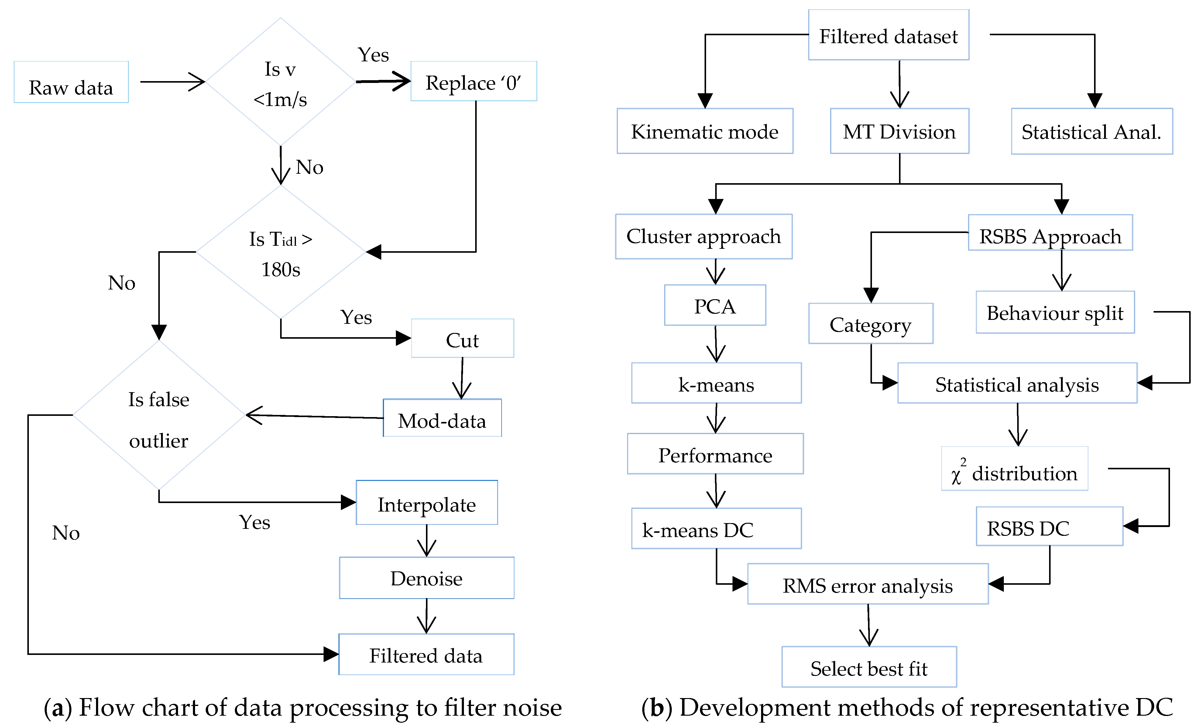
2.2. Data Collection and Processing

Initially, the driving profile data files were recorded by GPS at a frequency of 0.1 Hz using six vehicles, three from each passenger and city bus category. The collected raw data were filtered and denoised to minimise errors and to obtain smooth data and then concatenated into a unified dataset using MATLAB code, as shown in Figure 2a. Initially, a car speed below 1 m/s was changed to 0 m/s as its real applicability was insignificant, while speeds above 120 km/h were adjusted to the allowable maximum speed limit of 120 km/h. Next, data corresponding to the dwell time where vehicles stopped for a duration of more than 180 s were removed. Higher acceleration values due to a GPS error and sudden peaking speed were considered outliers. A void in speed values and alternating zero speed values may be recorded due to a GPS sensor defect or by being blocked by tall buildings [11,27]. The outliers of void and false data were treated using shape-preserving cubic interpolation, followed by the Bayes wavelet signal denoising method to smooth and transform to 1 Hz.

Finally, processed data equivalent to an approximate distance of 1390.47 km were determined for use in DC development methods, as shown in Figure 2b.

Table 1. Unified dataset before and after filtration process.

Data Type	Total Number of Data	Percentage of Data (%)
Raw data	179,894	100.00
Long dwell	14,724	8.18
Zero drift	900	0.50
False zero	200	0.11
Removed	15,824	8.80
Filtered	164,070	91.20

summarises the processed data, where zero drift and void are only 0.5% and 0.11%, respectively. A total of 8.18% of data was removed due to the long dwell time. The speed-acceleration distribution of the filtered and unified dataset can be seen in Figure 3.

2.3. Driving Feature Definition and Pattern Characterisation

Numerous studies have proposed different calculated parameters related to speed-acceleration distribution and time proportion in order to define driving features. They are categorised as level, distribution, and oscillatory measures.

However, there is no clear evidence of relevant parameters to predict the power and energy demand of a BEV. In this study, the 12 most prominent features with more variability and less of a relationship between them were selected after box plot statistical correlation analysis had been performed on 17 feature parameters presented in

Table 2. Driving features used to characterise Addis Ababa and its suburban driving pattern.

No.	Feature Category	Driving Features	Symbol
1	Level measures	Average speed (km/h)	Vave
2		Maximum speed (km/h)	Vmax
3		Average running speed (km/h)	Vrave
4		Average acceleration (m/s2)	aave
5		Maximum acceleration (m/s2)	amax
6		Average deceleration (m/s2)	dave
7		Maximum deceleration (m/s2)	dmax
8		Total duration (s)	Ttot
9		Approximated distance (km)	Dlng
10	Oscillatory measures	Relative positive acceleration (m/s2)	RPA
11		Positive aggressiveness index (m2/s3)	PAI
12		Relative negative acceleration (m/s2)	RNA
13		Negative aggressiveness index (m2/s3)	NAI
14	Distribution measures	Time percentage of idling (%)	Tidle
15		Time percentage of cruising (%)	Tcruz
16		Time percentage of acceleration (%)	Taccel
17		Time percentage of deceleration (%)	Tdecel

.

When characterising driving patterns, the impact of driving behaviour, mainly as a result of the driver’s driving style, must be included [28]. Although it is difficult to measure driving behaviour, there is a high correlation between driving style and acceleration-related feature parameters. Hence, acceleration-related features, including a_ave, d_ave PAI, NAI, RPA and RNA, were analysed to define different driving behaviours to characterise the driving pattern. RPA and RNA were considered principal components since they have a high correlation with the BEV energy consumption rate and the regenerative potential of braking kinetic energy per range, respectively [2,29,30]. RPA and RNA are defined as [31]

$$\mathrm{RPA}={\displaystyle \int \mathrm{v}\left(\mathrm{t}\right)\hspace{0.17em}{\mathrm{a}\left(\mathrm{t}\right)}^{+}}/{\displaystyle \int \mathrm{v}\left(\mathrm{t}\right)\hspace{0.17em}\mathrm{dt}}$$

(1)

$$\mathrm{RNA}={\displaystyle \int \mathrm{v}\left(\mathrm{t}\right)\hspace{0.17em}{\mathrm{a}\left(\mathrm{t}\right)}^{-}}/{\displaystyle \int \mathrm{v}\left(\mathrm{t}\right)\hspace{0.17em}\mathrm{dt}}$$

(2)

where V(t) is speed; a(t)⁺ is positive acceleration; a(t)⁻ is negative acceleration, and dt is the change in time.

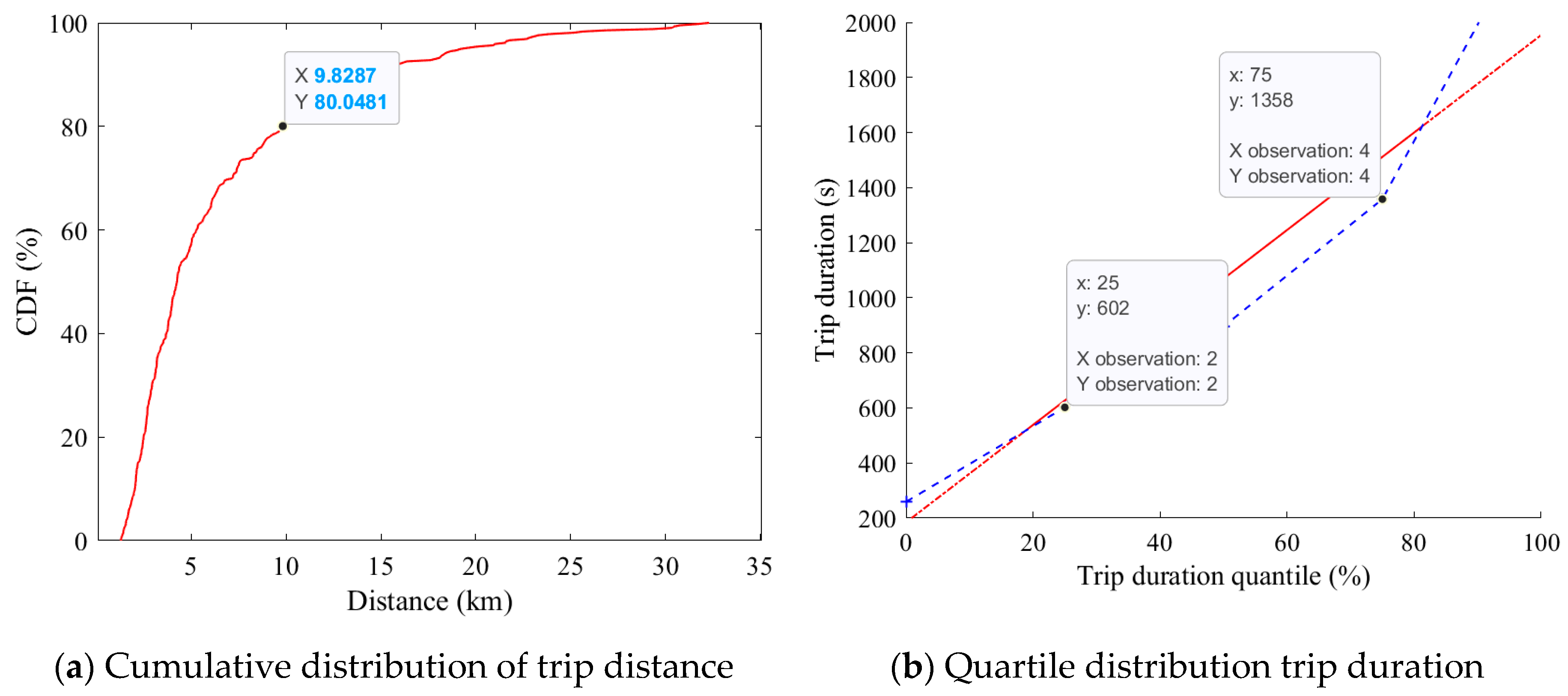
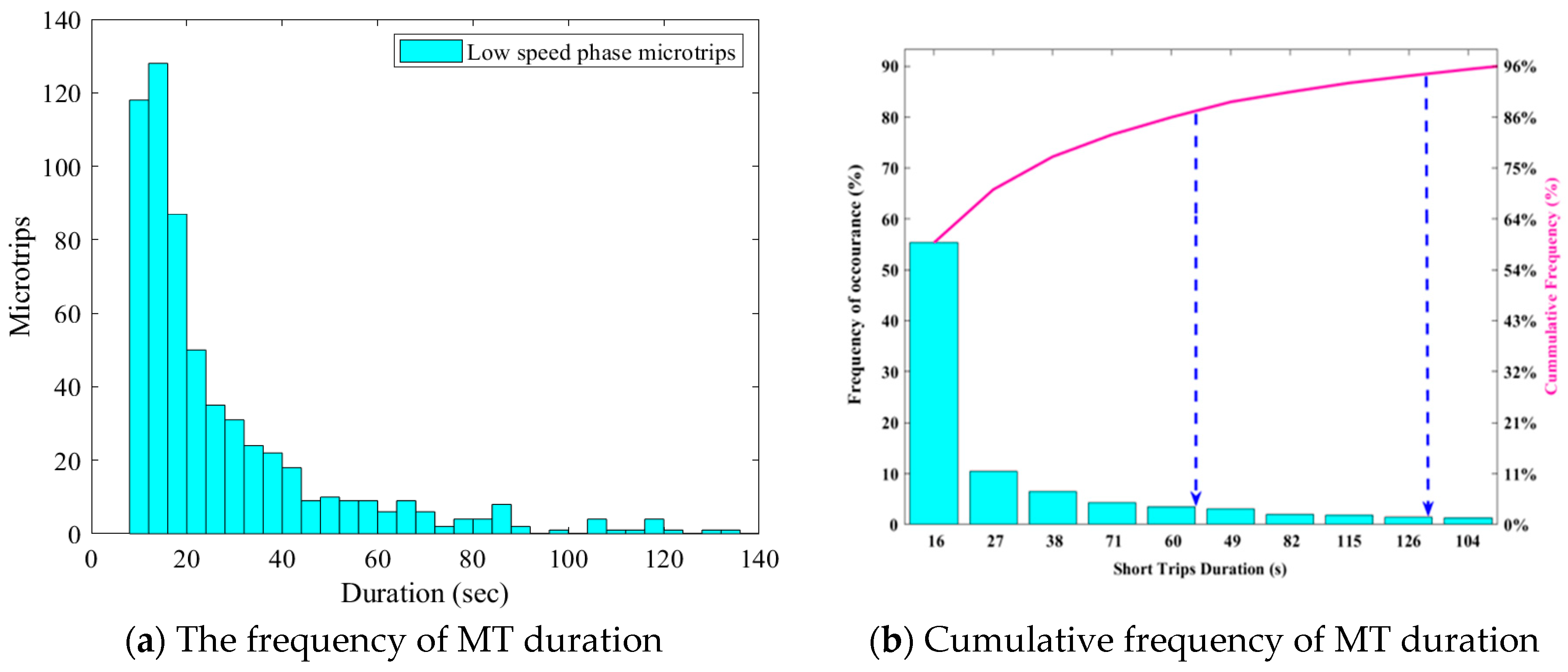
2.4. Trip and Micro Trip Division

A trip cycle here covers the driving profile from the dispatching centre to the destination without a prolonged stop duration. For AA intercity and feeder routes, the segmentation of trips was based on a long stop of more than 1200 s. However, a trip on the ring road and expressways was extracted by matching the Google Maps location with data points. Trip data points established from the criteria set to define kinematic modes, as shown in

Table 3. Criteria set to define kinematic mode trip cycles and micro trips.

Kinematic Mode	Speed (V)	Acceleration (a)	Duration (T)	Distance (D)
Stop mode	V < 1 m/s	>−0.15 m/s2 and <0.15 m/s2	Tidle	0
Acceleration	V > 1 m/s	>0.15 m/s2 and <4.5 m/s2	Tcruz	Dcruz
Cruising	V > 1 m/s	>−0.15 m/s2 and <0.15 m/s2	Taccel	Daccel
Deceleration	V > 1 m/s	<−0.15 m/s2 and >−4.5 m/s2	Tdecel	Ddecel

, were used to remove outliers. Thereafter, the 490 trips found were categorized into three speed phases (low/medium/high) based on a speed threshold of (40/80) [32]. The Addis Ababa and its suburbs route showed the majority of the distance travel at a vehicle speed of 1–40 km/h along 740.68 km (53.3%) and travel in 101,994 s with 69.94% to the whole trips. The lowest distance travel in the medium speed category was 41–80 km/h with only 249.86 km (17.97%) to whole distances travel and taking 26,227 s in the duration of travel (17.99%). The high-speed trips at 81–120 km/h with medium distances of travel at 399.93 km (28.75%) contributed the least, about 17,485 s, which is 12.01% of the whole travel time.

Similarly, filtered and smooth data were classified into micro trip (MT) and stop bins based on criteria set to remove unrealistic values, and there were 4463 MT and 3236 stop data bins. Statistical models were built to obtain an idea of how the different parameters of trip cycles and MTs behaved and what their distribution was.

2.5. Development Methods of Driving Cycle

2.5.1. Random Selection-to-Rebuild with Behaviour Split (RSBS)

A new approach was devised to utilise the suitability of random selection for heterogeneous traffic conditions, such as AASU routes [29], and to characterise the driving behaviour split based on acceleration-related features, focusing on the assessment of their influence on demand power intensity and energy consumption.

The length of the total duration of the candidate cycle for AASU routes was set based on the statistical results of trip cycles, whereas phase durations for each of the three speeds were calculated proportionate to the collected data. The results are presented in

Table 4. Characteristic distribution for short trips and stops of the three-speed phases.

Profile Characteristics	Low	Medium	High
Traffic speed limit (km/h)	30–40	60–80	100–120
Real data proportion (%)	70	18	12
Phase duration (s)	924	238	159
Average short trip duration (s)	64	251	131
Average stop duration (s)	11	5	5
Short trips	10	1	1
Stops	11	2	2

.

Equations (3) and (4) used in the synthesis of WLTC were adapted to determine the optimum number of short trips (ST) for each speed phase. Thus, ten (10) STs were obtained with corresponding eleven (11) stops for the low-speed phase and single but relatively longer trips for the medium and high-speed phases. A separate statistical analysis was performed to assign the first ST and chaining sequence of each. Then, driving behaviour was split based on the position of the average score on a quartile graph obtained from cumulative diagram functions (CDF) of acceleration-related features [33]. The combination of short trips (STs) was made from each mild and aggressive acceleration and braking behaviour.

$${\mathrm{N}}_{\mathrm{ST}}={\mathrm{T}}_{\mathrm{SP}}-{\mathrm{T}}_{\mathrm{AS}}/{\mathrm{T}}_{\mathrm{AST}}-{\mathrm{T}}_{\mathrm{AS}}$$

(3)

$${\mathrm{N}}_{\mathrm{S}}={\mathrm{N}}_{\mathrm{ST}}+1$$

(4)

where N_ST and N_S are the numbers of short trips and stops, and T_SP, T_AST, and T_AS are the durations of speed phase, average short trip, and average stop, respectively. After combining STs, the candidate cycle with the smallest chi-squared values of RPA and RNA were selected from each behaviour. Finally, the combination cycle consisting of each behaviour in proportion to the percentile score distribution was synthesised as a candidate cycle for the AASU driving profile.

2.5.2. K-Means Clustering Method

Here, the k-means clustering approach was implemented to group the samples with data similarity without a given classification category. Initially, the features were scaled to the same range before applying a dimensionality reduction by PCA. Dimensionality reduction was performed by employing principal component analysis (PCA) to avoid crowding and visualise the results more effectively. Then, eigenvectors and eigenvalues of the exposed covariance matrix were calculated, which helped to select the most essential initial features based on the variability being prioritised. The quality and representativeness assessed through the variance were explained using a Pareto graph.

Finally, MTs were grouped by k-means clustering, which calculated the distance between data points to find the closest ones based on their driving features. Prior to clustering, the silhouette coefficient employed and cluster quality were evaluated to find the ideal number of clusters that best fit the data set. A representative number of MTs was selected from each cluster based on their closeness to the cluster centres until a cycle duration of 1320 s cycle was achieved. The duration distribution for each cluster was calculated in proportion to the data count as follows [22]:

$${\mathrm{T}}_{\mathrm{MTC}\left(\mathrm{i}\right)}=({\mathrm{T}}_{\mathrm{C}\left(\mathrm{i}\right)}/{\mathrm{T}}_{\mathrm{DC}}){\mathrm{T}}_{\mathrm{MT}}$$

(5)

where T_MTC(i) is the duration of MT from the ith cluster; T_C(i) is the duration of the ith cluster; T_MT is the total duration of MTs clustered, and T_DC is the total duration of the candidate DC.

3. Results and Discussion

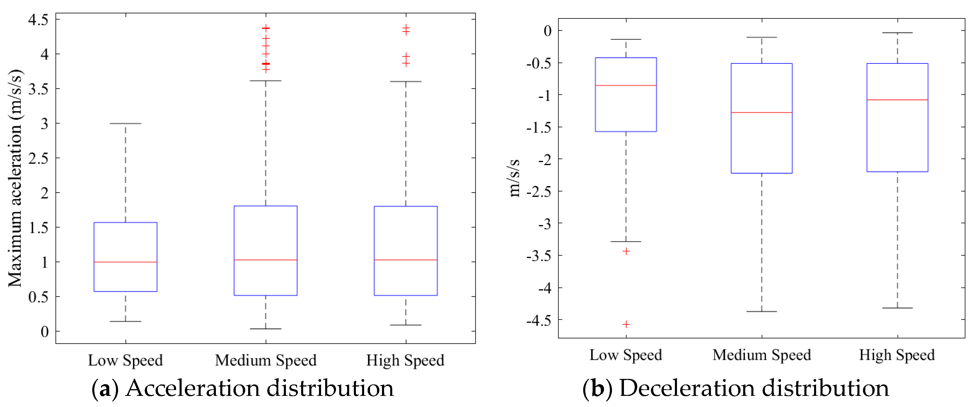
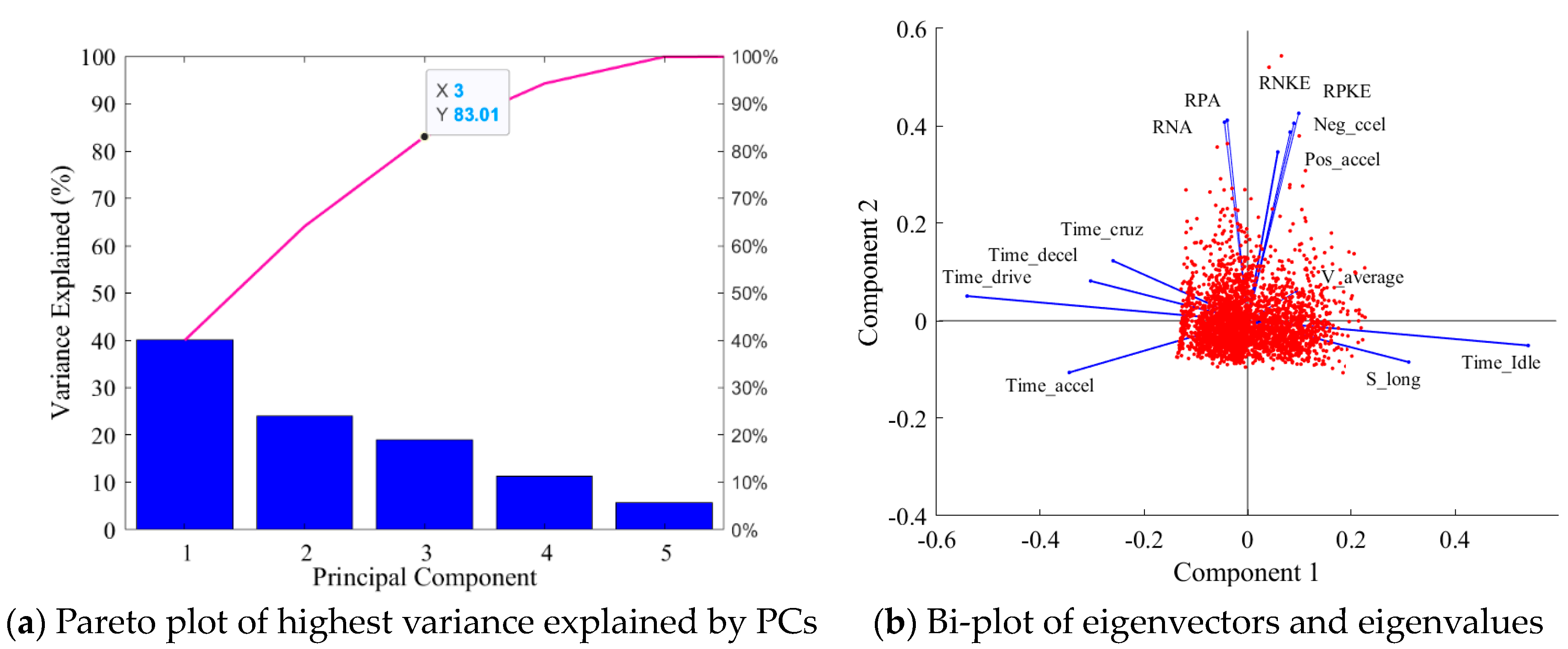
3.1. Results of Statistical Analysis

3.1.1. Real-Data Trip Features

The analysis of trip distances is shown in Figure 4a and recorded an average value of 7.28 km, with the highest frequency in the range of 3–4.5 km. Furthermore, 80% of the trip distances covered less than 9.83 km in CDF. It should be noted that the driven distance of a candidate DC was found to be in a range of 4 km to 15 km but must be near the established CDF value. Regarding trip duration, 25% recorded the highest frequency with a duration of about 750 s (12.5 min). Additionally, the third quartile, as indicated in Figure 4b, was located at 1358 s (22.63 min). Hence, the representative driving cycle should be close to the third quartile, while the duration was adjusted to 1320 s (22 min) to minimise the computational burden.

A significant difference of 46% was noted between the average speeds (w/o stop) and average driving speeds (w/stop) in the low-speed phase compared with 8% in the high-speed phase, as shown in Figure 5a,b. This indicates that the influence of stop time on average vehicle speed was based on the percentage of stop time.

After analysing the CFD of all ten (10) short trips in the low-speed phase, it was found that more than 80% primarily coincided with 64 s (see Figure 6b) heighted in blue (left), and a high frequency (55%) occurred below 20 s (see Figure 6a,b). Hence, the fifth MT, with an average speed of 18 km/h and lasting 64 s, was found to be the best fit with real data and was selected to be the first MT of the low-speed phase. A stop duration between MTs would be steady sampling, and to address the smooth transition, it was decided that the average stop duration of the trip cycle would be 11 s.

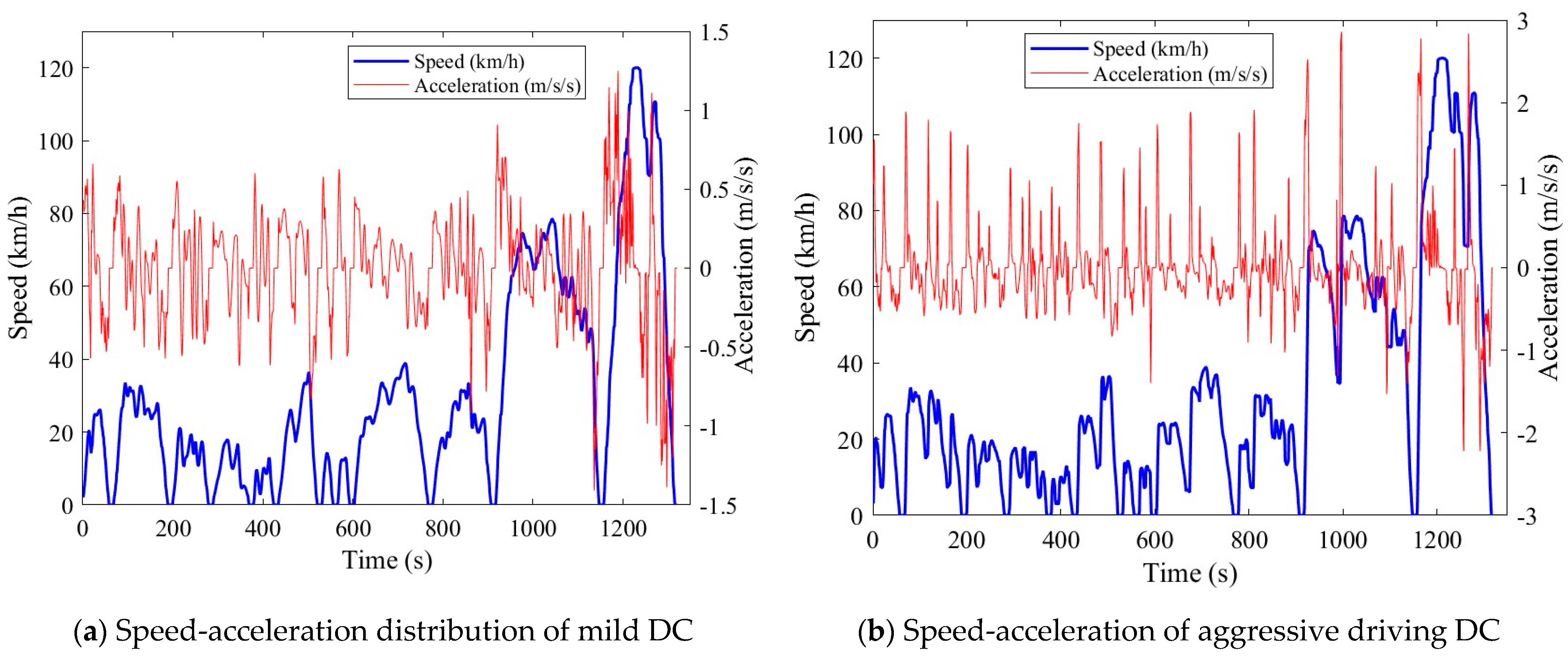
3.1.2. Driving Behaviour Split

Figure 7a,b illustrate the distribution of acceleration-related principal components used for acceleration and braking behaviour splitting.

High-speed phases have a low APA, RPA and time idling but a long distance. A medium APA, high RPA, medium distances, and medium stop time represent the medium-speed phase. Finally, the low-speed phase was found to have a high APA, medium RPA, high stop time and shorter distances.

Different CDFs for positive and negative acceleration features were obtained, as shown in Figure 8a, and driving behaviours were identified by dividing the average position of each MT on the CDF graph of the 0–1st quartile, 1st–3rd quartile, and 3rd–4th quartile.

The driving behaviour with an average a⁺ < 0.5 m/s² was identified as mild and with a⁺ > 2 m/s² as aggressive, with behaviour between the two being average [21]. As shown in Figure 8b, the driving behaviour of the 0–1st quartile scored 40% is mild, the 1st–3rd quartile scored only 40% is average, and the 3rd–4th scored 20% is aggressive. Consequently, only 40% of MTs, rather than half, were considered to be the average drivers identified by moderate braking. Hence, a representative AASU DC must be constructed by incorporating 40% mild, 40% moderate, and 20% aggressive behaviours in both ascending and descending speed profiles.

3.2. Drive Cycle Synthesised by the RSBS Method

The speed-acceleration distribution of the synthesised four cycles (i.e., mild, aggressive driving, aggressive braking, and combined) are presented in Figure 9 and Figure 10.

After behaviour division, the speed difference between mild and aggressive was considerably lower, but a remarkably high variation existed between accelerations in the two behaviours. This variation was lower for the low phase and higher for the high phase. Hence, it could be concluded that as the speed increased, the gap between quartile one and quartile three decreased for both positive and negative accelerations.

For mild cycles (see Figure 9), a low variation in acceleration was found among different driving profiles (−3.75%) with an increase in driving speed, but for aggressive driving, the variation was higher (−22.5%). Although behaviour splitting has a significant influence on urban cycles, a considerable dispersion in acceleration-related features was found in the medium and high-speed segments.

3.3. Drive Cycle Synthesised by the k-Means Method

The Pareto graph in Figure 11a indicates that only five (5) principal components (PCs) achieved the explained variability of 99.8% rather than the twelve (12) PCs implemented. The variance explained by the first, second, and third PCs was 40%, 22.6%, and 19.4%, respectively, and the total variance explained by the employment of the first three PCs was correct since they represented about 82.01% of the data set variability.

The two-dimensional bi-plot presented in Figure 11b shows the contribution and influence of the driving features on the first two PCs. The highest variability was found in speed-related features, distance, and time percentage of the stop because they were the main contributors to the variance explained by the first PC. Acceleration-related features, including APA, ANA, RPA, RNA, PKE, and NKE, mainly influenced the second component. The third component was mainly affected by the stop and time proportion of each kinematic mode.

The three PCs were grouped by k-means into the optimum number of six clusters, as shown in Figure 12b with the higher silhouette value of 0.78, and uniform width obtained when compared with the 0.74 silhouette values and non-uniform widths of five clusters shown in Figure 12a. Short trips were then selected from all the clusters based on their closeness to the cluster centres until a total duration of 1320 s was obtained.

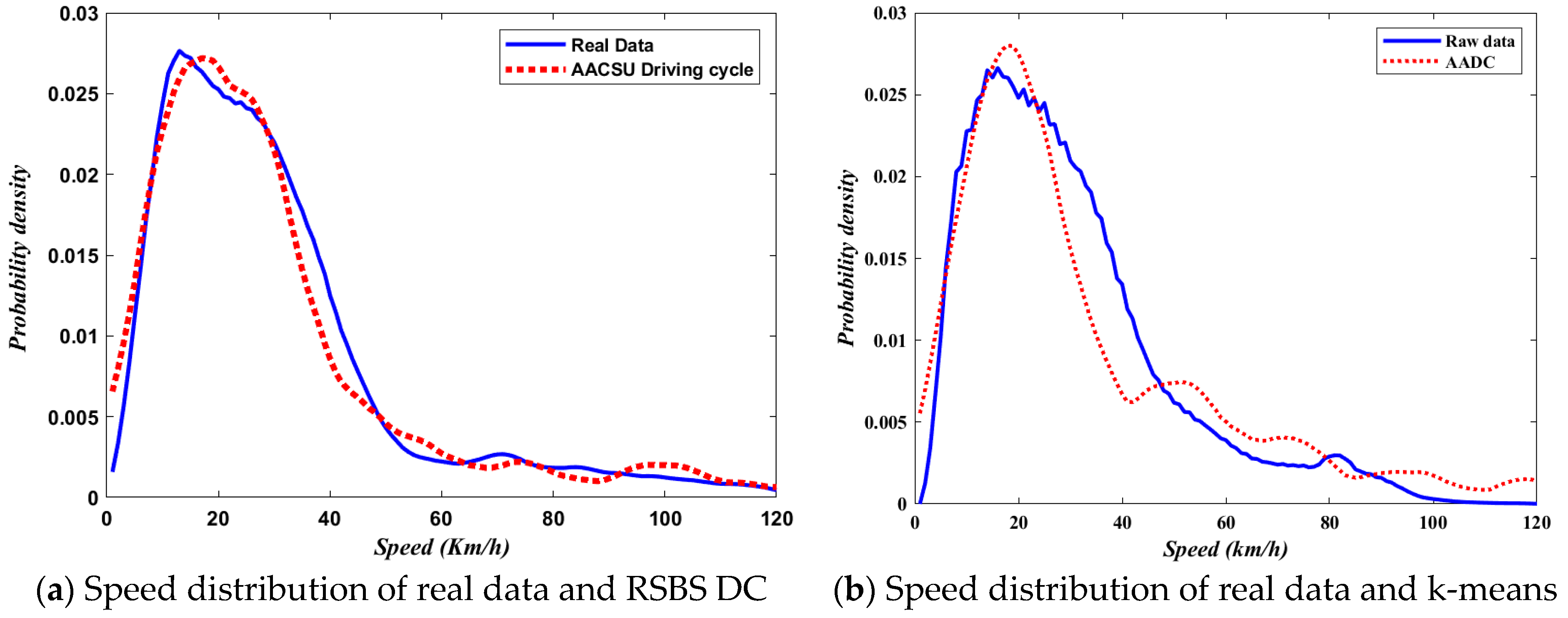
3.4. Characteristic Distribution of Synthesised Drive Cycles and Real Dataset

Relative, mean relative, and root mean square errors of speed and acceleration-related features between candidate DCs and the entire dataset were calculated. The difference between the speed distributions of the real data from DCs by the RSBS and k-means methods were compared and are shown in Figure 13a,b, respectively.

The average difference in RSBS DC from real data was found to be lower (2%) than that of the higher (5%) k-means DC. Other statistical properties are compared in

Table 5. Essential characteristics of RSBS, k-means, WLTC-2 DCs, and real data.

Drive Cycles	Cycle Phase	Duration (s)	V w/o Stops (km/h)	V w/Stops (km/h)	aave (m/s2)	dave (m/s2)	D (km)	RPA (m/s2)	RNA (m/s2)
RSBS	Low	882	19.8	17.6	0.43	−0.46	4.196	0.185	−0.22
	Medium	255	56.1	53.7	0.625	−0.705	2.942	0.5	−0.66
	High	183	81.4	73.9	0.45	−0.61	2.835	0.29	−0.32
k-means	Low	950	18.9	16.7	0.645	−0.645	4.42	0.43	0.40
	Medium	240	40.4	36.4	0.54	−0.705	2.43	0.56	0.65
	High	132	85.4	82.1	0.625	−0.621	3.01	0.72	0.91
Real data	Low	101,994	21.30	14.7	0.44	−0.36	400.	0.34	−0.29
	Medium	26,227	59.75	33.4	0.54	−0.74	249.9	0.63	−0.62
	High	17,485	94.9	78.1	0.39	−0.42	740.7	0.45	−0.36
WLTC−2	Low	589	26.0	51.4	0.92	−1.07	3.132	0.244	0.2112
	Medium	433	44.1	74.7	0.96	−0.99	4.712	0.629	0.2489
	High	455	57.8	85.2	0.85	−1.11	6.820	0.962	0.1994

, which indicates that there was a significant distortion in the statistical distribution of k-means DC from the original data set. However, the relative error between RSBS DC and real data was the lowest, and this was selected as the best representative BEV DC suitable for AASU routes.

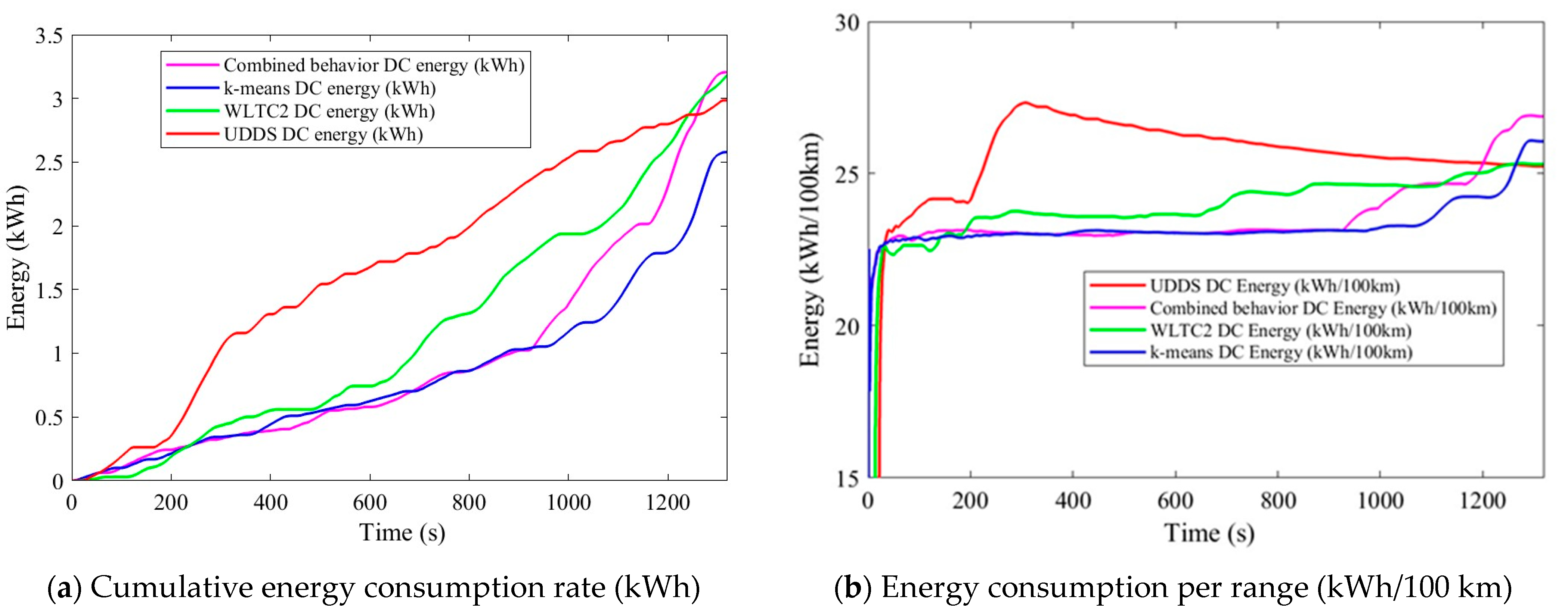
3.5. Comparison of Energy Consumption between Standard and AASU Candidate DCs

In a typical DC, the tractive effort provided by a vehicle’s power/energy source must overcome all road loads, including aerodynamic, rolling, gravitational, and acceleration resistance expressed. Estimation of the on-board energy storage system for BEV was averaged cumulative energy as a function of driving speed over the interval dt:

$${\mathrm{E}}_{\mathrm{Total}}={\displaystyle \underset{0}{\overset{{\mathrm{t}}_{\mathrm{f}}}{\int }}{\mathrm{F}}_{\mathrm{tra}}\mathrm{v}\left(\mathrm{t}\right)\mathrm{dt}}={\displaystyle \underset{0}{\overset{{\mathrm{t}}_{\mathrm{f}}}{\int }}\mathrm{P}\left(\mathrm{t}\right)\mathrm{dt}}$$

(6)

The energy consumed by a 1200 kg mid-size car to negotiate the road load was calculated from the candidate AASU DC among different behaviours for comparison. In Figure 14a, the area under the curve of the aggressive cycle peaked higher at 3.34 kWh at a greater speed compared with the mild cycle’s 3 kWh. Figure 14b shows energy consumption per 100 km. High consumption at high speeds was due to the coupled effect of high speed with high acceleration, which has a considerable correlation with energy consumption.

Figure 15a,b shows a comparison of the effect of braking behaviour division on regenerative potential with coast and panic braking. More braking kinetic energy of 1.65 kWh (21.2%) was wasted by aggressive drivers than the 1.3 kWh wasted by coast drivers. Studies have indicated that the regeneration potential with current advances was only 8% of energy for aggressive drivers and up to 25% for coast drivers [34].

Accordingly, the regenerated energy can extend the range per single charge of BEV by 10.8% and 3.9% for the coast and aggressive drivers, respectively. Hence, splitting behaviour and ignoring braking mode will result in a significant error in net energy consumption estimation and battery size due to the distortion in characteristics of DC synthesised from that of a real driving scenario.

Finally, the averaged RSBS DC was compared with k-means, WLTC-2, and UDDS cycles [2]. The standard cycles were selected based on the equivalence in total duration of WLTC-2 1477 s and UDDS 1400 s, method of construction, and data representativeness. WLTC-2 has the highest maximum acceleration of all cycles, which was thought to be more realistic. The maximum acceleration of UDDS was lower compared with the transient cycles.

The cumulative energy consumption rate and consumption per 100 km by RSBS, k-means, WLTC-2, and UDDS DC were calculated, and the results are shown in Figure 16a,b. Less energy was consumed by RSBS DC than by the WLTC-2 and UDDS cycles at a wide operating range, except at peak velocity.

A significant difference was found with a low overall net consumption per 100 km range of 22.5 kWh compared with 24.25 kWh and 26.34 kWh of WLTC2 and UDDS net consumptions, respectively. Net consumption by RSBS and k-means DC was comparable at low speeds; however, at higher speeds, the k-mean consumed less due to the average low acceleration dispersion.

For the high-speed expressway, part of the RSBS DC, a distinct operating point could be found at 120 km/h, where more energy was consumed and power was demanded (see Figure 17). However, this was because the higher drag force was not related to driving behaviour. Although the consumption was high for high speed, the proportion of the route segment was only 10% compared with 70% for urban and 20% for suburban routes, and the influence on net energy demand per range was insignificant. WLTC-2 demanded high power in the urban DC due to the maximum speed coupled with aggressive acceleration within a short driving range, whereas UDDS required moderate power in a representative rural section, except in an aggressive single trip.

4. Conclusions

In this work, GPS data from highways in Addis Ababa and its suburbs were used to build a minimum energy consumption BEV DC. Two techniques were employed to synthesise the DC, k-means and RSBS.

First, RSBS DC with a minimum error of 2% was chosen after assessing the statistical distribution and representativeness against real data. This was because k-means revealed a considerable distortion with a 5% error. It was discovered through behaviour splitting that drivers who exhibit aggression tend to use more energy due to their frequent panic stops and subsequent accelerations.

When in braking mode, coasters can increase regeneration efficiency by up to 25%. They can extend the range by 18.9%, while aggressive drivers can only achieve 3.9%. Lastly, a comparison of averaged AASU and conventional cycles’ power and energy consumption was made. For the Addis Ababa driving cycle, a notable decrease in energy estimation of 14.57% from UDDS and 8.9% from WLTC-2 was attained. This study’s DC effectively captures Addis Ababa’s and its suburb’s driving profile, and it may be used to calculate the energy consumption of other emerging large cities and vehicle types.

Moreover, this study’s conclusion may be applicable to the grid of power as well as the economic and lifetime analysis of BEVs. It is advised that in the future, driving and road slope profiles be combined in a parallel simulation to help provide a more precise estimate of energy use.

References

1. Pathak, A.; Sethuraman, G.; Krapf, S.; Ongel, A.; Lienkamp, M. Exploration of Optimal Powertrain Design Using Realistic Load Profiles. World Electr. Veh. J. 2019, 10, 56. [Google Scholar] [CrossRef]
2. Lasocki, J. The WLTC vs NEDC: A Case Study on the Impacts of Driving Cycle on Engine Performance and Fuel Consumption. Int. J. Automot. Mech. Eng. 2021, 18, 9071–9081. [Google Scholar] [CrossRef]
3. Khemri, N.; Supina, J.; Syed, F.; Ying, H. Developing a Real-World, Second-by-Second Driving Cycle Database through Public Vehicle Trip Surveys. In SAE Technical Paper Series; SAE International: Warrendale, PA, USA, 2019. [Google Scholar] [CrossRef]
4. Global EV Outlook 2022: Securing Supplies for an Electric Future; International Energy Agency: Paris, France, 2022. [CrossRef]
5. Global EV Outlook 2020: Entering the Decade of Electric Drive; International Energy Agency: Paris, France, 2020.
6. Pakdel Bonab, S.; Kazerooni, A.; Payganeh, G.; Esfahanian, M. Extracting Tehran refuse collection truck driving cycle and estimating the braking energy. Int. J. Automot. Eng. 2020, 10, 3149–3157. [Google Scholar]
7. Lyu, N.; Wang, Y.; Wu, C.; Peng, L.; Thomas, A.F. Using naturalistic driving data to identify driving style based on longitudinal driving operation conditions. J. Intell. Connect. Veh. 2022, 5, 17–35. [Google Scholar] [CrossRef]
8. Bouhsissin, S.; Sael, N.; Benabbou, F. Driver Behavior Classification: A Systematic Literature Review. IEEE Access 2023, 11, 14128–14153. [Google Scholar] [CrossRef]
9. Ghandour, R.; Potams, A.J.; Boulkaibet, I.; Neji, B.; Al Barakeh, Z. Driver behavior classification system analysis using machine learning methods. Appl. Sci. 2021, 11, 10562. [Google Scholar] [CrossRef]
10. Busho, S.W.; Alemayehu, D. Applying 3D-eco routing model to reduce environmental footprint of road transports in Addis Ababa City. Environ. Syst. Res. 2020, 9, 17. [Google Scholar] [CrossRef]
11. Zhao, M.; Gao, H.; Han, Q.; Ge, J.; Wang, W.; Qu, J.; Vanajakshi, L. Development of a Driving Cycle for Fuzhou Using K-Means and AMPSO. J. Adv. Transp. 2021, 2021, 5430137. [Google Scholar] [CrossRef]
12. Thomas, D.B. Real World Driving Emissions from Hybrid Electric Vehicles and the Impact of Biofuels. Ph.D. Thesis, University of Leeds, Leeds, UK, 2020. [Google Scholar]
13. Huzayyin, O.A.; Salem, H.; Hassan, M.A. A representative urban driving cycle for passenger vehicles to estimate fuel consumption and emission rates under real-world driving conditions. Urban Clim. 2021, 36, 100810. [Google Scholar] [CrossRef]
14. Hayes, J.G.; Goodarzi, G.A.J.I.A.; Magazine, E.S. Book review: Electric powertrain: Energy systems, power electronics and drives for hybrid, electric and fuel cell vehicles. IEEE Aerosp. Electron. Syst. Mag. 2019, 34, 46–47. [Google Scholar] [CrossRef]
15. Rodrigues, C.D.P. Design of a High-Speed Transmission for an Electric Vehicle. Master’s Thesis, University of Porto, Porto, Portugal, 2018. [Google Scholar]
16. Jacobson, B. Vehicle Dynamics Compendium for Course MMF062, 2016th ed.; Chalmers University of Technology: Gothenburg, Sweden, 2016. [Google Scholar]
17. Yu, Y.; Jiang, J.; Wang, P.; Li, J. A-EMCS for PHEV based on real-time driving cycle prediction and personalized travel characteristics. Math. Biosci. Eng. MBE 2020, 17, 6310–6341. [Google Scholar] [CrossRef] [PubMed]
18. Sayed, K.; Kassem, A.; Saleeb, H.; Alghamdi, A.S.; Abo-Khalil, A.G. Energy-Saving of Battery Electric Vehicle Powertrain and Efficiency Improvement during Different Standard Driving Cycles. Sustainability 2020, 12, 10466. [Google Scholar] [CrossRef]
19. Wang, S.; Wang, J.; Song, L.; Niu, Z.; Hu, X. Design of two-regional flexible-route bus systems considering interregional demands. J. Adv. Transp. 2022, 2022, 9372011. [Google Scholar] [CrossRef]
20. Peng, J.; Jiang, J.; Ding, F.; Tan, H. Development of Driving Cycle Construction for Hybrid Electric Bus: A Case Study in Zhengzhou, China. Sustainability 2020, 12, 7188. [Google Scholar] [CrossRef]
21. Zhao, D.; Zhong, Y.; Fu, Z.; Hou, J.; Zhao, M.; Galante, F. A Review for the Driving Behavior Recognition Methods Based on Vehicle Multisensor Information. J. Adv. Transp. 2022, 2022, 7287511. [Google Scholar] [CrossRef]
22. Chandrashekar, C.; Agrawal, P.; Chatterjee, P.; Pawar, D.S. Development of E-rickshaw driving cycle (ERDC) based on micro-trip segments using random selection and K-means clustering techniques. IATSS Res. 2021, 45, 551–560. [Google Scholar] [CrossRef]
23. Han, B.; Wu, Z.; Gu, C.; Ji, K.; Xu, J. Developing a Regional Drive Cycle Using GPS-Based Trajectory Data from Rideshare Passenger Cars: A Case of Chengdu, China. Sustainability 2021, 13, 2114. [Google Scholar] [CrossRef]
24. Khadhir, A.; Bhaskar, A.; Vanajakshi, L.; Haque, M.M. Development of a theoretical delay model for heterogeneous and less lane-disciplined traffic conditions. J. Adv. Transp. 2022, 2022, 3260945. [Google Scholar] [CrossRef]
25. Chen, A.H.; Liang, Y.-C.; Chang, W.-J.; Siauw, H.-Y.; Minanda, V. RFM model and K-means clustering analysis of transit traveller profiles: A case study. J. Adv. Transp. 2022, 2022, 1108105. [Google Scholar] [CrossRef]
26. Gebisa, A.; Gebresenbet, G.; Gopal, R.; Nallamothu, R.B. A Neural Network and Principal Component Analysis Approach to Develop a Real-Time Driving Cycle in an Urban Environment: The Case of Addis Ababa, Ethiopia. Sustainability 2022, 14, 13772. [Google Scholar] [CrossRef]
27. Liu, T.; Tan, W.; Tang, X.; Zhang, J.; Xing, Y.; Cao, D. Driving conditions-driven energy management strategies for hybrid electric vehicles: A review. Renew. Sustain. Energy Rev. 2021, 151, 111521. [Google Scholar] [CrossRef]
28. Singh, M.K.; Pathivada, B.K.; Rao, K.R.; Perumal, V. Driver behaviour modelling of vehicles at signalized intersection with heterogeneous traffic. IATSS Res. 2022, 46, 236–246. [Google Scholar] [CrossRef]
29. Kabalan, B. Systematic Methodology for Generation and Design of Hybrid Vehicle Powertrains. Ph.D. Thesis, Université de Lyon, Lyon, France, 2020. [Google Scholar]
30. Zhou, Y.; Ravey, A.; Péra, M.-C. A survey on driving prediction techniques for predictive energy management of plug-in hybrid electric vehicles. J. Power Sources 2019, 412, 480–495. [Google Scholar] [CrossRef]
31. Rashed, G.I.; Li, X.; Pang, Z.; Zhao, H.; Kheshti, M. Research on Construction Method of Urban Driving Cycle of Pure Electric Vehicle. E3S Web Conf. 2021, 252, 02064. [Google Scholar] [CrossRef]
32. Nagaraj, S. Algorithm to Generate Synthetic Driving Cycle Using Real Driving Data. Master’s Thesis, Chalmers University of Technology, Göteborg, Sweden, 2021. [Google Scholar]
33. Yuan, T.; Liu, R.; Zhao, X.; Yu, Q.; Zhu, X.; Wang, S. Analysis of normal stopping behavior of drivers at urban intersections in China. J. Adv. Transp. 2022, 2022, 7588589. [Google Scholar] [CrossRef]
34. Gao, Z.; LaClair, T.; Ou, S.; Huff, S.; Wu, G.; Hao, P.; Boriboonsomsin, K.; Barth, M. Evaluation of electric vehicle component performance over eco-driving cycles. Energy 2019, 172, 823–839. [Google Scholar] [CrossRef]
Figure 1. Road network of the study area of AA and suburbs.
Wevj 14 00302 g001
Figure 2. Step-by-step flow chart of data filtration and driving cycle development.
Wevj 14 00302 g002
Figure 3. Speed-acceleration distribution of the unified and filtered dataset.
Wevj 14 00302 g003
Figure 4. Distance and duration distributions of real-time trip cycles.
Wevj 14 00302 g004
Figure 5. Comparison of driving speeds.
Wevj 14 00302 g005
Figure 6. The distribution of low-speed short trip duration.
Wevj 14 00302 g006
Figure 7. Acceleration and deceleration distribution of low, medium, and high-speed trip cycles.
Wevj 14 00302 g007
Figure 8. Cumulative distribution function and its quartile score of acceleration.
Wevj 14 00302 g008
Figure 9. Speed-acceleration distributions of ACSU representative DC by the RSBS method.
Wevj 14 00302 g009
Figure 10. Speed-acceleration of the DC by the RSBS method for aggressive and combined behaviours.
Wevj 14 00302 g010
Figure 11. Contribution and influence of driving features on PCs and their variance explained.
Wevj 14 00302 g011
Figure 12. Score of silhouette value and distribution of width for five and six clusters.
Wevj 14 00302 g012
Figure 13. Comparison of speed distribution between real data and DCs of RSBS and k-means.
Wevj 14 00302 g013
Figure 14. Comparison of energy consumption for different driving behaviours of AASU.
Wevj 14 00302 g014
Figure 15. Regenerative potential of mild and aggressive driving behaviours representative of AASU DCs.
Wevj 14 00302 g015
Figure 16. Comparison of energy consumption between WLTC-2, UDDS, and AASU candidate DCs by RSBS and k-means.
Wevj 14 00302 g016
Figure 17. Comparison of power consumption between WLTC-2, UDDS, and AASU candidate DCs by RSBS and k-means methods.
Wevj 14 00302 g017