Research on Vegetation Cover Changes in Arid and Semi-Arid Region Based on a Spatio-Temporal Fusion Model

Abstract

Vegetation dynamics in arid and semi-arid regions have an important impact on carbon cycle, water cycle, and energy exchange at local, regional, and global scales. Therefore, it is of great significance for scientists to grasp the changes of vegetation cover in arid and semi-arid regions timely and accurately. Based on this, the applicability of ESTARFM model in the complex terrain area of arid and semi-arid Xinjiang was explored using Landsat and MODIS data fusion, and the overall change characteristics of vegetation cover (FVC) and the distribution and change patterns of different terrains in the study area in the past 15 years were analyzed by combining the dimidiate pixel model, unary linear regression and digital elevation model. The results show that: (1) the NDVI data fused by ESTARFM Model has high consistency with the real NDVI data, and it can be used for subsequent FVC estimation. (2) From 2006 to 2020, the inter FVC was at a high level as a whole, and the average annual FVC showed a weak increasing trend in fluctuation; there are obvious differences in spatial distribution, which is characterized by high distribution in the north and low in the south. (3) The improved area of vegetation cover in the study area is greater than the degraded area, accounting for 52.3% and 47.7% respectively; (4) In the elevation range of 2000 to 3500 m, the FVC showed a slight degradation trend on 25° to 45° slopes and south and southeast slopes, and the rest showed a slight improvement trend. ESTARFM-based model enables monitoring of vegetation cover changes in complex terrain areas of the arid and semi-arid regions in Xinjiang over a long time series. The overall FVC level in the study area is high, and there both are serious degradation and improvement phenomena.

1. Introduction

Vegetation is an important component of terrestrial ecosystems and plays an irreplaceable role in global material and energy cycling, regulating carbon balance, and maintaining climate stability [1,2,3,4], as well as an “indicator” of global ecosystem changes [5,6]. The monitoring of dynamic changes of vegetation has long been important and studied by many scholars at home and abroad [7,8,9,10]. Vegetation cover (FVC) is the percentage of the vertical projected area of the above-ground part of vegetation (including leaves, stems, and branches) on the ground to the total area of the statistical area [11], which is a comprehensive quantitative indicator describing the growth of vegetation on the ground and an important indicator of the regional ecosystem environment [12,13].

Two methods are mainly used to study FVC: ground survey method and remote sensing monitoring method [14,15]. The traditional ground survey method has problems such as large workload, high labor intensity, and difficulty in achieving monitoring of long time series. With the continuous development of remote sensing technology, the use of remote sensing technology to monitor vegetation changes has become a feasible means and has been widely used [16,17]. Some scholars have estimated and analyzed the FVC change trends in Tianshan or North Tianshan for the past 16 years based on 3–5 Landsat TM images, respectively [18,19,20]. Some scholars have also studied the changes in vegetation cover or grassland cover and their influencing factors in Xinjiang and even in a larger region based on MODIS data [21,22]. Another group of scholars studied the vegetation growth trends in China (Northwest) based on the GIMMS dataset and analyzed to expose the influencing factors [23,24,25].

From the above studies, it can be found that MODIS and GIMMS data are time-sensitive and can better express the time-series changes of FVC, especially for the monitoring of abrupt change years; by contrast, Landsat data have higher spatial resolution and can achieve finer monitoring of vegetation change information, but it is difficult to find abrupt change information in time-series change monitoring due to the limitations of data re-simulation period and cloud volume [18,21]. Gao et al. [26] first proposed the spatial and temporal adaptive reflection fusion model (STARFM) in 2006 to achieve the fusion of Landsat images and MODIS images. This model can accurately predict reflectance values with high spatial and temporal resolution. However, the STARFM model also has limitations, and the method does not fuse well in areas with high heterogeneity. In view of this limitation, Zhu et al. [27] proposed the enhanced spatio-temporal adaptive reflection fusion model (ESTARFM) in 2010. This model improved the con-version coefficient based on the STARFM model to improve the accuracy of image fusion in heterogeneous regions. It was shown that the model has higher fusion accuracy in complex surface mountainous areas.

Xinjiang is a typical arid and semi-arid region with an extremely fragile internal ecological environment, and the West Tianshan forest region within its territory is one of the areas rich in vegetation resources and plays the role of an ecological barrier in western China [28]. The topography in this region is complex and undulating, and each topographic factor has a complex and integrated influence on the vegetation growth environment, so it is important to carry out vegetation change research with high spatial resolution for ecological environmental protection in complex topographic areas. On the other hand, the ecological environment in this area is complex and extremely sensitive to climate change and human activities, so monitoring vegetation change in time series can help to discover the year of sudden vegetation change, and then analyze the change factors to achieve ecological environmental protection more accurately. However, there is no research on the analysis of vegetation change in this region based on long time series remote sensing data with high spatial resolution. In this paper, based on Landsat data and MODIS data, the ESTARFM model was used to fuse the high spatial resolution time series normalized vegetation index (NDVI) data of each growing season in the study area from 2006 to 2020, and the image dichotomy model was used to estimate the FVC. The distribution and change characteristics of FVC under different topographic factors were revealed by combining with digital elevation model (DEM), in order to provide reference for ecological environment improvement in semi-arid areas of Xinjiang.

2. Materials and Methods

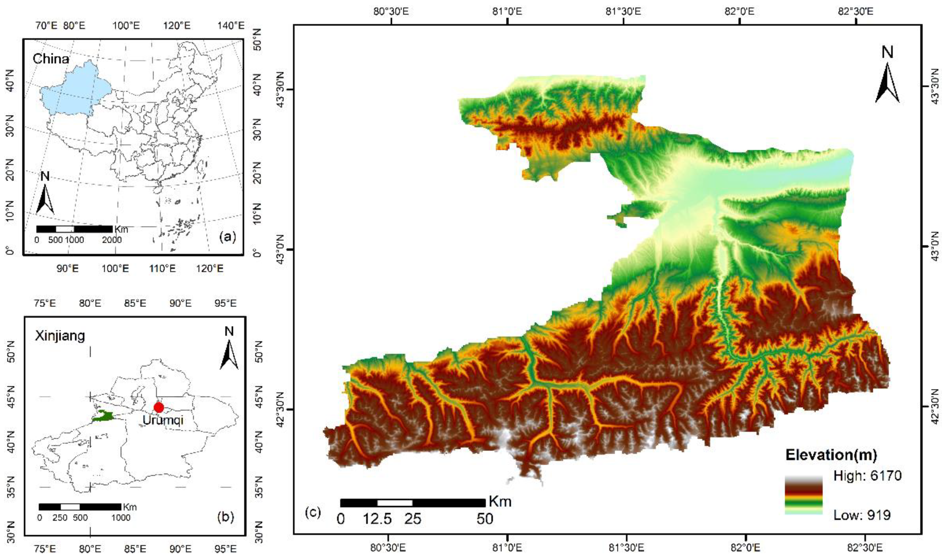
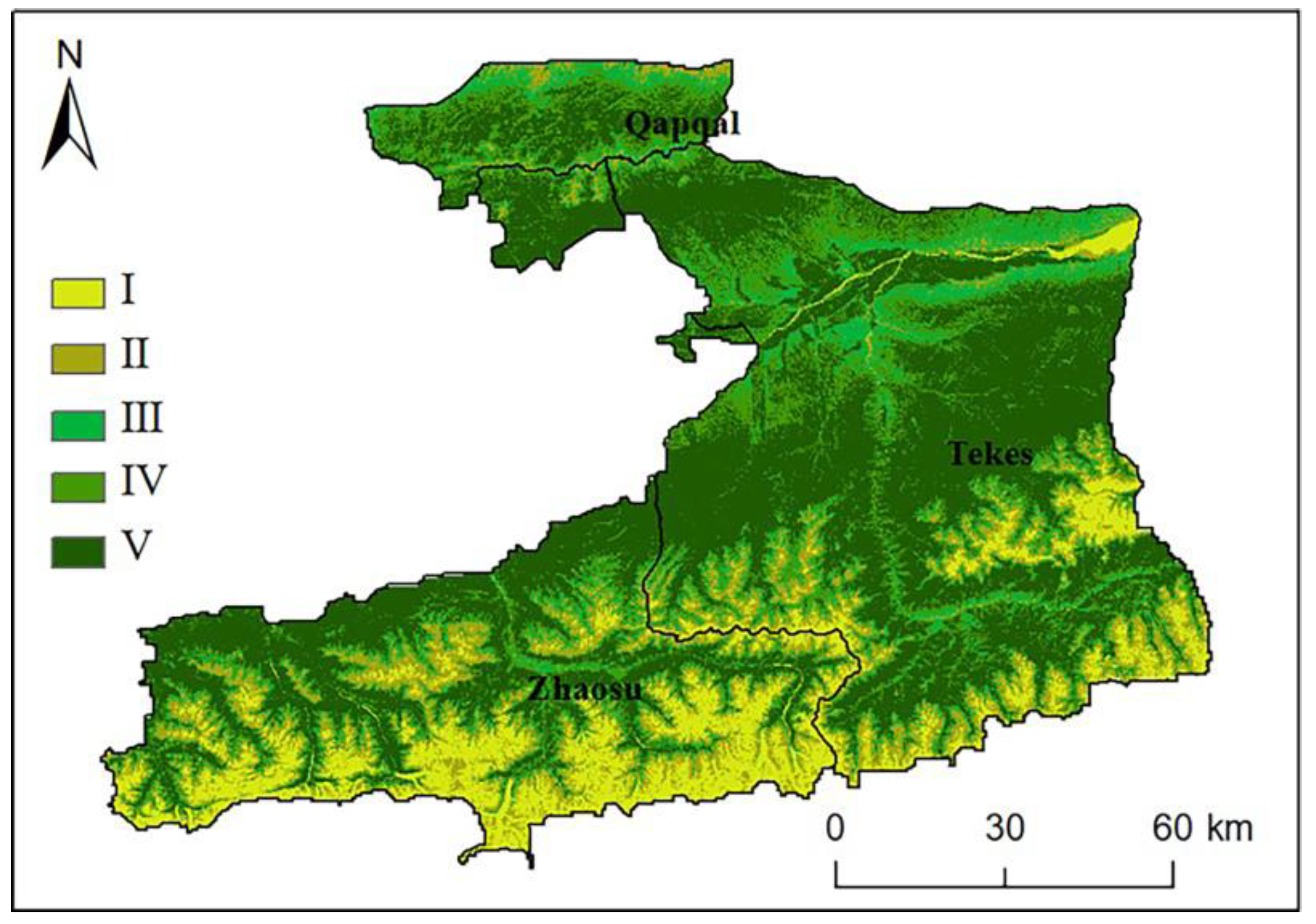
2.1. Study Area

Tekes Forest Farm, Qapqal Forest Farm and Zhaosu Forest Farm of the State-owned Forest Administration Bureau in the Western Tianshan Mountains of Xinjiang Uygur Autonomous Region are selected as the study areas in this study. They are mainly located in Ili Region, with a geographical location of 42°15′26″–43°33′38″ N, 80°12′19″–82°37′52″ E, with a total area of about 14,656 km² (Figure 1). The overall terrain is high in the north and south and low in the middle with an altitude of about 919~6170 m, an average sea wave of 2725 m, and undulating terrain. The study area is deeply inland and belongs to a temperate continental semi-arid climate. The annual and daily temperature range is large. The average annual temperature in the mountain area is 2.8 °C, and the average annual temperature in the river valley is 5.3 °C; on the other hand, it has more precipitation than surrounding areas due to its location in the mid latitude westerly belt and the influence of mountains as well as water vapor from the Atlantic Ocean. It is the precipitation center in the arid region of Central Asia, with an annual precipitation of 550~700 mm. The soil vertical zones in the study area are relatively complete, including mountain chestnut soil, mountain chernozem, mountain leaching taupe forest soil, mountain common taupe forest soil, and mountain grass taupe forest soil.

2.2. Data Source and Pre-Processing

To avoid errors in monitoring results caused by seasonal changes in cloud cover and vegetation, the selected remote sensing data are Landsat series data and MOD09A1 data from July-August, the peak vegetation growth season each year. The cloud amount is less than 10% and the data source is the United States Geological Survey (USGS) (https://earthexplorer.usgs.gov/, accessed on 28 May 2021). The interval between MOD09A1 data collection time and Landsat data is not more than 4 days. Please refer to Appendix A 

Table A1. Information about Landsat remote sensing data used in this study.

Date Acquired	Sensor	Spatial Resolution	Path/Row	Landsat Scene Identifier
14 August 2006	TM	30 m	146/030, 146/031	LT51460302006226IKR00, LT51460312006226IKR00
17 August 2007	TM	30 m	146/030, 146/031	LT51460302007229IKR00, LT51460312007229IKR00
3 August 2008	TM	30 m	146/030, 146/031	LT51460302008216KHC01, LT51460312008216KHC01
11 July 2011	TM	30 m	146/030, 146/031	LT51460302011192IKR02, LT51460312011192IKR02
22 August 2012	ETM+	30 m	146/030, 146/031	LE71460302012235PFS00, LE71460312012235PFS00
1 August 2013	OLI	30 m	146/030, 146/031	LC81460302013213LGN02, LC81460312013213LGN02
19 July 2014	OLI	30 m	146/030, 146/031	LC81460302014200LGN01, LC81460312014200LGN01
9 August 2016	OLI	30 m	146/030, 146/031	LC81460302016222LGN01, LC81460312016222LGN01
15 August 2018	OLI	30 m	146/030, 146/031	LC81460302018227LGN00, LC81460312018227LGN00
17 July 2019	OLI	30 m	146/030, 146/031	LC81460302019198LGN00, LC81460312019198LGN00
4 August 2020	OLI	30 m	146/030, 146/031	LC81460302020217LGN00, LC81460312020217LGN00

and

Table A2. Information about the MODIS remote sensing data used in this study.

Date Acquired	Product Type	Spatial Resolution	Horizontal/Vertical Tile Number	Entity Identifier
13 August 2006	MOD09A1	500 m	h23v04	MOD09A1.A2006225.h23v04.006
13 August 2007	MOD09A1	500 m	h23v04	MOD09A1.A2007225.h23v04.006
4 August 2008	MOD09A1	500 m	h23v04	MOD09A1.A2008217.h23v04.006
12 July 2011	MOD09A1	500 m	h23v04	MOD09A1.A2011193.h23v04.006
20 August 2012	MOD09A1	500 m	h23v04	MOD09A1.A2012233.h23v04.006
28 July 2013	MOD09A1	500 m	h23v04	MOD09A1.A2013209.h23v04.006
20 July 2014	MOD09A1	500 m	h23v04	MOD09A1.A2014201.h23v04.006
12 August 2016	MOD09A1	500 m	h23v04	MOD09A1.A2016225.h23v04.006
13 August 2018	MOD09A1	500 m	h23v04	MOD09A1.A2018225.h23v04.006
20 July 2019	MOD09A1	500 m	h23v04	MOD09A1.A2019201.h23v04.006
4 August 2020	MOD09A1	500 m	h23v04	MOD09A1.A2020217.h23v04.006

for specific information of remote sensing data. There are 11 years of directly available Landsat data from 2006 to 2020, and the years to be predicted are shown in

Table 1. Study Area Demand Forecast Data 2006–2020.

Year	Forecast Date	Year	Forecast Date
2007 (Experiment)	08.13	2015	08.13
2009	08.13	2017	08.13
2010	08.13	2019 (Experiment)	08.13

, where the predicted data for 2007 and 2019 are correlated with Landsat TM data for 2007 and Landsat OLI data for 2019 to verify the feasibility of the ESTARFM algorithm. The auxiliary data include the administrative map of the Tianxi Bureau and the DEM data with a spatial resolution of 30 m from the USGS.

The Landsat data are radiometric calibrated, atmospheric corrected, mosaic, and cropped by ENVI software to obtain the image map of the study area. MRT (MODIS Reconstruction Tool) Tool is used for splicing MOD09A1 data, converting the projection into the same projection as that of Landsat. The infrared band and near-infrared band were selected as the bands, and the nearest neighbor sampling method was used for re-projecting the data to the same 30 m spatial resolution as Landsat data, and was outputted in GEOTIFF format. ENVI software is used for cutting the processed MOD09A1 data to ensure that the boundary range and pixel size are consistent with the Landsat data after cutting. Pre-processing was carried out, such as splicing, re-projection and clipping of DEM data, and altitude, slope and slope direction were extracted using ArcGIS software and spatial analysis tools.

2.3. Research Methods

2.3.1. ESTARFM Spatiotemporal Fusion MODEL

ESTARFM Model requires two pairs of high-resolution and low-resolution images acquired in the same period, and a set of low-resolution images used for predicting dates [27]. The Model sets a sliding window of a certain size around the predicted pixel, and convolutes the pixels in the window with the weight function to obtain the predicted value of the central pixel. The sliding window moves one by one on the whole image to obtain the predicted image. The calculation Formula is as follows:

$$L\left(x_{\frac{w}{2}},y_{\frac{w}{2}},t_p,B\right)=L\left(x_{\frac{w}{2}},y_{\frac{w}{2}},t_0,B\right)+{\sum }_{i=1}^N{W}_i\times V_i\times \left(M\left(x_i,y_i,t_p,B\right)-M\left(x_i,y_i,t_0,B\right)\right)$$

(1)

$${\beta }_t=\frac{\frac{1}{\left|{\sum }_{j=1}^w{\sum }_{i=1}^{w}M\left(x_i,y_j,t_{\beta },B\right)-{\sum }_{j=1}^w{\sum }_{i=1}^{w}M\left(x_i,y_j,t_p,B\right)\right|}}{{\sum }_{t=b,e}\left(\frac{1}{\left|{\sum }_{j=1}^w{\sum }_{i=1}^{w}M\left(x_i,y_j,t_{\beta },B\right)-{\sum }_{j=1}^w{\sum }_{i=1}^{w}M\left(x_i,y_j,t_p,B\right)\right|}\right)},\left(t=b,e\right)$$

(2)

$$L(x_{\frac{w}{2}},y_{\frac{w}{2}},t_p,B)={\beta }_b\times L(x_{\frac{w}{2}},y_{\frac{w}{2}},t_b,B)+{\beta }_e\times L(x_{\frac{w}{2}},y_{\frac{w}{2}},t_e,B)$$

(3)

where, L represents Landsat data; M represents MODIS data; w is the size of the sliding window; (x_w/2,y_w/2) represents the center position of the pixel to be measured; B represents the band of the image; L(x_w/2,y_w/2,t_p,B) is the predicted high-resolution pixel value at time t_p; L(x_w/2,y_w/2,t₀,B) is the high-resolution pixel value at t₀; N is the number of similar pixels including predicted pixels; (x_i,y_i) is the position of the ith similar pixel; W_i is the weight of the ith similar pixel jointly determined by the distance of space, time and spectrum; V_i is the conversion coefficient of similar pixels.

In Equation (1), the following aspects need to be noted:

(a) Determining the window size. The window size w is set to 25 according to the recommended parameters used by Zhu [27].

(b) Searching for similar image elements, which are obtained based on the spectral similarity of Landsat NDVI data to the central image element (x_w/2,y_w/2) using a sliding window w search.

(c) Calculation of weights. To calculate the weights, we first calculate the correlation coefficient Ri between Landsat NDVI and MODIS NDVI data, and then find the geographic distance di between the similar image element and the central image element, and finally find the weight Wi of the similar image element to the central image element based on the correlation coefficient and geographic distance.

$$R_i=\frac{E\left[\left(L_i-E\left(L_i\right)\right)\left(M_i-E\left(M_i\right)\right)\right]}{\sqrt{D\left(L_i\right)}\times \sqrt{D\left(M_i\right)}}$$

(4)

$$L_i=\left\{L\left(x_i,y_i,T_b,B_1\right),···L\left(x_i,y_i,T_b,B_n\right),L\left(x_i,y_i,T_e,B_1\right),\dots ,L\left(x_i,y_i,T_e,B_n\right)\right\}$$

(5)

$$M_i=\left\{M\left(x_i,y_i,T_b,B_1\right),···M\left(x_i,y_i,T_b,B_n\right),M\left(x_i,y_i,T_e,B_1\right),\dots ,M\left(x_i,y_i,T_e,B_n\right)\right\}$$

(6)

In Equations (4)–(6), the correlation coefficient is found for each similar image element, i represents the ith similar image element. L_i/M_i is the ith similar image element data set of Landsat/MODIS image, respectively. b is the number of bands, e is the mean value, and d is the variance. The value of correlation coefficient R is in the range of (−1, 1), and the value of R is positively correlated with the spectral similarity.

$$d_i=1+\frac{\sqrt{{\left(x_{w/2}-x_i\right)}^2+{\left(y_{w/2}-y_i\right)}^2}}{\frac{w}{2}}$$

(7)

where d_i is the geographic distance between the similar image element and the central image element, and the larger d_i is, the farther the geographic distance is.

Based on the above, the weighting formula is as follows.

$$D_i=(1-R_i)\times d_i$$

(8)

$$w_i=\frac{1/D_i}{{\sum }_{i=1}^N\left(1/D_i\right)}$$

(9)

where the range of the weight w_i values is (0, 1) and the sum of the weights of all similar image elements is 1.0.

(d) Calculate the conversion coefficients.

$$V_i=\frac{L_{ib}-L_{ie}}{M_{ib}-M_{ie}}$$

(10)

where L_ia, L_ie, M_ia, and M_ie are the image element values of Landsat and MODIS data corresponding to different periods (T_b and T_e) respectively, i.e., different image elements correspond to different conversion factors.

Through Formula (1), MODIS data of two different periods (t_b and t_e) are selected for calculating the high-resolution image reflectance of the prediction date T_p, which is recorded as L_b (x_w/2,y_w/2,t_p,B) and L_e (x_w/2,y_w/2,t_p,B). Combining the two prediction results, the predicted central pixel reflectance is more accurate. The weight is calculated as Formula (2) with higher weight closer to the prediction period as the criterion. The high-resolution reflectance data of the final prediction time is calculated by Formula (3) [27].

Based on different fusion sequences, the ESTARFM model has two schemes. Fusion then Index (BI) and Index then Fusion (IB). BI first simulates the reflectance of the predicted date image and then calculates the vegetation index based on the pre-predicted reflectance; IB calculates the vegetation index first and then uses these vegetation index data to simulate the vegetation index of the predicted date. According to Jarihani et al. [29], the IB scheme has lower computational cost and less error compared with the BI scheme. On this basis, in this paper, continuous normalized vegetation index data with high spatial resolution are obtained by fusion of IB schemes.

2.3.2. FVC Estimation

Methods for measuring FVC based on remote sensing data chiefly include the regression model method, vegetation index method, and pixel decomposition model [30]. Among them, the pixel dichotomous model in the pixel decomposition model is commonly used. Its principle is that, assuming that the surface corresponding to each pixel only contains two components, vegetation and bare land, the proportion of vegetation in the pixel is the FVC of the pixel. The calculation formula is [31]:

$$FVC=\frac{S-S_{\mathit{soil}}}{S_{veg}-S_{soil}}$$

(11)

where FVC denotes the vegetation cover, S is the remote sensing information reflected by each image element, S_soil is the remote sensing information reflected by pure bare ground cover image element, and S_veg is the remote sensing information reflected by pure vegetation cover image element. Rundquist [32] showed that NDVI has a good correlation with FVC, which is in line with the conditions of pixel binary model. Li [33] established a FVC estimation model based on NDVI, and the calculation formula is:

$$FVC=\frac{NDVI-NDV{I}_{\mathit{soil}}}{NDV{I}_{veg}-NDV{I}_{soil}}$$

(12)

where NDVI_soil is the NDVI value of pure bare ground cover image elements and NDVI_veg is the NDVI value of pure vegetation cover image elements. Due to the influence of meteorological elements, vegetation types, and spatial and temporal differences, NDVI_soil and NDVI_veg will vary in different images. Based on the experience of previous studies [33], combined with the histogram of NDVI frequency distribution in this experiment, the cumulative frequency values of 5% and 95% were selected to represent different NDVI_soil and NDVI_veg in different years, respectively, and the FVC was classified into five levels with reference to the Soil Erosion Classification and Grading Standard and related studies [34]. The very low FVC is <10%, the low FVC is 10%–30%, the medium-low FVC is 30%–50%, the medium-high FVC is 50%–70%, and the high FVC is >70%.

2.3.3. Accuracy Verification

In this paper, we use the subimage comparison method based on the comparison of high-resolution images of the same period to validate the vegetation cover estimated based on Landsat data in the Western Tian Shan [35,36]. The pretreated 18 August 2019 Gaofen-1 Image (2 m) and 11 August 2019 Landsat Image were randomly selected for verification, 100 sample points on the Landsat Image were evenly selected and mapped to the Gaofen-1 Image, and the 225 Gaofen-1 pixels corresponding to each sample point were directly manually digitized to calculate the actual FVC. Then, the FVC estimated by the pixel binary model was compared and analyzed, and the model accuracy was judged by the Root Mean Square Error (RMSE). The RMSE Calculation Formula is:

$$RMSE={\left[{\displaystyle \sum }_{i=1}^n\frac{{\left(X_i-Y_i\right)}^2}{n}\right]}^{\frac{1}{2}}$$

(13)

where X_i is the FVC estimated by the Model; Y_i is the actual FVC; n is the number of samples.

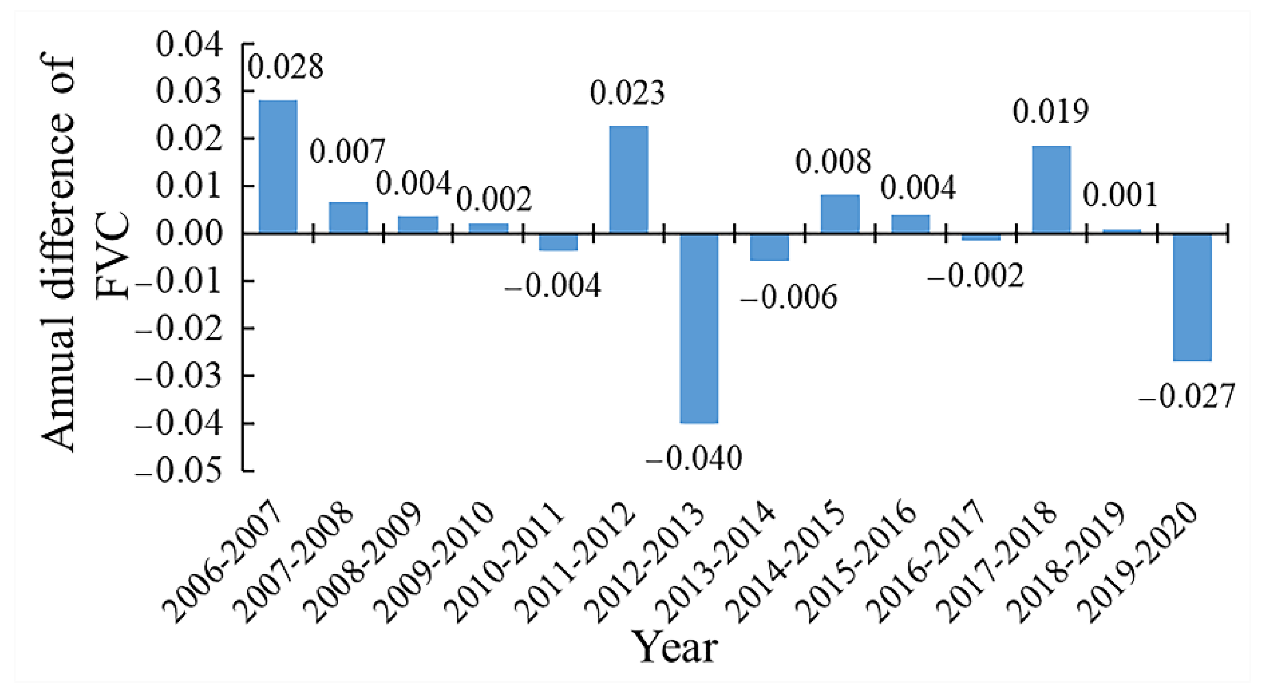
2.3.4. Annual Variation Trend of FVC

The univariate linear regression trend analysis method was used, whilst the least square method was used for fitting the slope of the annual average FVC pixel by pixel, simulating the change trend of each grid [37,38]. The Calculation Formula is as follows:

$${\theta }_{slope}=\frac{n\times {\sum }_{i=1}^n(i\times FV{C}_i)-\left({\sum }_{i=1}^{n}i\right)\left({\sum }_{i=1}^{n}FV{C}_i\right)}{n\times {\sum }_{i=1}^n{i}^2-{({\sum }_{i=1}^{n}i)}^2}$$

(14)

where θ_slope is the slope of the change trend of the FVC in the multi-year time series, i is the serial number of the study year, n is the length of the study time series, and FVC_i is the FVC value in the ith year. If θ_slope > 0 indicates that the change trend of FVC is increasing, θ_slope < 0 indicates that the change trend of FVC is decreasing. The significance test of the trend adopts F test, and the significance indicates the reliability of the change trend. According to the test results, the change trend is divided into five grades: extremely significant decrease (θ_slope < 0, p ≤ 0.01); significantly reduced (θ_slope < 0, 0.01 < p ≤ 0.05); there was no significant change (p > 0.05); significant increase (θ_slope> 0, 0.01 < p ≤ 0.05); and extremely significant increase (θ_slope > 0, p ≤ 0.01).

3. Results

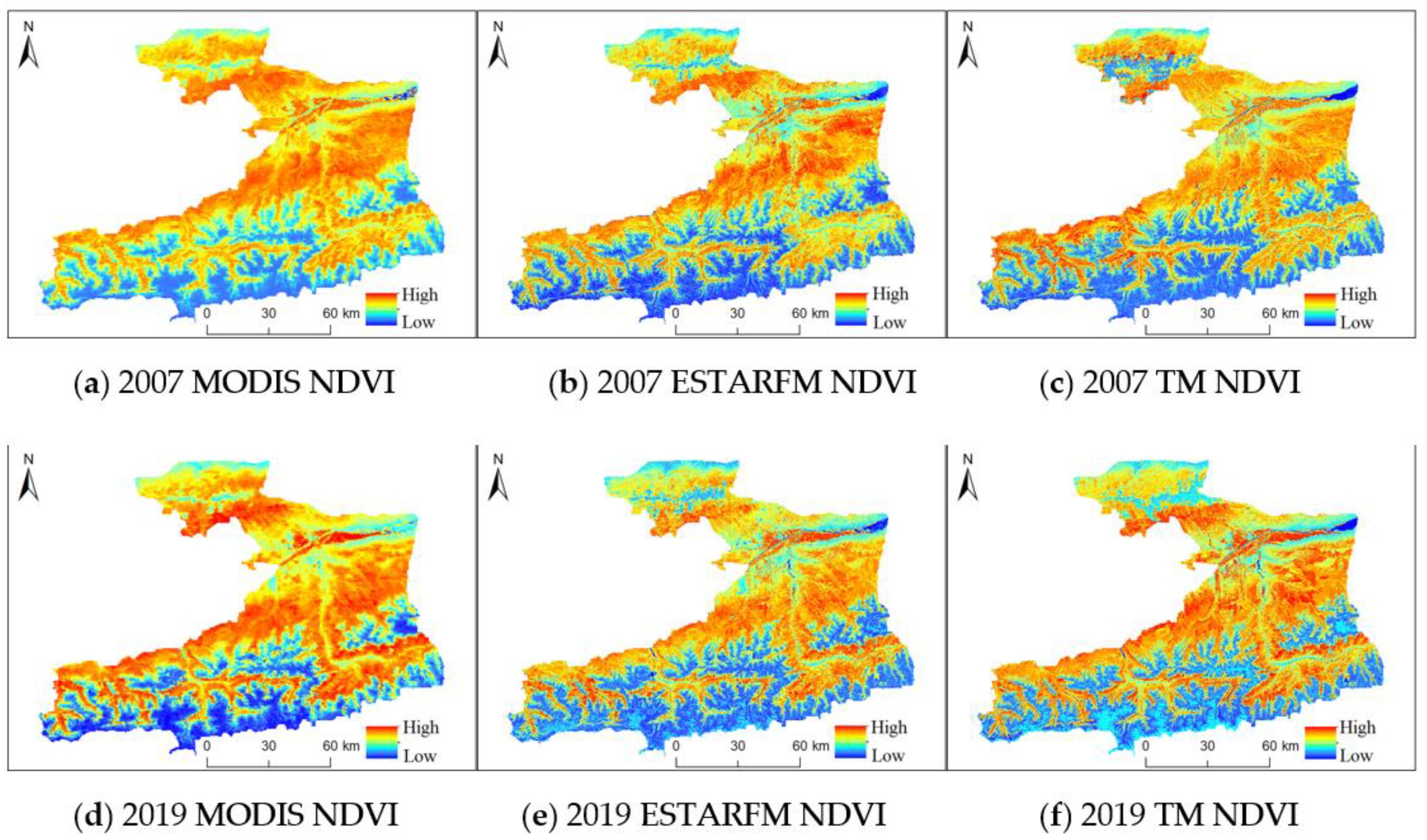
3.1. ESTARFM Model Fusion Results

In order to verify the fusion results of ESTARFM Model, TM NDVI was taken in this paper on 21 June 2007 and 25 September 2007, as well as OLI NDVI on 30 May 2019 and 14 October 2019 and the corresponding MODIS NDVI as an input data. The NDVI data was fused on 13 August 2007 and 13 August 2019, and then compared with the real NDVI data in the corresponding period. Figure 2 is a comparison of the fusion results of the ESTARFM Model. It can be found that compared with MODIS NDVI data through visual interpretation, the spatial resolution of the fused NDVI data is significantly improved; the two data have good consistency compared with TM / OLI NDVI data. Meanwhile, it is found from Figure 2b,c that the NDVI data fused by ESTARFM restores the original spectral information of the cloud cover area.

To further analyze the fusion effect, five typical 100 × 100 image subsets (Figure 3) were selected in this paper, and the fused NDVI data were compared with the real Landsat NDVI data, and a scatter plot was obtained (Figure 4). From Figure 4, it can be seen that the scatter points are basically distributed on both sides of the contour 1:1, indicating that the fused NDVI data are similar to the real NDVI data, and the determination coefficients of the fused NDVI data and the real NDVI data in the two scenes are 0.86 and 0.88, and the root mean square errors are 0.15 and 0.12, respectively, with high correlation. Therefore, the NDVI data obtained by fusion based on the ESTARFM model can be used for the estimation of secondary vegetation.

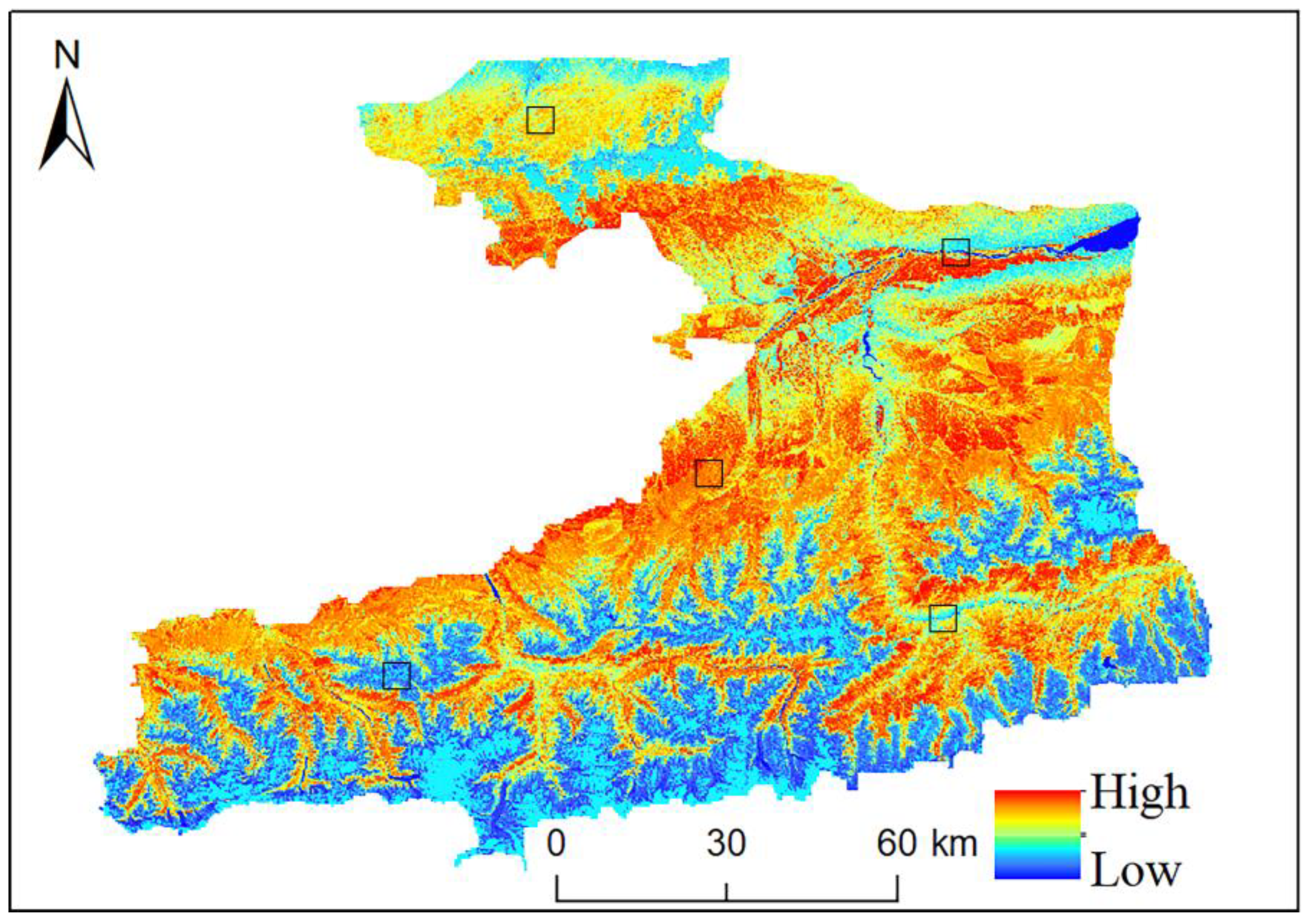
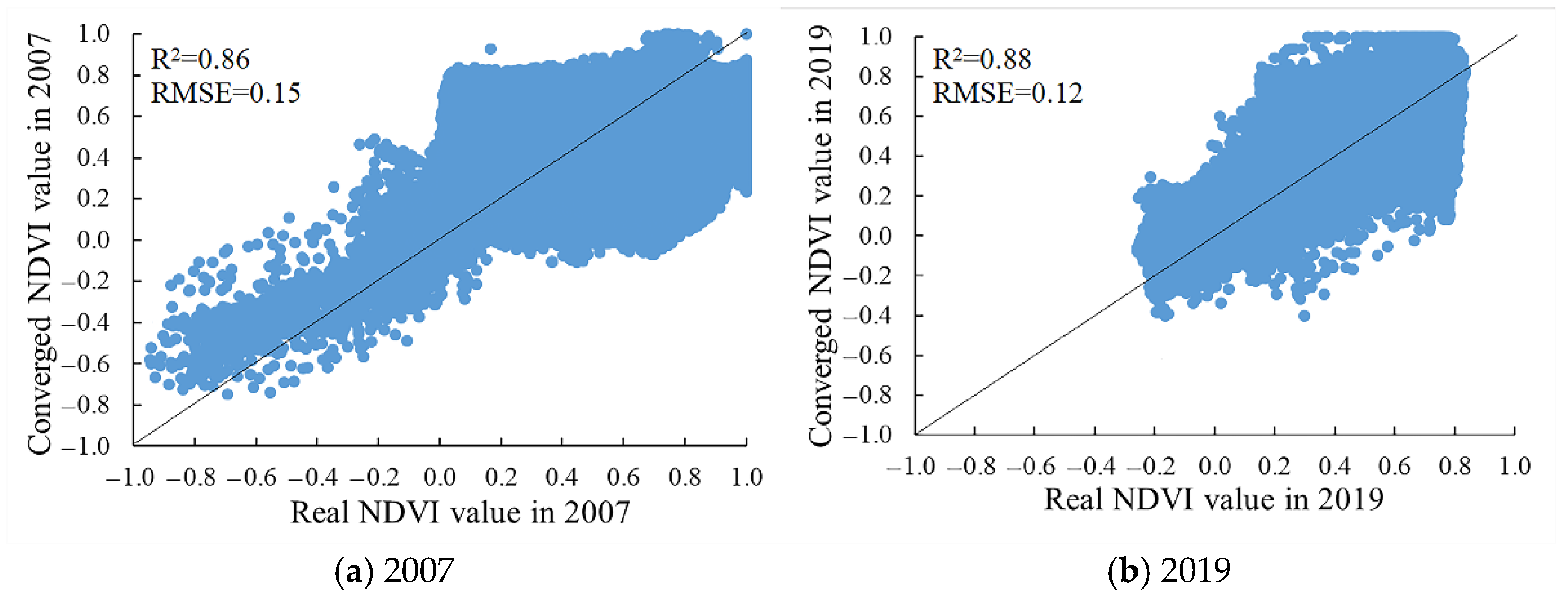
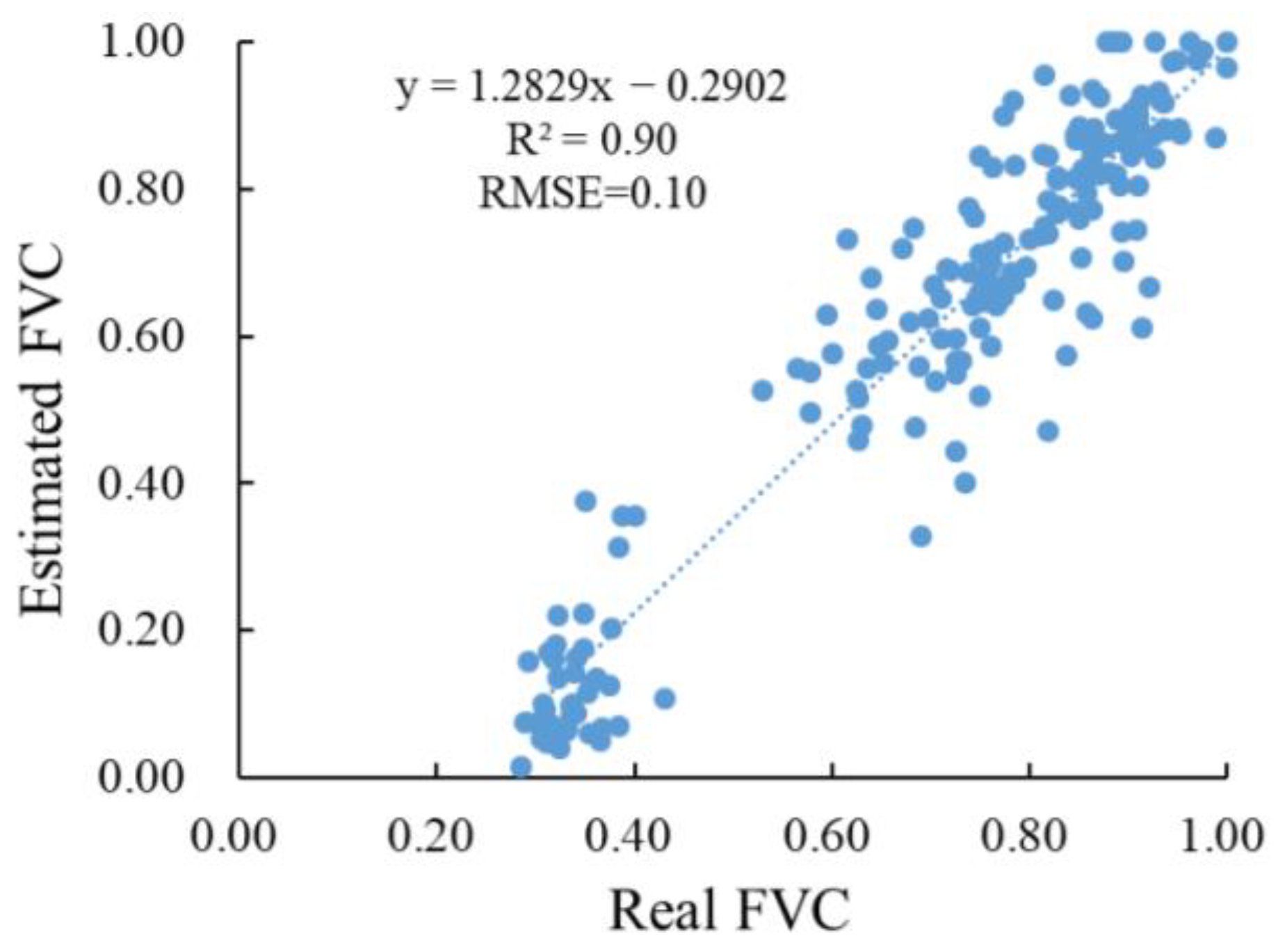
3.2. FVC Accuracy Verification

The accuracy verification results (Figure 5) show that the RMSE between the estimated value of the pixel binary model and the real value is 0.10, whilst the R² is 0.90, indicating that the FVC estimation results of Landsat data using the pixel binary model have a high accuracy and meet the requirements of this study.

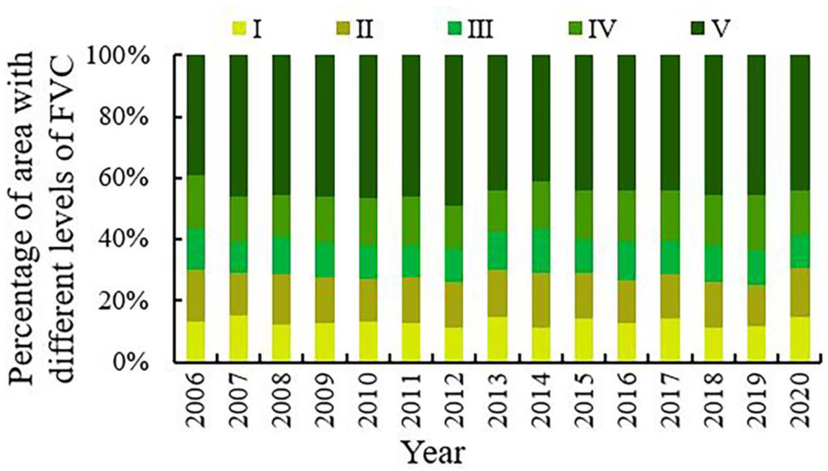
3.3. Temporal and Spatial Variation Characteristics of FVC

Figure 6 shows the inter annual difference of FVC, which is the average of the difference of FVC every two years in the study time series to analyze its inter annual change degree. As can be seen from Figure 6, FVC showed an increasing trend from 2006 to 2010; except for 2012, FVC showed a decreasing trend from 2011 to 2014; except for 2017, FVC showed an increasing trend from 2015 to 2019; and in 2020, it showed a decreasing trend again. Among them, the largest increases and decreases were in 2007 (0.028) and 2013 (−0.040), respectively.

As shown in Figure 7, through statistical analysis of FVC at all levels in the study area, it can be found that from 2006 to 2020, the proportion of high FVC area in the study area showed a law of increase-decrease-increase, reaching a minimum of about 38% in 2006 and a maximum of about 49% in 2012; the proportion of medium high and medium FVC area showed a trend of decrease-increase- decrease, with the minimum proportions of 13% in 2013 and 9% in 2007, and the maximum proportion of 18% in 2019 and 14% in 2014; the area proportion of low and very low FVC changes in a wave pattern, and is stable between 14~16% and 12~14%, respectively. The high, medium high, medium, low and extremely low FVC accounts for 45%, 18%, 11%, 14% and 12% of the total area of the study area respectively according to the 15 years of average FVC. In general, the proportion of high FVC area is the largest and shows an increasing trend, the proportion of medium, high and medium FVC area shows a fluctuating and decreasing trend, and the proportion of low and very low FVC area shows a wavy change.

As shown in Figure 8, it can be found that the regional difference of average FVC in the study area is significant. The overall FVC in the north and central Tex River Valley is high, while the overall FVC in the southern mountainous area is low, and only the river valley has a high FVC. This is because the overall altitude of the southern mountainous area is high, and there are glaciers and snow, which are inhospitable to vegetation growth. The vegetation cover was counted in the forestry administrative district, and the results showed that: the best vegetation cover was in Tex, with an average FVC of 0.62; the second best vegetation cover was in Qapqal, with an average FVC of 0.6; and the vegetation cover in Zhaosu was relatively poor, with an average FVC of 0.47.

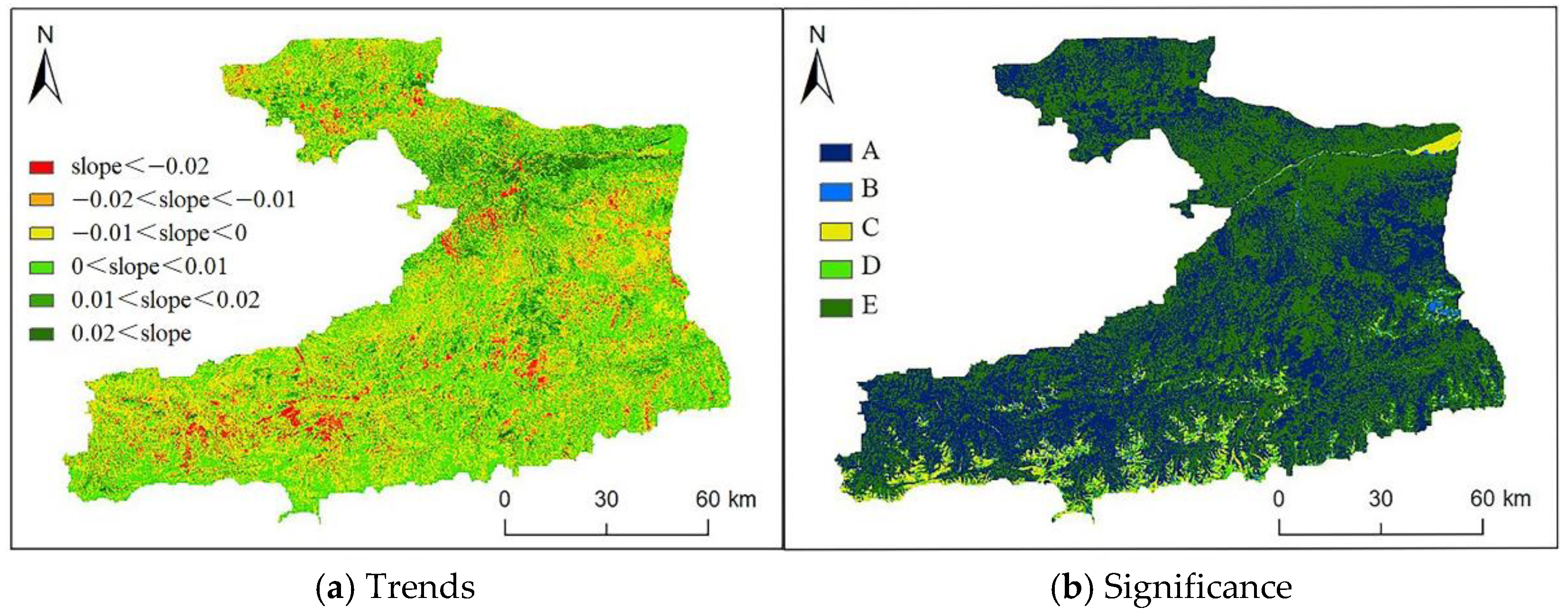
3.4. Slope Change Trend of FVC

The change trend of FVC in the Western Tianshan Mountains from 2006 to 2020 is analyzed at the pixel scale, and the results are tested for significance (Figure 9,

Table 2. Vegetation cover change and significance statistics.

Slope	Percentage/%	Significance	Percentage/%
Slope < −0.02	3.7%	Extremely significant decrease	43%
−0.02 < Slope < −0.01	9.7%	Significant decrease	2.1%
−0.01 < Slope < 0	34.3%	Insignificant change	6%
0 < Slope < 0.01	38%	Significant increase	3.3%
0.01 < Slope < 0.02	10.4%	Extremely significant increase	45.6%
Slope > 0.02	3.9%

) based on the univariate linear regression model. The average change trend of FVC in the Western Tianshan region is 0.3%/10A, indicating that the overall FVC in the Western Tianshan Region is increasing, but the growth rate is relatively slow. The proportion of areas with positive and negative slope is 52.3% and 47.7%, respectively. Among the pixels with decreasing FVC, the proportion of pixels with larger decreasing trend (slope < −0.01) is 28%, and the proportion of pixels with larger increasing trend (slope > 0.01) is 27%. The results of significance test (Figure 9b) show that the FVC in the Western Tianshan Mountains shows extremely significant decrease, significant decrease, no significant change, significant increase and extremely significant increase, accounting for 43%, 2.1%, 6%, 3.3% and 45.6%, respectively. It can be found that there is a large area and a high degree of vegetation improvement and degradation in the Western Tianshan Region, and its area proportion and change degree are basically the same as the degradation phenomenon. This also makes the vegetation change in the Western Tianshan Region show an insignificant trend generally, but its internal changes are quite different.

Compared with Figure 8, it can be found that the insignificant changes are mainly in the extremely low FVC area, which is also the glacier snow coverage area, and the interference of human activities is small; the extremely significant increase mainly occurs in the low and medium FVC areas, and the extremely significant decrease mainly occurs in the medium high and high FVC areas, which changes are mainly affected by global climate change and human disturbance.

3.5. Distribution and Variation Characteristics of FVC with Terrain

The growth and spatial distribution of vegetation are affected by climate, topography, and human activities, among which the topographic factors affect the growth of vegetation by changing the vegetation habitat elements such as water, heat, and soil in local areas. In this study, concerning desertification land and plain forest resources investigation, the altitude, slope and aspect are divided into 7, 6 and 9 grades according to the classification standard of the data dictionary of Xinjiang desertification, and then the distribution and change of FVC in the study area in the past 15 years under different terrain conditions are statistically analyzed. The results are shown in Figure 10, Figure 11 and Figure 12.

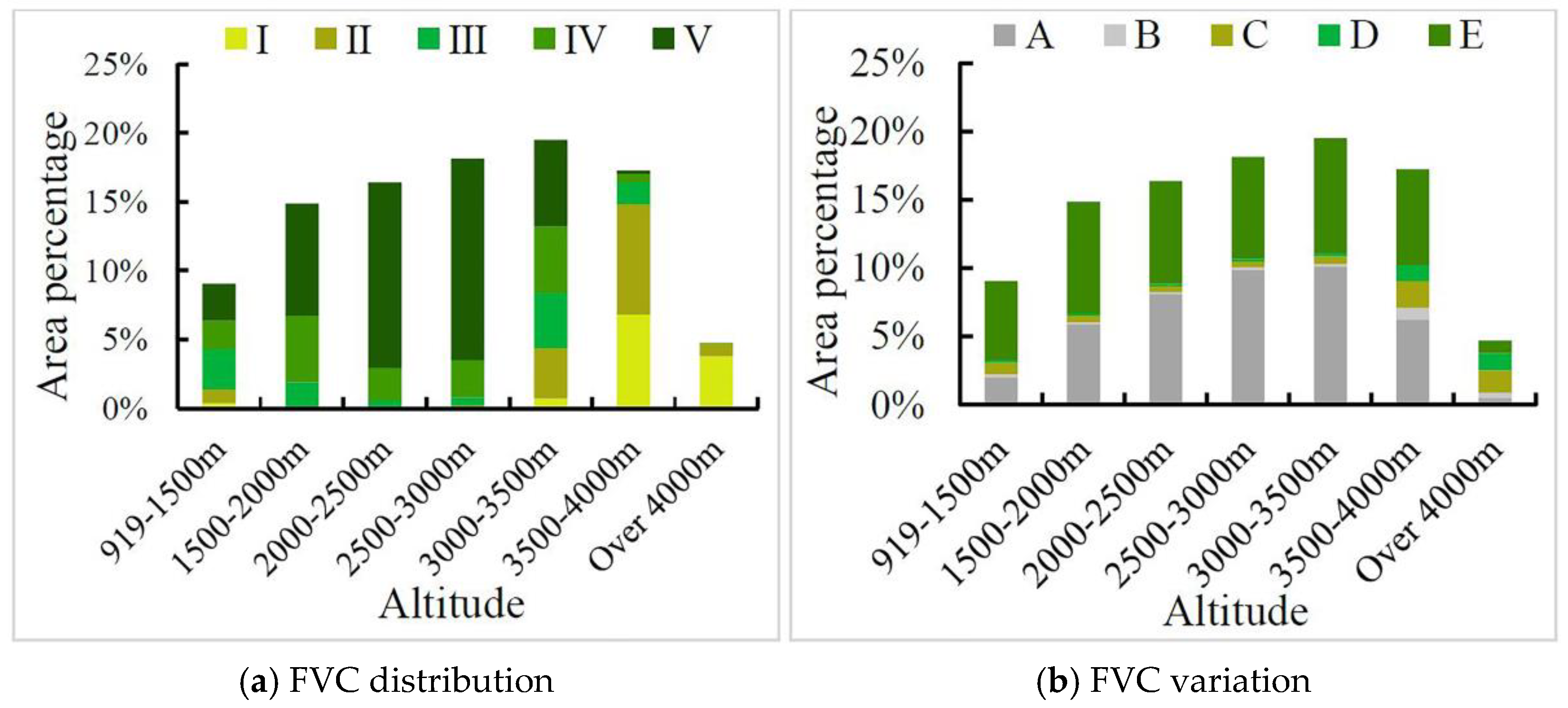
3.5.1. Distribution and Variation Characteristics of FVC with Altitude

As shown in Figure 10a, the vegetation was mainly distributed in the area from 1500 to 4000 m, accounting for 86% of the total vegetation area in the study area. Among them, the area of high FVC increases with altitude below 3000 m and is absolutely dominant; in the area from 3000 to 4000 m, the area of very low and low FVC shows an increasing trend, and in the area above 4000 m, the vegetation decreases rapidly and is dominated by very low FVC, which is mainly influenced by natural conditions. As shown in Figure 10b, the change of vegetation cover is mainly in the area below 4000 m, which is related to the vegetation distribution. In the area from 2000 to 3500 m, the proportion of decrease in vegetation cover is greater than the proportion of increase, indicating a slight degradation trend of vegetation cover in this elevation range; in the remaining elevations, the proportion of increase in vegetation cover is higher than the proportion of decrease, indicating a slight improvement trend of vegetation cover in this elevation range. The area above 4000 m is less affected by human activities, and is mainly an insignificant change.

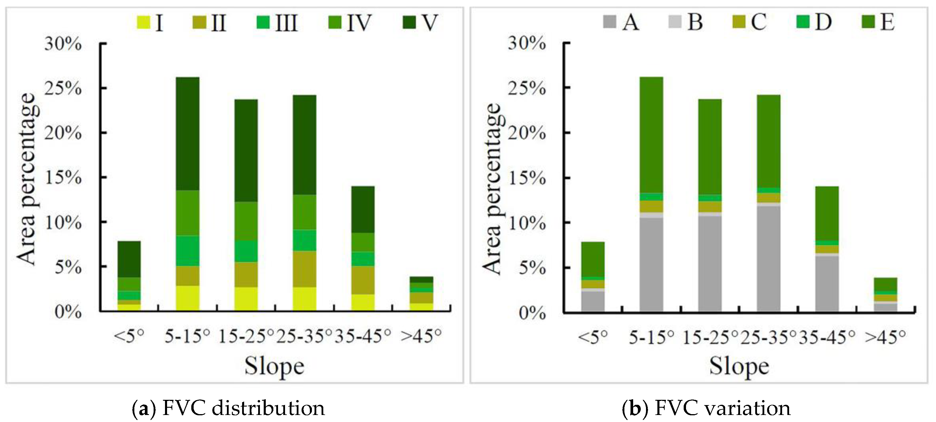
3.5.2. Distribution and Variation Characteristics of FVC with Slope

As shown in Figure 11a, the vegetation was mainly distributed in the area from 5° to 45°, accounting for 88% of the total vegetation coverage in the study area. In each slope class, the proportion of high and medium-high FVC area gradually decreases and the proportion of very low and low FVC area gradually increases as the slope increases; except for >45° slope class, high FVC occupies absolute dominance in all slope classes. As shown in Figure 11b, corresponding to the distribution of vegetation in different slope grades, the changes of FVC are also mainly distributed in the area from 5° to 45°. In each slope class, significant decrease, insignificant change and significant increase were basically maintained in low proportions. In the slope range from 25° to 45°, the proportion of decrease in vegetation cover was greater than the proportion of increase, indicating a slight degradation trend of vegetation cover in this slope range; in the rest of the slope classes, the proportion of increase in vegetation cover was greater than the proportion of decrease, indicating a slight improvement trend of vegetation cover in this slope range.

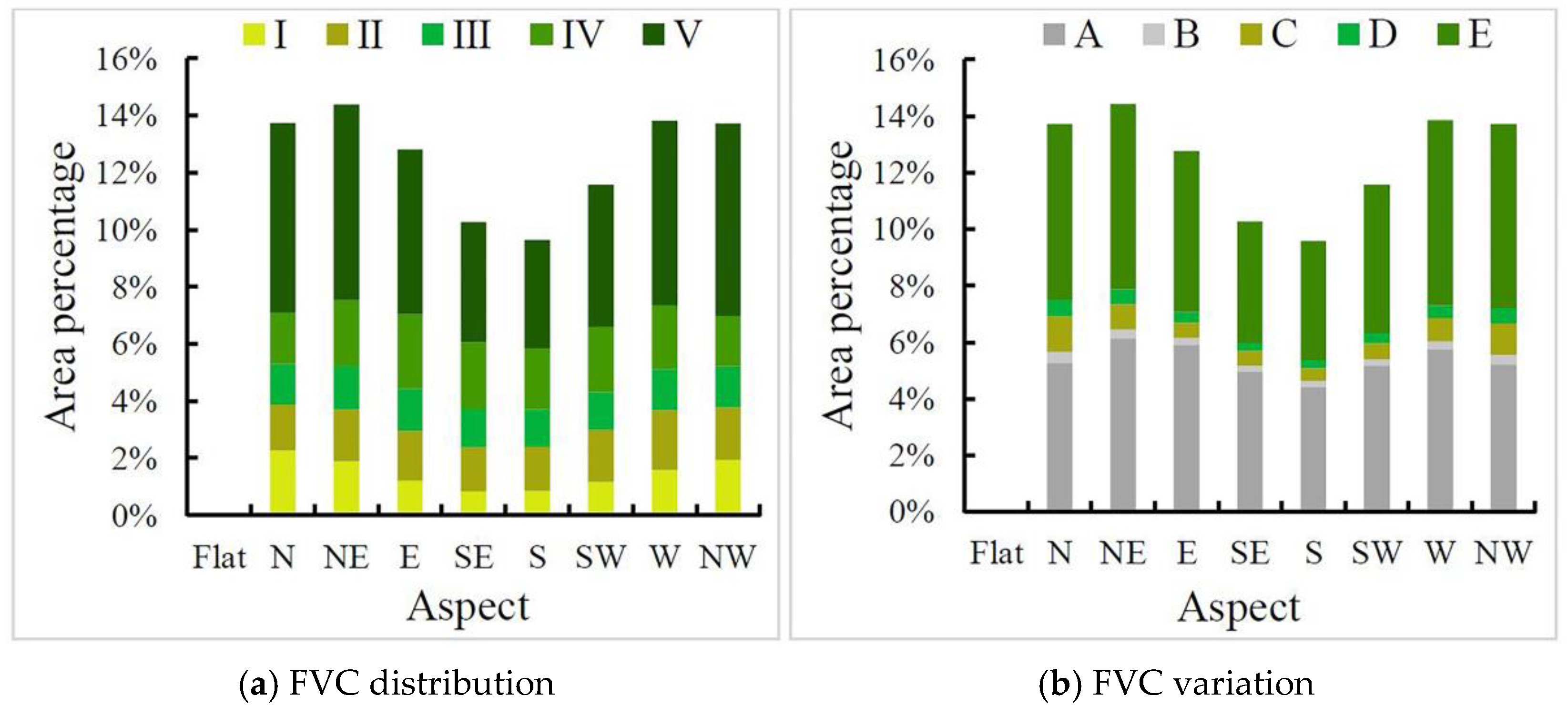
3.5.3. Distribution and Variation Characteristics of FVC with Direction

As shown in Figure 12a, the vegetation cover of flat slopes only accounted for 0.05% of the total vegetation cover in the study area, and the difference in the proportion of vegetation distribution in the remaining slope directions was small. Among the slope directions, the vegetation distribution area is higher on the north slope than on the south slope, and higher on the west slope than the east slope. This is because the north and west slopes are windward slopes in the western Tian Shan region, which have more precipitation and a more humid environment suitable for the growth of vegetation. As shown in Figure 12b, the distribution of vegetation change in the flat slope area is the least, and the difference of the distribution ratio of vegetation change in the remaining slope directions is small, which is closely related to the distribution of vegetation. Among the slopes, the decrease proportion of vegetation in the south and southeast slopes is larger than the increase proportion, which indicates that the vegetation cover in the south and southeast shows a slight trend to degradation; the increase proportion of vegetation in the rest of the slopes is larger than the decrease proportion, which indicates that the vegetation cover in these slopes shows a slight trend to improvement.

4. Discussion

In studies related to vegetation cover change in arid and semi-arid areas of Xinjiang, China, low spatial resolution time series data such as MODIS NDVI (16 d/250 m/500 m) [21,22] and GIMMS NDVI (15 d/8 km) [23,24,25] are mostly used. Among them, MODIS data are used in vegetation cover change studies after 2000, and longer time scale data are dominated by GIMMS data. Other scholars have used Landsat data for vegetation cover change studies with higher spatial resolution in a 5-year span [18,19]. However, studies based on the above data require a trade-off between temporal continuity and spatial resolution, and cannot achieve long time series to monitor vegetation change trends with high accuracy. In a study by Cai et al. [21] based on MODIS data, vegetation degradation occurred in the Tianshan region of Xinjiang in 2013 and 2014, and vegetation grew rapidly again in 2015, while no abrupt change years were found in a study by Wen et al. [18] with a 5-year span of Landsat data. In this paper, the time-series data obtained based on ESTARFM model can also detect the vegetation degradation in 2013 and 2014 years while having high spatial resolution. On the other hand, in the West Tianshan region, where the topography is complex and the terrain is undulating, low-resolution remote sensing data often produces large errors when analyzing the influence of each topographic factor on vegetation cover [39]. In this paper, we effectively obtained the high-spatial resolution time-series NDVI data based on ESTARFM model for the complex terrain area in the western Tianshan Mountains, which provides data support to realize the dynamic monitoring of cover change in the complex terrain area in the western Tianshan Mountains.

In this paper, we conducted a study on vegetation cover change based on ESTARFM NDVI data and found that the overall FVC in the western Tian Shan showed a weak increasing trend, which was strongly associated with ecological restoration projects implemented by the Chinese government in recent years, but a degradation trend was observed in the years 2013, 2014, and 2020, indicating that the ecological environment is vulnerable to disturbance by natural and human activities [18,19,23]. It was also found that while the overall FVC in the study area showed an increase, there was a large variation in the internal changes and a large area of improvement and degradation at the same time, which is basically consistent with previous studies [18,40,41,42]. Compared with the study by Wang et al. [43], the different criteria for classifying the trend level of change and the difference in the resolution of remote sensing data make the results of the study somewhat different. In the river valley and pre-mountain plain zone, it is mainly a medium vegetation cover area, where water and heat conditions and topography are suitable and human activities are concentrated, presenting a medium vegetation cover with a strong vegetation change trend at the same time. With the increase of altitude, the increase of snow and ice melt water, and the decrease of human activities, the vegetation shows high vegetation cover and the vegetation change trend gradually decreases. The southern part of the study area is the summit part of Tianshan Mountain, where the vegetation cover is low because of the high altitude and the snow and glacier cover above the snow line, which is not suitable for vegetation growth. At the same time, the natural and human influences in this area are less variable, which makes the vegetation change in this area extremely insignificant.

Influenced by Atlantic water vapor, the West Tianshan region receives more precipitation and is one of the regions with rich forest resources in Xinjiang. However, due to the temperate continental semi-arid climate, the ecological environment is fragile, and the degradation of vegetation still occurs in some areas under the influence of climate change and human activities. The elevation range of vegetation degradation is from 2000 to 3500 m, the slope is from 25° to 45°, and the slope direction is south and southeast slope. Human activities are one of the reasons for the degradation of vegetation in this area. Early urban expansion and construction of aqueducts destroyed the original landscape ecology, resulting in a fragile ecological environment with poor self-repair ability, which in turn led to a long-term trend of weak degradation. On the other hand, the influence of each topographic factor on the change of vegetation cover is complex and comprehensive, and the growth and spatial location of vegetation are closely related to the geographical environment. Elevation, slope, and slope direction determine the distribution of vegetation in mountainous areas by influencing the distribution of water and heat. In areas with slopes greater than 25°, precipitation and ice melt water are not easily stored, soil erosion is serious, and the soil is infertile, resulting in a more fragile vegetation ecology, and the ecological management effect is often unsatisfactory, which is the focus of environmental and ecological management projects [44].

5. Conclusions

Based on the ESTARFM model, this paper fused Landsat and MODIS data to obtain the time-series NDVI data of the study area for the past 15 years and estimated the FVC. Through trend analysis and combining with DEM data, the characteristics of FVC changes in the study area and its response to topographic factors were studied, and the main conclusions are as follows:

(1) The time-series NDVI data of the study area obtained by using ESTARFM Model can not only greatly improve the spatial resolution, but also better maintain the original spectral information. It has high consistency compared with the real NDVI data, indicating that the ESTARFM Model can better simulate the high spatial resolution NDVI data in the missing phase, which can monitor and study the dynamic change of vegetation cover in the complex terrain area of Xinjiang in a long time series.

(2) The overall vegetation cover of the study area was at a high level from 2006 to 2020, and the average annual vegetation cover showed a weak increasing trend in fluctuation. Among all FVC levels, the area with high FVC accounts for the largest, with an average of 45% for many years, and it is generally increasing; the proportion of medium high and medium FVC area showed a fluctuating and decreasing trend; the area proportion of low and very low FVC changes in waves. In terms of spatial distribution, there are obvious regional differences, showing the distribution characteristics of high in the north and low in the south.

(3) From the change trend of FVC, the area with improved FVC in the study area in the past 15 years is larger than the area with degraded FVC, accounting for 52.3% and 47.7%, respectively. The results of significance test show that the areas with no significant changes are mainly concentrated in the extremely low FVC area, i.e., the southern part of the study area is also the glacier snow coverage area with less interference from human activities; the extremely significant increase mainly occurred in the low and medium FVC areas, and the extremely significant decrease mainly occurred in the medium high and high FVC areas.

(4) According to different terrain conditions, the main distribution areas of vegetation cover are 1500–4000 m above sea level, 5°–45° slope and all slope directions except flat slope; the areas with a slight degradation trend of FVC are mainly 2000–3500 m above sea level, 25°–45° slope and south and southeast slope, while the FVC in other areas showed a slight improvement trend.

References

1. Dixon, R.K.; Brown, S.; Houghton, R.A.; Solomon, A.M.; Trexler, M.C.; Wisniewski, J. Carbon pools and flux of global forest ecosystems. Science 1994, 263, 185–190. [Google Scholar] [CrossRef] [PubMed]
2. Sitch, S.; Smith, B.; Prentice, I.C.; Arneth, A.; Bondeau, A.; Cramer, W.; Kaplans, J.O.; Levis, S.; Lucht, W.; Sykes, M.T.; et al. Evaluation of ecosystem dynamics, plant geography and terrestrial Carbon cycling in the LPJ dynamic global vegetation mode. Glob. Change Biol. 2003, 9, 161–185. [Google Scholar] [CrossRef]
3. Wu, X.R.; Guo, P.; Sun, Y.Q.; Liang, H.; Zhang, X.G.; Bai, W.H. Recent Progress on Vegetation Remote Sensing Using Spaceborne GNSS-Reflectometry. Remote Sens. 2021, 13, 4244. [Google Scholar] [CrossRef]
4. Hao, J.W.; Chu, L.M. Vegetation Types Attributed to Deforestation and Secondary Succession Drive the Elevational Changes in Diversity and Distribution of Terrestrial Mosses in a Tropical Mountain Forest in Southern China. Forests 2021, 12, 961. [Google Scholar] [CrossRef]
5. Parmesan, C.; Yohe, G. A globally coherent fingerprint of climate change impacts across natural systems. Nature 2003, 421, 37–42. [Google Scholar] [CrossRef]
6. Yu, L.X.; Yan, Z.R.; Zhang, S.W. Forest Phenology Shifts in Response to Climate Change over China–Mongolia–Russia International Economic Corridor. Forests 2020, 11, 757. [Google Scholar] [CrossRef]
7. Notaro, M.; Mauss, A.; Williams, J.W. Projected vegetation changes for the American Southwest: Combined dynamic modeling and bioclimatic-envelope approach. Ecol. Appl. 2012, 22, 1365–1388. [Google Scholar] [CrossRef]
8. Yang, X.C.; Xu, B.; Jin, Y.X.; Qin, Z.H.; Ma, H.L.; Li, J.Y.; Zhao, F.; Chen, S.; Zhu, X.H. Remote sensing monitoring of grassland vegetation growth in the Beijing–Tianjin sandstorm source project area from 2000 to 2010. Ecol. Indic. 2015, 51, 244–251. [Google Scholar] [CrossRef]
9. Wang, J.; Xie, Y.W.; Wang, X.Y.; Guo, K.M. Driving factors of recent vegetation changes in Hexi Region, Northwest China based on a new classification framework. Remote Sens. 2020, 12, 1758. [Google Scholar] [CrossRef]
10. Hill, M.J.; Guerschman, J.P. Global trends in vegetation fractional cover: Hotspots for change in bare soil and non-photosynthetic vegetation. Agric. Ecosyst. Environ. 2022, 324, 107719. [Google Scholar] [CrossRef]
11. Gitelson, A.A.; Kaufman, Y.J.; Stark, R.; Rundquist, D. Novel algorithms for remote estimation of vegetation fraction. Remote Sens. Environ. 2002, 80, 76–87. [Google Scholar] [CrossRef] [Green Version]
12. Zhang, J.; Walsh, J.E. Relative impacts of vegetation coverage and leaf area index on climate change in a greener north. Geophys. Res. Lett. 2007, 34, L15703. [Google Scholar] [CrossRef]
13. Song, Y.F.; Guo, Z.X.; Lu, Y.J.; Yan, D.H.; Liao, Z.L.; Liu, H.W.; Cui, Y.J. Pixel-Level Spatiotemporal Analyses of Vegetation Fractional Coverage Variation and Its Influential Factors in a Desert Steppe: A Case Study in Inner Mongolia, China. Water 2017, 9, 478. [Google Scholar] [CrossRef]
14. Smith, A.M.S.; Kolden, C.A.; Tinkham, W.T.; Talhelm, A.F.; Marshall, J.D.; Hudak, A.T.; Boschetti, L.; Falkowski, M.J.; Greenberg, J.A.; Anderson, J.W.; et al. Remote sensing the vulnerability of vegetation in natural terrestrial ecosystems. Remote Sens. Environ. 2014, 154, 322–337. [Google Scholar] [CrossRef]
15. Liu, D.Y.; Jia, K.; Jiang, H.Y.; Xia, M.; Tao, G.F.; Wang, B.; Chen, Z.L.; Yuan, B.; Li, J. Fractional Vegetation Cover Estimation Algorithm for FY-3B Reflectance Data Based on Random Forest Regression Method. Remote Sens. 2021, 13, 2165. [Google Scholar] [CrossRef]
16. Phiri, D.; Morgenroth, J. Developments in Landsat Land Cover Classification Methods: A Review. Remote Sens. 2017, 9, 967. [Google Scholar] [CrossRef] [Green Version]
17. Wang, Y.L.; Li, M.S. Annually Urban Fractional Vegetation Cover Dynamic Mapping in Hefei, China (1999–2018). Remote Sens. 2021, 13, 2126. [Google Scholar] [CrossRef]
18. Wen, G.C.; Zhao, M.J.; Xie, H.B.; Zhang, Y.; Zhang, j. Analysis of land vegetation cover evolution and driving forces in the western part of the Ili River Valley. Arid Zone Res. 2021, 38, 843–854. [Google Scholar]
19. Li, H.M.; Bahejiayinaer, T.; Chang, S.L.; Zhang, Y.T. Spatial-temporal change and prediction analysis of vegetation coverage in the northern slope of Tianshan Mountains in 30 years. Chin. J. Ecol. 2022, 1–15. Available online: http://kns.cnki.net/kcms/detail/21.1148.q.20220526.1759.025.html (accessed on 16 November 2022).
20. Chang, M.D.; Wang, X.J.; Yan, L.N.; Ma, K.; Li, Y.K.; Li, J.Y.; Jia, H.T. Temporal and spatial pattern dynamic variations of vegetation cover and management factors in the middle of the northern slope of Tianshan Mountains. J. Agric. Res. Environ. 2022, 39, 836–846. [Google Scholar]
21. Cai, C.C.; Huai, Y.J.; Bai, T.; Dong, L. Recent Changes of Grassland Cover in Xinjiang Based on NDVI Analysis. J. Basic Eng. 2020, 28, 1369–1381. [Google Scholar]
22. Yin, Z.L.; Feng, Q.; Wang, L.G.; Chen, Z.X.; Chang, Y.B.; Zhu, R. Vegetation coverage change and its influencing factors across the northwest region of China during 2000–2019. J. Desert Res. 2022, 42, 11–21. [Google Scholar]
23. Wang, H.J.; Li, Z.; Niu, Y.; Li, X.C.; Cao, L.; Feng, R.; He, Q.N.; Pan, Y.P. Evolution and Climate Drivers of NDVI of Natural Vegetation during the Growing Season in the Arid Region of Northwest China. Forests 2022, 13, 1082. [Google Scholar] [CrossRef]
24. Li, X.W.; Zulkar, H.; Wang, D.Y.; Zhao, T.N.; Xu, W.T. Changes in Vegetation Coverage and Migration Characteristics of Center of Gravity in the Arid Desert Region of Northwest China in 30 Recent Years. Land 2022, 11, 1688. [Google Scholar] [CrossRef]
25. Mu, B.; Zhao, X.; Wu, D.H.; Wang, X.Y.; Zhao, J.C.; Wang, H.Y.; Zhou, Q.; Du, X.Z.; Liu, N.J. Vegetation Cover Change and Its Attribution in China from 2001 to 2018. Remote Sens. 2021, 13, 496. [Google Scholar] [CrossRef]
26. Gao, F.; Masek, J.; Schwaller, M.; Hall, F. On the blending of the Landsat and MODIS surfaces reflectance: Predicting daily Landsat surface reflectance. IEEE Tran. Geosci. Remote Sens. 2006, 44, 2207–2218. [Google Scholar]
27. Zhu, X.L.; Chen, J.; Gao, F.; Chen, X.H.; Masek, J.G. An enhanced spatial and temporal adaptive reflectance fusion model for complex heterogeneous region. Remote Sens. Environ. 2010, 114, 2610–2623. [Google Scholar] [CrossRef]
28. Wu, G.J.; Liu, X.H.; Kang, S.C.; Chen, T.; Xu, G.B.; Zeng, X.M.; Kang, H.H. Age-dependent impacts of climate change and intrinsic water-use efficiency on the growth of Schrenk spruce (Picea schrenkiana) in the western Tianshan Mountains, China. For. Ecol. Manag. 2018, 414, 1–14. [Google Scholar] [CrossRef]
29. Jarihani, A.A.; Mcvicar, T.R.; Vanniel, T.G.; Emelyanova, I.V.; Callow, J.N.; Johansen, K. Blending Landsat and MODIS data to generate multispectral indices: A Comparison of “Index-then-Blend” and “Blend-then-Index” approaches. Remote Sens. 2014, 6, 9213–9238. [Google Scholar] [CrossRef] [Green Version]
30. Xiao, J.F.; Moody, A. A comparison of method for estimating fractional green vegetation cover within a desert-to-upland transition zone in central New Mexico, USA. Remote Sens. Environ. 2005, 98, 237–250. [Google Scholar] [CrossRef]
31. Qi, J.; Marsett, R.C.; Moran, M.S.; Goodrich, D.C.; Heilman, P.; Kerr, Y.H.; Dedieu, G.; Chehbouni, A.; Zhang, X.X. Spatial and temporal dynamics of vegetation in the San Pedro River basin area. Agric. For. Meteorol. 2000, 105, 55–68. [Google Scholar] [CrossRef] [Green Version]
32. Rundquist, B.C. The influence of canopy green vegetation fraction on spectral measurements over native tallgrass prairie. Remote Sens. Environ. 2002, 81, 129–135. [Google Scholar] [CrossRef]
33. Li, M.M. The Method of Vegetation Fraction Estimation by Remote Sensing. Master’s Thesis, University of Chinese Academy of Sciences (Institute of Remote Sensing Applications), Beijing, China, 2003. [Google Scholar]
34. Wei, X.D.; Wang, S.N.; Wang, Y.K. Spatial and temporal change of fractional vegetation cover in North-western China from 2000 to 2010. Geol. J. 2017, 53, 427–434. [Google Scholar] [CrossRef] [Green Version]
35. Wu, C.S.; Murray, A.T. Estimating impervious surface distribution by spectral mixture analysis. Remote Sens. Environ. 2003, 84, 493–505. [Google Scholar] [CrossRef]
36. Suvachananonda, T.; Maruyama, Y. Urban Growth Prediction of Special Economic Development Zone in Mae Sot District, Thailand. Eng. J. 2018, 22, 269–277. [Google Scholar]
37. Zhang, H.; Xue, L.Q.; Wei, G.H.; Dong, Z.C.; Meng, X.Y. Assessing Vegetation Dynamics and Landscape Ecological Risk on the Mainstream of Tarim River, China. Water 2020, 12, 2156. [Google Scholar] [CrossRef]
38. Sun, X.F.; Yuan, L.G.; Zhou, Y.Z.; Shao, H.Y.; Li, X.F.; Zhong, P. Spatiotemporal change of vegetation coverage recovery and its driving factors in the Wenchuan earthquake-hit areas. J. Mt. Sci. 2021, 18, 2854–2869. [Google Scholar] [CrossRef]
39. Qin, J.L.; Xue, L.Q. Spatial and temporal variation characteristics of vegetation in the Manas River Basin in northwest arid region and its spatial relationship with topographical factors. Ecol. Environ. Sci. 2020, 29, 2179–2188. [Google Scholar]
40. Shao, S.S.; Shi, Q.D. Spatial and temporal change of vegetation cover in Xinjiang based on FVC. Sci. Silvae Sin. 2015, 51, 35–42. [Google Scholar]
41. He, B.Z.; Ding, J.L.; Zhang, Z.; Ghulam, A. Experimental analysis of spatial and temporal dynamics of fractional vegetation cover in Xinjiang. Acta Geogr. Sin. 2016, 71, 1948–1966. [Google Scholar]
42. Mo, K.L.; Chen, Q.W.; Chen, C.; Zhang, J.Y.; Wang, L.; Bao, Z.X. Spatiotemporal variation of correlation between vegetation cover and precipitation in an arid mountain-oasis river basin in northwest China. J. Hydrol. 2019, 574, 138–147. [Google Scholar] [CrossRef]
43. Wang, H.L.; Feng, A.P.; Gao, Y.H.; Wang, X.L. Temporal-spatial dynamic change on maximum vegetation coverage degree of Ili River basin. Environ. Sci. Technol. 2018, 41, 161–167. [Google Scholar]
44. He, Z.H.; Zhang, Y.H.; He, Y.; Zhang, X.W.; Cai, J.Z.; Lei, L.P. Trends of Vegetation Change and Driving Factor Analysis in Recent 20 Years over Zhejiang Province. Ecol. Environ. Sci. 2020, 29, 1530–1539. [Google Scholar]
Figure 1. The location and topographic features of the study area, (a) in China, (b) in Xinjiang Uygur Autonomous Region and (c) are topographic features of the study area, and elevation data were obtained from ASTER Global Digital Model.
Forests 13 02066 g001
Figure 2. Comparison of ESTARFM model fusion results.
Forests 13 02066 g002
Figure 3. Distribution of 5 typical image subsets.
Forests 13 02066 g003
Figure 4. Scatter plot of fused NDVI and real NDVI and correlation coefficient.
Forests 13 02066 g004
Figure 5. Comparison of estimated FVC and real FVC.
Forests 13 02066 g005
Figure 6. Annual FVC variance chart.
Forests 13 02066 g006
Figure 7. Interannual variation of different classes of vegetation, where I is Very Low FVC; II is Low FVC; III is Medium FVC; IV is Medium High FVC; V is High FVC. This is the same in Figure 8.
Forests 13 02066 g007
Figure 8. Spatial Distribution of Annual Average FVC in West Tianshan Mountains in the Past 15 Years.
Forests 13 02066 g008
Figure 9. Trends (a) and significance (b) of vegetation cover changes in the western Tian Shan region in the last 15 years, where A is a extremely significant decrease; B is a significant decrease; C is no significant change; D is a significant increase; and E is a significant increase. This is the same in Table 2.
Forests 13 02066 g009
Figure 10. Distribution (a) and variation (b) of FVC at different altitudes.
Forests 13 02066 g010
Figure 11. Distribution (a) and variation (b) of FVC for different slopes.
Forests 13 02066 g011
Figure 12. Distribution (a) and variation (b) of FVC for different slope directions.
Forests 13 02066 g012