Recreational Services from Green Space in Beijing: Where Supply and Demand Meet?

Abstract

Green space, mainly forests, shrubs, and grasslands, provides essential ecosystem services for human well-being. Based on multi-source data and using the Maximum Entropy model and Geographical Information System (GIS) tools, this research comprehensively assesses the supply and demand of recreational services from green space in Beijing. The supply of recreational services in Beijing is influenced by natural and human factors, showing large spatial variability. The supply level of mountainous areas with good natural geographical conditions and intact ecological landscape is significantly higher than that of plain areas with reduced vegetation and overexploitation. Residents have a high demand for recreational services in green space landscape and low demand in non-green space landscape. The quantitative balance pattern of supply and demand varies greatly, and most areas show the state of undersupply. The spatial matching pattern of supply and demand varies significantly too, and the mismatch is apparent. Spatial allocation should be more carefully considered than the aggregated supply and demand. Differentiated development strategies such as ecological reshaping, ecological development, restoration, and protection should be implemented for different areas in the future of planning and management in urban green areas. This will optimize and balance the supply-demand matching pattern for recreational services and promote the effective improvement of ecosystem service functions and residents’ ecological welfare.

1. Introduction

Green space plays an important role in improving the living environment for residents and maintaining the balance of the urban ecosystem [1,2]. The rapid development of modern cities has led to increasing demand for leisure and recreational resources and deterioration of the living environment. People have an increasing desire to access and be close to nature.

The recreational services provided by green space are of great significance to improve the welfare of the residents [3]. Cultural services represented by recreational services are mainly non-material benefits arising from human-ecosystem relationships. They cannot be considered as priori products of nature but rather as relational processes that people actively create, express, and transform through interactions with ecosystems [4]. Therefore, it is hard to quantitatively evaluate recreational services [5]. Existing studies have mostly used monetization methods such as the willingness-to-pay method [6], conditional valuation method [7], and travel cost method [8] to quantitatively evaluate the supply and demand of recreational services. Unfortunately, these methods might not pay adequate attention to geographic conditions and could not reveal information on the spatial distribution of the supply and demand, or the interaction between socioeconomic context and physical geographic features.

Ecosystem services are usually public goods and common resources which make the supply and demand difficult to meet by market mechanisms. Recreational services from green space are usually provided by public financial sources, and how the costs and benefits are shared is essential in city planning and political dialogue. For example, we cannot simply ask suburban and rural areas to bear the costs to provide the services mostly demanded by the urban residents. The livability of modern cities depends to a large extent upon urban and peri-urban ecosystems and their services and emphasizes that these services are not only a gift of nature but also provided with costs [9]. Urban political ecology refutes the traditional dichotomy of city and nature. It argues that urban ecosystem services do not only exist outside, but they are also entwined with urban social and political processes [10,11,12]. Therefore, political ecology researchers focus on using historical and geographic approaches to research natural-social phenomena. They pay particular attention to studying who benefits, who pays, and equity among stakeholders [13].

Recreational services from green space are usually location specific and cannot be moved spatially. Analysis of aggregated supply and demand is less meaningful. Interaction between supply and demand for ecosystem services should pay attention the spatial distribution of environmental resources [14]. As a typical ecosystem cultural service, spatial matching of supply and demand is very important for improving residents’ welfare. Many scholars have conducted research in the related area; Burkhard et al. constructed the first supply-demand balance and relationship matrix for ecosystem services [15]; Baró et al. used spatial mapping to analyze the spatial and temporal characteristics of supply and demand for two types of ecosystem services (air purification, outdoor recreation) [16].

This study intended to use geographic information data, POI (Point of Interest) data and visual survey data and construct the Maximum Entropy model to assess and simulate the supply and demand of recreational services from green space in Beijing. The spatial pattern analysis was conducted using GIS tools to identify the supply-demand matching condition. The analysis was combined with the socioeconomic and physical geographic characteristics of different regions to reveal the interrelationship and conflict between nature and society.

2. Materials and Methods

2.1. Study Area

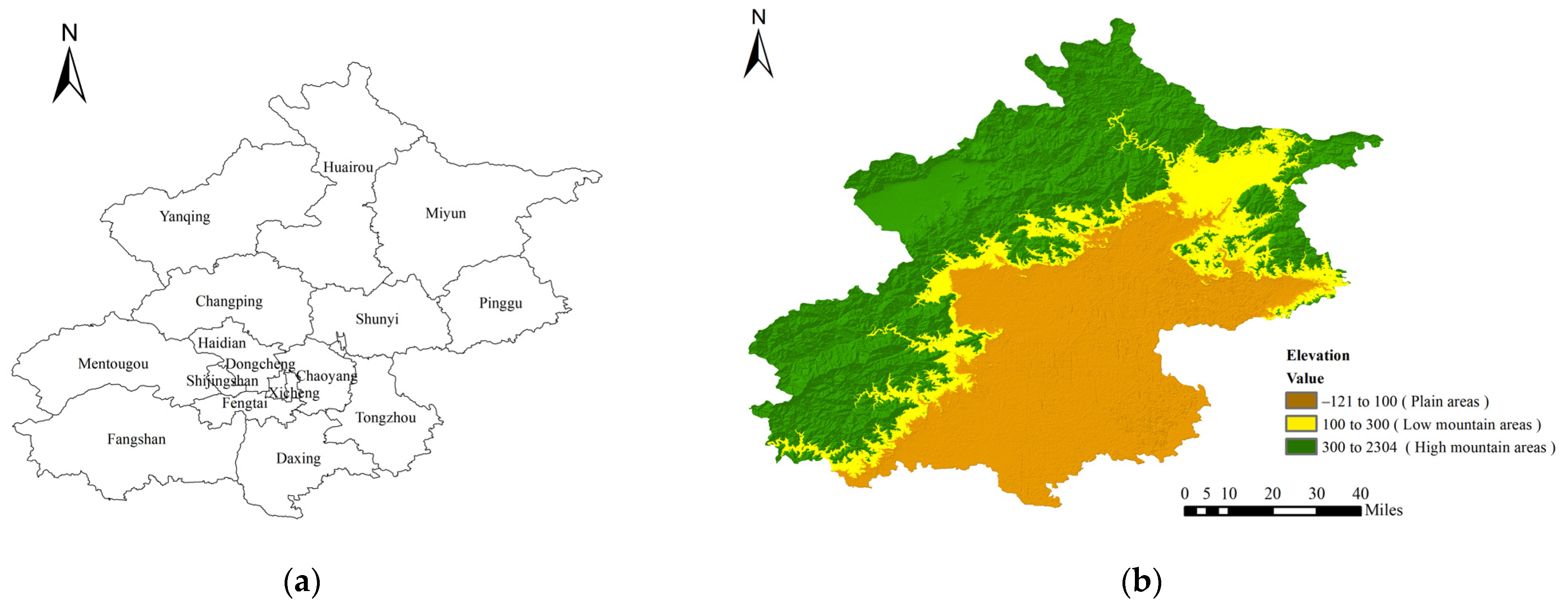
Beijing located in the northern area of China and is the political and cultural center of the country. Beijing has 16 administrative districts (Figure 1a) with a total area of about 16,410 km². In 2019, Beijing had a resident population of about 22 million with an urbanization rate about 87%. The GDP per capita is about USD 25,719.7.

There is a strong demand for recreational services from green space, but the services are mainly allocated to suburban and mountain areas where it is less populated. How to match the supply and demand is very important. To explore this issue in depth, based on Digital Elevation Model (DEM) data (Figure 1b), the study area was divided into mountainous and plain areas according to the urban development plan of Beijing, using 100 m above sea level as the dividing line. The mountainous areas were further subdivided into low mountain areas (elevation from 100 to 300 m) and high mountain areas (elevation >300 m).

2.2. Data Collection

2.2.1. Image Acquisition

Land use data and Digital Elevation Model (DEM) data for Beijing were downloaded from the Resource and Environmental Science and Data Center of the Chinese Academy of Sciences (http://www.resdc.cn, accessed on 10 September 2020). The Land use data was generated based on the Landsat 8 remote sensing images by visual interpretation with a spatial resolution of 30 m; the DEM data were generated based on the SRTM (Shuttle Radar Topography Mission) V4.1 data by resampling with a spatial resolution of 30 m. Vector data of roads, rivers, and lakes in Beijing were downloaded from the National Geographic Information Public Service Platform (http://www.webmap.cn, accessed on 10 September 2020).

Using ArcGIS 10.2 (ESRI, Redlands, CA, USA) as the operating platform, all layers were extracted to the same extent according to the Beijing city boundary and projected to the GCS_WGS_1984 coordinate system. The raster size was set to “30 m × 30 m” and converted to ASCII data format.

2.2.2. POI Data Extraction

Point of Interest (POI) is a geospatial data that represents a real geographic entity and contains information such as name, location, and category. POI data have been attempted to assess and map cultural ecosystem services supply of farmlands [17]. The POI data used in this research were extracted from Baidu Maps (https://lbsyun.baidu.com, accessed on 5 August 2020). Baidu Maps divided the POI data into two levels; the first level industry classification corresponds to industry categories, and the second level industry classification corresponds to geographical entities. According to the original classification of POI, the tags “park”, “scenic area”, “attraction”, “wetland”, “mountain”, “Lake” etc., which are related to recreational services, were selected.

Based on these tags, OSpider_v3.0.0 (https://github.com/skytruine/OSpider, accessed on 5 August 2020) was used to extract POI data from Baidu map. The accuracy of data extraction was limited by the size of the area. The larger the area, the more POI data was missing. Therefore, this study improved the quality of data extraction by setting the initial grid and quadrant threshold. After data cleaning and coordinate conversion and other preprocessing work, we extracted 2477 valid POI data of recreational services.

2.3. Assessment and Mapping the Supply Based on the MaxEnt Model

The Maximum Entropy (MaxEnt) model was used to derive the species’ niche requirements and potential geographic distribution through inductive or simulation analysis of mathematical models. The MaxEnt model can output the probability distribution of an object by exploring the relationship between a set of environmental grids and the location of a given observation point [18]. The greatest advantage of the MaxEnt model is the ability to model presence-only data and to establish complex non-linear relationships between the independent and dependent variables [19]. It is also believed to be robust with small sample sizes [20]. Currently, the MaxEnt model is beginning to be tried by researchers to assess the social value of natural landscape [21].

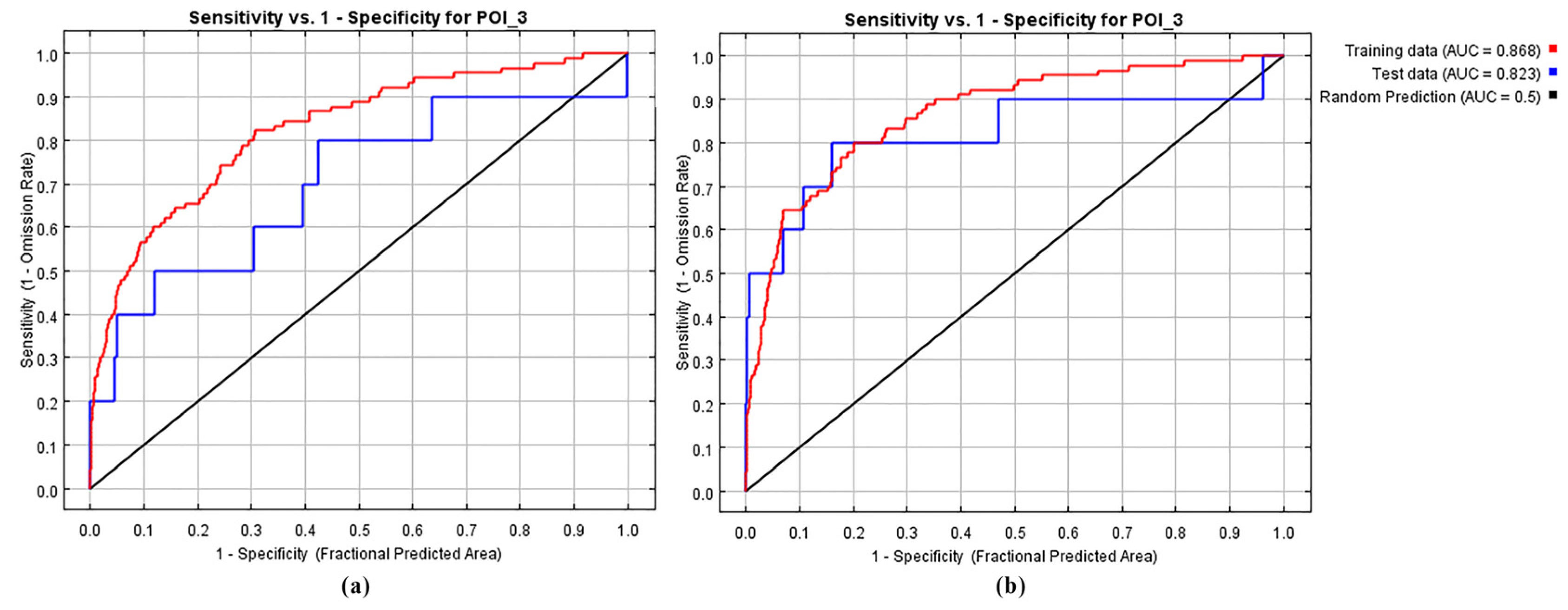
The area under the curve (AUC) of the receiver operating characteristic is widely used to estimate the predictive accuracy of the MaxEnt model. The following criteria are used to judge the accuracy of forecasts: the value of AUC ranges from 0 to 1; 0.9 < AUC ≤ 1 means good effect; 0.7 < AUC ≤ 0.9 means moderate effect; 0.5 < AUC ≤ 0.7 means poor effect [22,23].

To avoid the influence of human or non-green spatial landscape elements on the supply in the urban green space, the scope of this study is based on the composition of land cover types, including woodlands, grasslands, croplands, wetlands, and other green spatial landscape types. The built-up areas such as urban and rural areas, industrial and mining areas, and residential areas (especially concentrated in the central area of Beijing) are excluded.

Nine correlative variables containing natural and human factors (

Table 1. Correlative variables.

Type	Variable	Connotation	Method	Study Area
Natural	contig	Degree of contiguity of patches	Calculated based on the perimeter and area of the patches [27,28]	Mountainous areas/Plain areas
	shape	Complexity of shapes of patches	Calculated based on the perimeter and area of the patches [27,28]	Mountainous areas/Plain areas
	dem	Terrain condition (elevation)	Extracted from Digital Elevation Model [21,26]	Mountainous areas/Plain areas
	d_water	Distance to the nearest water bodies	Euclidean distance [25,29]	Mountainous areas/Plain areas
	de_moun	Density of mountain summits	Density Analysis [25,26]	Mountainous areas
Human	d_center	Distance to the city center	Euclidean distance [17,30]	Plain areas
	d_hotel	Distance to the nearest hotel	Euclidean distance [17,27]	Mountainous areas/Plain areas
	d_road	Distance to the nearest road	Euclidean distance [29,30]	Mountainous areas/Plain areas
	dc_grs	Accessibility to scenic spot	Cost distance [17,25]	Mountainous areas/Plain areas

) were included in the model to map the supply of recreational services. These variables were chosen based on their relationships with ecosystem services supply, as has been demonstrated in previous studies [17,21,24,25,26]. The MaxEnt model was applied to the POI and the correlative variables to predict the suitability (probability) of the distribution of POI (values between 0 and 1) in plain areas and mountainous areas to characterize the supply of recreational services.

MaxEnt model results were imported into ArcGIS 10.2 software for processing: firstly, the supply was divided into high supply (p > 0.60), medium supply (0.35 < p ≤ 0.60), and low supply (p ≤ 0.35), according to the natural breaks method; then, the supply distribution map was drawn.

2.4. Assessment and Mapping the Demand Based on Visual Surveys and GIS Tools

The visual survey method is used to enable respondents to perceive the graphic (or visual) information provided by the actual environment under non-actual conditions through the presentation of visual images, to obtain respondents’ perceptual evaluation of a particular environment [31]. This research used a visual survey method to design a questionnaire to obtain residents’ perceived evaluation of recreational services. The survey results were used to characterize the demand for recreational services. Based on the survey of land-use types in Beijing, this research combined the characteristics of different landscape types and the characteristics of residents’ demand to determine 21 landscape types (

Table 2. Landscape types.

Green Space Landscape Types	Non-Green Space Landscape Types
Deciduous broad-leaved forests	Cities
Deciduous coniferous forests	Villages
Mixed conifer-broadleaved forests	Downtown streets
Shrubs	Residences
Orchards	Wastelands
Montane grasslands	Bare rocks
Urban grasslands	Abandoned quarries
Urban parks
Wetlands
Rivers
Lakes
Reservoirs
Drylands
Paddy fields

).

Representative photos of 21 landscape types were selected from Baidu Street View Map to set up the survey questionnaire. The pictures were shown to the respondents in random order during the survey. Respondents were asked to answer the question: Your recreational desires for different landscape types? (Rating from 1–10). A score of 1 indicates the lowest demand; a score of 10 indicates the highest demand. The mean score of the responses was used as an indicator of the demand for recreational services in different landscape types.

Based on the results of the visual survey, this research used the ratio of the average perception score to the full score (values between 0 and 1) of each landscape to represent the status of residents’ recreational demand. The natural break method was used to classify the residents’ demand into three categories: high demand (Value > 0.72), medium demand (0.57 < Value ≤ 0.72), and low demand (Value ≤ 0.57). Finally, this research combined demand status data and land use data to map the demand distribution.

The visual survey was conducted by the research group in Beijing from October to November 2020. The survey was divided into two forms: field survey and online survey. The sites of the field survey were Temple of Heaven Park, Olympic Forest Park and other large urban parks with many residential areas nearby, so that sufficient samples of residents could be obtained. A total of 1000 questionnaires were distributed, 528 questionnaires were collected, and 510 valid questionnaires were obtained. The recovery rate of the questionnaires was 52.80%, and the effective rate was 96.59%. The demographic characteristics of the sample are shown in

Table 3. Demographic characteristics.

Category	Number	Percentage (%)
Gender
Male	240	47.06
Female	270	52.94
Age
18–24	124	24.31
25–34	179	35.10
35–44	106	20.78
45–59	75	14.71
60 and higher	26	5.10
Education
High school or below	40	7.84
Vocational/technical degree	55	10.78
Bachelor’s degree	240	47.06
Master’s degree or above	175	34.31
Career
Ordinary staff	98	19.22
Services practitioner	18	3.53
Enterprise manager	43	8.43
Self-employed person	30	5.88
Civil servant	25	4.90
Science, education, culture, and health practitioner	110	21.57
Student	132	25.88
Retired	25	4.90
Other	29	5.69
Monthly income
Less than USD 548.5	117	22.94
USD 548.5–783.6	101	19.80
USD 783.6–1253.7	151	29.61
USD 1253.7–2350.7	122	23.92
USD 2350.7	19	3.73

.

We compared the indicators in our sample data with the average values of these indicators for the entire Beijing region. In the research sample, 52.94% were female and 47.06% were male; 59.41% aged 18–35, 35.49% aged 35–59 and 5.10% aged 60 or older. The results of Seventh National Population Census of Beijing show that 51.1% of the resident population in Beijing is male and 48.9% is female; 68.5% aged 15–59 and 19.6% aged 60 or older. The comparison shows that the indicators of the sample data are close to the average level of Beijing. The reasons for the small sample size of older adults are as follows: The field survey was limited by cold weather and communication barriers, resulting in a small sample of people aged 60 and older. In addition, the quality of questionnaire responses from older adults was low due to low literacy and communication barriers, thus many older adult samples were excluded from the questionnaire screening. Thus the sample remains broad and representative.

The reliability and validity statistics of the questionnaire (

Table 4. Reliability and validity statistics.

Statistic		Value
Cronbach’s Alpha		0.918
KMO (Kaiser-Meyer-Olkin)		0.926
Bartlett’s Test of Sphericity	Approx. Chi-Square	6135.490
	Df	210
	Sig.	0.000

) showed that the Cronbach’s Alpha value was 0.918 > 0.9, the KMO value was 0.926 > 0.9, and Bartlett’s Test of Sphericity was significant at 1% level, indicating good reliability and validity of the questionnaire.

2.5. Assessment and Mapping the Supply-Demand Matching Pattern Based on Statistical Analysis and GIS Tools

In this research, the supply-demand ratio (SDR) of recreational services [32] was used to describe the quantitative balance between the supply and demand.

$$SDR=\frac{S-D}{\left(S_{max}+D_{max}\right)/2}$$

(1)

where SDR is the supply-demand ratio: SDR = 0 indicates that the services are supply-demand equilibrium; SDR > 0 indicates that the services are oversupplied; SDR < 0 indicates that the services are undersupplied. S is the score (from 0 to 1) of POI suitability (probability) which is used to represent the supply; D is the perception score of landscapes (from 0 to 1) which is used to represent the demand; S_max is the maximum values of supply and D_max is the maximum values of demand, using ArcGIS 10.2 to visualize the calculated supply-demand ratio data to obtain the supply-demand quantity matching map.

To clarify the spatial matching of the supply and demand, Z-score method was introduced to standardize the data and become binary classified to reflect the spatial matching of the supply and demand: positive values represent high supply/demand, negative values represent low supply/demand. The formula is as follows:

$$x=\frac{x_i-\overline{x}}{s}$$

(2)

$$\overline{x}=\frac{1}{n}{\displaystyle \sum _{i=1}^n{x}_i}$$

(3)

$$s=\sqrt{\frac{1}{n}{{\displaystyle \sum _{i=1}^n\left(x_i-\overline{x}\right)}}^2}$$

(4)

where x is the standardized value of supply/demand; x_i is the value of supply/demand on the ith raster; $\overline{x}$ is the mean value of supply/demand in the study area; s is the standard deviation of supply/demand in the study area; n is the total number of rasters in the study area. Using ArcGIS 10.2 to overlay the standardized supply and demand data spatially to get the supply-demand spatial matching map.

3. Results

3.1. Supply of Recreational Services from Green Space

The MaxEnt model results showed that the AUC values of the models were all greater than 0.7, indicating that the prediction results were good. In mountainous areas, the AUC value of the validation set was 0.826 and the AUC value of the training set was 0.703 (Figure 2a); in plain areas, the AUC value of the validation set was 0.868 and the AUC value of the training set was 0.823 (Figure 2b).

The analysis of correlative variables’ importance showed that: in mountainous areas, the correlative variables with the highest AUC values were d_hotel (0.765), de_moun (0.703), and d_water (0.625). In plain areas, the correlative variables with the highest AUC values were contig (0.824), d_center (0.793), and shape (0.780). These variables had a good fit to the data and contained more valid information [33]. They played an important role in simulating and assessing the distribution of the supply.

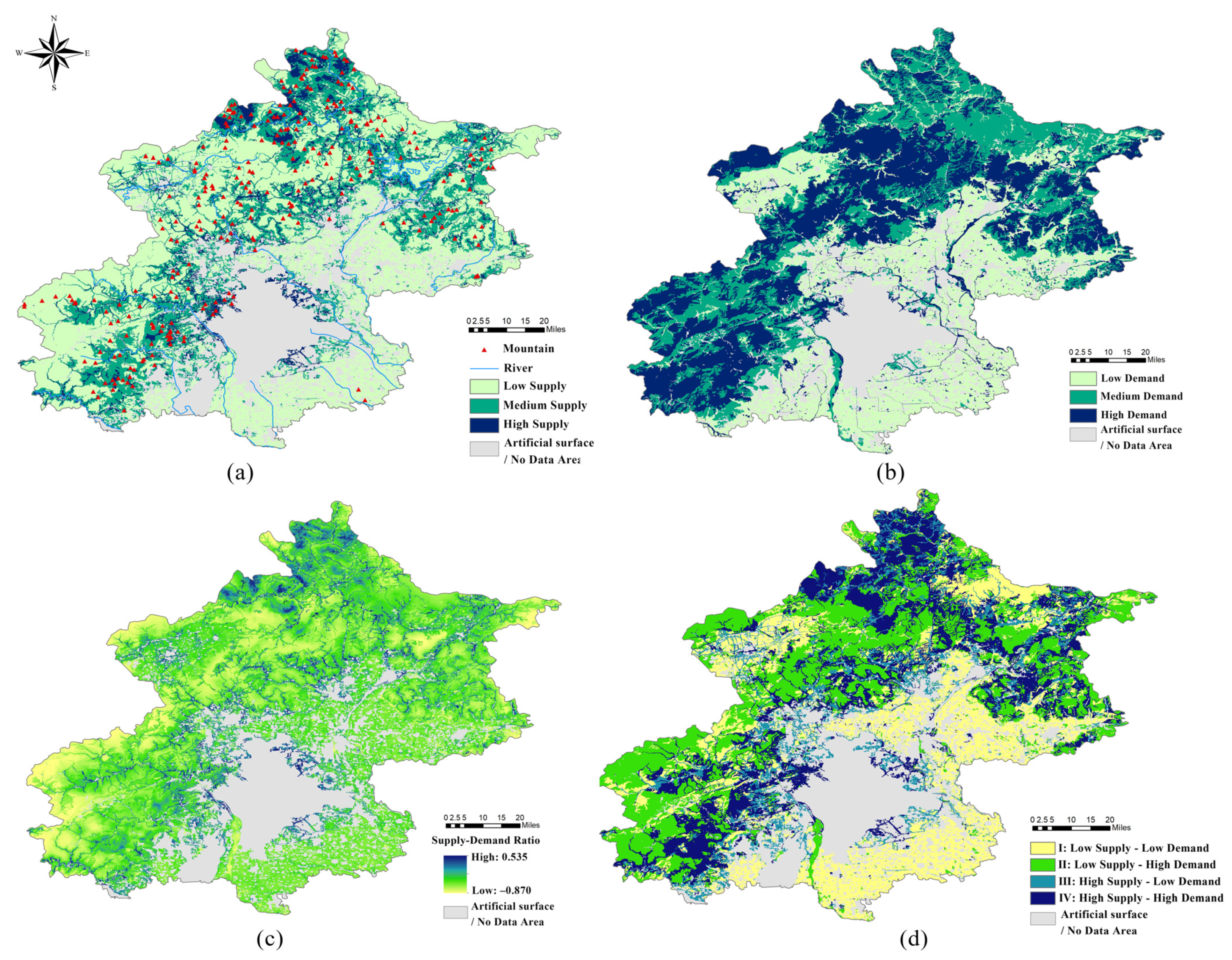
The supply of recreational services in Beijing is highly differentiated spatially (Figure 3a) due to a combination of human and natural environmental factors such as topography, ecosystem type, transportation network, and infrastructure. The area of medium and high supply only accounted for about a quarter of the total area of the study area. They were mainly distributed in the transition zone between mountainous areas and plain areas, the ecological subzone of deciduous broad-leaved forests in the northern Yanshan Mountains, and a few in the edge of the central urban areas. In terms of spatial distribution, the supply level of mountainous areas with good natural geographical conditions and intact ecological landscape is significantly higher than that of plain areas with reduced vegetation and overexploitation. The mountainous areas have a high supply in the north and a low supply in the west and southwest. The medium-supply area is mainly in the transition zone between mountainous areas and plain areas. The plain areas have low-supply areas of recreational services overall in space.

3.2. Demand for Recreational Services from Green Space

The results of descriptive statistics (

Table 5. Descriptive statistical results of the landscape types’ perceived value.

Landscape Types	Mean	Std.
Urban parks	8.029	1.914
Lakes	7.980	1.910
Wetlands	7.933	1.918
Reservoirs	7.851	2.007
Deciduous broad-leaved forests	7.812	2.208
Rivers	7.561	2.150
Paddy fields	7.506	2.168
Mixed conifer-broadleaved forests	7.476	2.317
Deciduous coniferous forests	7.394	2.279
Urban grasslands	7.327	2.160
Orchards	7.075	2.230
Montane grasslands	7.059	2.188
Villages	6.535	2.286
Shrubs	5.712	2.408
Residences	5.647	2.789
Cities	5.341	2.565
Drylands	5.190	2.434
Downtown streets	4.463	2.607
Bare rocks	4.055	2.572
Abandoned quarries	3.498	2.733
Wastelands	2.708	2.219

) showed that the highest perceived evaluation by residents was the park landscape, followed by the water landscape (represented by wetlands, lakes, etc.), and the forest landscape (represented by deciduous broad-leaved forests and mixed coniferous forests). Overall, residents had a higher evaluation of green space such as parks, forests, grasslands, and landscape containing green space elements, indicating a higher demand for recreational services in such landscape types. On the contrary, residents had a lower evaluation of non-green space landscape such as cities, streets, wastelands, etc., indicating that residents had lower demand in such landscape types.

In this study, three principal components (eigenvalues > 1) were successfully screened by using principal component analysis, and the cumulative contribution reached 61.41% (

Table 6. The results of principal component analysis.

Component	Eigenvalue	Variance (Unit: %)	Cumulative (Unit: %)
1	8.304	39.54	39.54
2	3.037	14.46	54.00
3	1.556	7.41	61.41
4	0.901	4.29	65.70
5	0.834	3.97	69.67
……
20	0.225	1.07	99.05
21	0.199	0.95	100.00

). Among them, the contribution of the first principal component (water landscape) to the total variance was 39.54%; the contribution of the second principal component (forest landscape) to the total variance was 14.46%; the contribution of the third principal component (parkland landscape) to the total variance was 7.41%. This once again verified that residents had a high demand for green space landscape types such as water bodies, forests, and parks.

The regional variation of residents’ demand for recreational services was obvious (Figure 3b). The medium- and high-demand areas were distributed in the deciduous broadleaf forest ecological zones in the southwest and northeast of Beijing and areas near rivers (Chaobai River, Yongding River, and Wenyu River, etc.). The low demand areas were concentrated in the plain areas, and a small portion was distributed in the western part of the mountainous regions (ecological zones of forest, farmland, and grassland in the intermountain basin of the upper Yongding River). The natural attributes of the green space were the main factors affecting the demand distribution.

There were large areas of natural forests and reserves concentrated in mountainous areas, with rich biodiversity, a well-functioning ecosystem, and pleasant climate conditions. Thus, residents had higher recognition of the green space and higher demand for recreational services. Forests were scattered in small parts of the plain. Agro-ecosystems accounted for the largest proportion of the plain area, but the quality of agro-ecosystems was low and could not provide satisfying recreational experiences. Therefore, the residents’ recognition of the green space landscape on the plain area was low, and the demand was also low.

3.3. Quantitative Balance and Spatial Matching of the Supply and Demand

The distribution of the supply-demand ratio was shown in Figure 3c. The gradual change from yellow to blue in the figure represented the transition from undersupply to oversupply.

In general, the quantitative balance of supply and demand in different regions varied greatly. The supply-demand ratio in most areas was negative (appearing as yellow green), indicating that recreational services in Beijing were mostly undersupplied. The balance of supply and demand in plain areas was good, mainly because the plain area is mainly agricultural area with poor recreational function and low supply, but the residents’ demand for recreational services from agricultural landscape was also low. In contrast, the balance of supply and demand in mountainous areas varies widely primarily because mountainous areas were topographically variable and species-rich, a diverse landscape pattern, and had a differential supply. Residents also have different demand for recreational services in different landscape types such as forests, wastelands and rocks.

Oversupply of recreational services was mainly located in the transition zone from plain areas to mountainous areas and northern areas. In particular, the supply-demand ratio in the northern region of Beijing was the highest because this region was an important ecological barrier of Beijing, with a lot of high-quality green space landscape and modern infrastructure providing the recreational services. The residents’ demand was relatively low, as there are abundant opportunities available to access nature.

The supply-demand ratio in the southwestern edge of Beijing was the lowest, suggesting undersupplied recreational services, primarily because the regional natural environment was severely damaged by the past mining [34] and the poor recreational infrastructure, resulting in poor innate resources for recreational services. In contrast, there is a strong demand for recreational services by the residents.

The spatial overlay function of ArcGIS 10.2 was used to create a spatial matching map (Figure 3d). The study area could be divided into region I (low supply-low demand), region II (low supply-high demand), region III (high supply-low demand), and region IV (high supply-high demand). The figure showed that the spatial matching pattern of supply and demand varied significantly. Regions II and IV were supply-demand mismatching areas, accounting for about 32 and 12% of the study area, respectively. Region I and region III were supply-demand matching areas, accounting for about 29 and 27% of the study area, respectively. The specific information of each type of region was shown in

Table 7. Spatial matching type distribution of the supply and demand.

Regions	Location	Demand Characteristics	Supply Characteristics	Causes of the Matching/Mismatching
I	The southeastern plain area and the area near the Baimaguan River wetland in the north.	Low supply	Low demand	The single type of ecosystem and high landscape homogeneity were the main reasons for the low supply-low demand pattern. In addition, the southeastern plain area is mainly construction area and agricultural area with poor recreational function and low supply. The area near the northern Baimaguang River wetland was an important water source protection area where recreational resources development was restricted. Residents also had a low demand for recreational services with a single type of green space.
II	The high mountain areas (elevation >300 m), including the southwestern edge, the north-central region.	Low supply	High demand	The green space landscape in high mountain areas had abundant and high-quality recreational resources, which greatly attracted the residents’ willingness for recreation. However, the complex topography, incomplete infrastructure, and distance from urban areas limited the supply in these areas.
III	The low mountain areas (elevation from 100 to 300 m), and the edge of the central urban areas.	High supply	Low demand	Such areas were concentrated in the vicinity of green space landscape with convenient transportation, good infrastructure, and high supply. However, the ecological damage caused by the overexploitation of recreational resources had reduced the willingness of residents to recreation.
VI	The northern mountainous areas, the edge of the low mountain areas, and the edge of the central urban areas.	High supply	High demand	The high-quality natural geographic resources and convenient infrastructure of such areas provided the conditions for supply-demand matching. The northern mountainous region had the largest area of natural forests in Beijing. The forest ecosystems of the region were intact and rich in biodiversity, providing a diverse range of landscape and ecological services. The residents had a strong demand for recreational services from green space landscape.

.

4. Discussion and Conclusions

4.1. Assessment and Mapping of Recreational Service from Green Space

The MaxEnt model was applied for the first time to assess and map the supply of recreational services from green spaces. Some studies have indicated that the MaxEnt model can provide robust results in assessing and mapping the supply of cultural/recreational services of landscapes [21,29] and farmlands [17]. Based on the MaxEnt model, this study collects POI points related to recreational services from green space and selects variables related to human and natural factors to assess and map the supply of recreational services. The AUC values of the models all exceeded 80%, again proving that the models possess good accuracy. Our research results reveal how human and natural factors affect the supply of recreational services from green space in Beijing. In general, natural factors have a dominant role in the supply of recreational services. Mountainous areas with higher peak densities, closer proximity to water bodies and accommodations have a higher recreation service supply capacity. Plain areas with high patch aggregation and patch shape complexity closer to city centers have a higher supply of recreational services. The application of the MaxEnt model also faces some limitations. For example, POI data are usually provided by map service platforms, and the completeness of POI data is limited due to platform limitations and untimely updates [35]; the selection of human and natural factors is mostly subjective, and their scientific validity needs more studies to confirm [17,25]. Since the MaxEnt model obtains robust results even for small samples [20], it is clear the selection of relevant factors is more restrictive for this method to be applied.

Understanding which landscapes are more socially preferred has important implications for urban ecosystem resource management [36]. Questionnaires or interviews are commonly used in current cultural ecosystem service needs assessments [37,38]. The selection and evaluation of recreational environments are mainly based on aesthetics and naturalness [39,40]. Visual surveys allow respondents to visualize the aesthetics and naturalness of different landscapes [36,41]. Therefore, this study uses a visual survey method to design a questionnaire to obtain the residents’ demand for recreational services from green space. The study found that residents have a higher demand for recreational services in green space landscapes (forests, grasslands, wetlands, etc.), but a lower demand for recreational services in non-green space landscapes (streets, wastelands, bare rocks, etc.). Existing studies have also found that watershed wetlands and forests are important determinants of recreational value [42], and the biodiversity and naturalness of green spaces have been found to make an important contribution to improving the health of residents and building good social relations [43,44].

4.2. Demand and Supply of Recreational Services in Plain Areas and Mountainous Areas

The MaxEnt results show that the distribution of the supply of recreational services in Beijing varies greatly due to the comprehensive influence of natural (terrains, ecosystem types, etc.) and human (transportation network, infrastructures, etc.) factors. The area of medium and high supply only accounted for about a quarter of the total area of the study area. The supply level of mountainous areas with good natural geographical conditions and intact ecological landscape is significantly higher than that of plain areas with reduced vegetation and overexploitation. The plain areas were the main distribution area of the low-supply area of recreation services. In mountainous areas, high-supply areas were concentrated in the north; low-supply areas were concentrated in the west and southwest; medium-supply areas were mainly located in the transition zone between mountainous areas and plain areas. The western and southwestern mountainous areas of Beijing are distributed with important ecological reserves; where construction and development are restricted, the supply capacity is low. The northern mountainous region of Beijing has a lot of high-quality green space landscapes (Trumpet Ditch Primitive Forest Park, Qifeng Mountain National Forest Park, etc.) and modern infrastructure, which provided a high supply of recreation services.

It is worth noting that the supply estimated by the MaxEnt model is inclusive of potential supply [21], which reflects the landscape recreation potential. The recreation potential differs from the realized service, which directly contributes to human well-being through the actual capture of the recreational services [45]. In practice, mountainous areas with good physical geography and complete ecosystem services are often distributed with important ecological reserves and national forest parks. These places have a strong recreational appeal to residents. However, the development of recreational potential in mountainous areas should be treated with caution. The increased ecological pressure caused by tourism development often leads to ecological degradation, which is particularly common in mountainous areas [46]. Trampling by tourists may lead to vegetation degradation and soil exposure in mountainous areas, combined with erosion by flowing water, may easily lead to washout and slope degradation [47].

Using ArcGIS 10.2 to overlay the standardized supply and demand data spatially to get the supply-demand spatial matching map. The results show that the supply-demand quantitative balance pattern in different regions varied greatly, and most areas show the state of undersupply. The supply-demand spatial matching pattern in different regions varied significantly too, and a certain spatial mismatch was found. There are four different types, including two spatial matching types of “low supply-low demand” and “high supply-high demand”, and two spatial mismatching types of “low supply-high demand” and “high supply-low demand”, with the area of the spatial mismatching type accounting for about half of the study area.

4.3. Suggestions

In future green space planning and management in Beijing, different development strategies such as ecological reshaping, ecological development, restoration, and protection should be implemented in different areas. It is becoming more important to improve the well-being of the residents and develop a livable city that promotes sustainable development.

In Region I (low-supply and low-demand), ecological reshaping measures should be taken to improve land use patterns and increase the area of urban green space such as forests and grasslands. This will enhance the integrity of urban ecosystems and improve the supply of recreational services. In the plain afforestation project, the preservation of planted forests should be strengthened to provide more green space that can meet the residents’ demand for recreational services. In the process of agricultural development in plain areas, attention should be paid to enhancing the recreational service function of farmland. The farmland landscape should be optimized by improving vegetation diversity and increasing recreational service facilities.

In Region II (low supply and high demand), ecological development is the top priority. The green space in such areas should be moderately developed under the premise of adhering to the ecological red line, to enhance the supply ability of recreation services and ecological carrying capacity. The high mountain areas are an important urban environmental protection barrier, with many ecological protection areas distributed. The construction and development of the area are strictly limited, and the incomplete infrastructure construction is the main factor limiting the recreation supply resources. On the premise of ensuring that the area of the ecological reserve will not be reduced and the ecological function will not be lowered, the road traffic and infrastructure construction should be optimized moderately to enhance the ecological supply capacity and ecological carrying capacity.

In Region III (high supply and low demand), it is important to implement ecological restoration. The ecological damage caused by economic construction reduces the demand for recreational services of residents. The spread of urbanization from plain areas to mountainous areas should be controlled to promote the matching of supply and demand. As a transitional zone between plains and mountains, the early economic development of low mountain areas has made the overall ecosystem fragile. Although green space is restored in the artificial afforestation project, the overall ecological landscape quality is poor, resulting in low demand for recreational services of residents. The area should expand the area of green space, enhance ecosystem integrity, improve landscape continuity, and increase landscape heterogeneity to provide a quality recreation experience.

In region IV (high supply and high demand), ecological conservation should be given top priority. Only under the principle of “conservation-oriented and rational development” can this region achieve coordinated ecological and economic development. It is necessary to coordinate all kinds of elements in the system of mountains-rivers-forests-farmlands-lakes-grasslands, and realize the diversified combination of different recreation supply subjects, to improve biodiversity and promote the stability of the ecosystem. The region should focus on improving the quality of recreational life of residents and enhancing the value of various natural ecological landscapes to better meet the recreational needs of residents.

4.4. Limitations and Future Research

This study conducted a preliminary analysis and discussion on the supply and demand situation of recreational services from green space in Beijing. Our research results are still relatively crude. This study has not considered possible temporal dynamic differences in the supply and demand, such as the impact of seasonal changes on human activities and natural landscape. Therefore, future research should incorporate spatial and temporal variables into the analysis of the supply and demand of recreational services through research design and variable selection. Moreover, the study sample will be further expanded, making the results more representative and convincing.

References

- Bertram, C.; Rehdanz, K. The role of urban green space for human well-being. Ecol. Econ. 2015, 120, 139–152. [Google Scholar] [CrossRef] [Green Version]
- Viniece, J.; Lincoln, L.; Jessica, Y. Advancing Sustainability through Urban Green Space: Cultural Ecosystem Services, Equity, and Social Determinants of Health. Int. J. Environ. Res. Public Health 2016, 13, 196. [Google Scholar]
- Millennium Ecosystem Assessment. Ecosystems and Human Well-Being: Synthesis; Island Press: Washington, DC, USA, 2005. [Google Scholar]
- Fish, R.; Church, A.; Winter, M. Conceptualising Cultural Ecosystem Services: A Novel Framework for Research and Critical Engagement. Ecosyst. Serv. 2016, 21, 208–217. [Google Scholar] [CrossRef] [Green Version]
- Tenerelli, P.; Demšar, U.; Luque, S. Crowdsourcing indicators for cultural ecosystem services: A geographically weighted approach for mountain landscapes. Ecol. Indic. 2016, 64, 237–248. [Google Scholar] [CrossRef] [Green Version]
- He, S.Y.; Su, Y.; Wang, L.; Cheng, H.G. Realisation of recreation in national parks: A perspective of ecosystem services demand and willingness to pay of tourists in Wuyishan Pilot. J. Nat. Resour. 2019, 34, 40–53. (In Chinese) [Google Scholar] [CrossRef]
- Li, F. Assessment on Recreational Services of Wetland in Beijing and Its Balance on Supply and Demand; University of Chinese Academy of Sciences: Beijing, China, 2011. (In Chinese) [Google Scholar]
- Wu, X.; Zhou, Z.X. Spatial relationship between supply and demand of ecosystem services through urban green infrastructure: Case of Xi’an City. Acta Ecol. Sin. 2019, 39, 9211–9221. (In Chinese) [Google Scholar]
- Depietri, Y.; Kallis, G.; Baró, F.; Cattaneo, C. The urban political ecology of ecosystem services: The case of Barcelona. Ecol. Econ. 2016, 125, 83–100. [Google Scholar] [CrossRef]
- Heynen, N. Urban Political Ecology III: The Feminist and Queer Century. Prog. Hum. Geogr. 2018, 42, 446–452. [Google Scholar] [CrossRef] [Green Version]
- Heynen, N. Urban Political Ecology II: The Abolitionist Century. Prog. Hum. Geogr. 2016, 40, 839–845. [Google Scholar] [CrossRef]
- Heynen, N. Urban Political Ecology I: The Urban Century. Prog. Hum. Geogr. 2014, 38, 598–604. [Google Scholar] [CrossRef]
- Kull, C.A.; Sartre, X.A.D.; Castro-Larrañaga, M. The political ecology of ecosystem services. Geoforum 2015, 61, 122–134. [Google Scholar] [CrossRef] [Green Version]
- Ma, L.; Liu, H.; Peng, J.; Wu, J.S. A review of ecosystem services supply and demand. Acta Geogr. Sin. 2017, 72, 1277–1289. (In Chinese) [Google Scholar]
- Burkhard, B.; Kroll, F.; Nedkov, S.; Müller, F. Mapping ecosystem service supply, demand and budgets. Ecol. Indic. 2012, 21, 17–29. [Google Scholar] [CrossRef]
- Baró, F.; Palomo, I.; Zulian, G.; Vizcaino, P.; Haase, D.; Gómez-Baggethun, E. Mapping ecosystem service capacity, flow and demand for landscape and urban planning: A case study in the Barcelona metropolitan region. Land Use Policy 2016, 57, 405–417. [Google Scholar] [CrossRef] [Green Version]
- He, S.; Su, Y.; Shahtahmassebi, A.R.; Huang, L.Y.; Zhou, M.M.; Gan, M.Y.; Deng, J.S.; Zhao, G.; Wang, K. Assessing and mapping cultural ecosystem services supply, demand and flow of farmlands in the Hangzhou metropolitan area, China. Sci. Total Environ. 2019, 692, 756–768. [Google Scholar] [CrossRef]
- Elith, J.; Graham, C.H.; Anderson, R.P.; Dudík, M.; Ferrier, S.; Guisan, A.; Hijmans, R.J.; Huettmann, F.; Leathwick, J.R.; Lehmann, A.; et al. Novel methods improve prediction of species’ distributions from occurrence data. Ecography 2006, 29, 129–151. [Google Scholar] [CrossRef] [Green Version]
- Phillips, S.J.; Anderson, R.P.; Schapire, R.E. Maximum entropy modeling of species geographic distributions. Ecol. Model. 2006, 190, 231–259. [Google Scholar] [CrossRef] [Green Version]
- Wisz, M.S.; Hijmans, R.J.; Li, J.; Peterson, A.T.; Graham, C.H.; Guisan, A. Effects of sample size on the performance of species distribution models. Divers. Distrib. 2008, 14, 763–773. [Google Scholar] [CrossRef]
- Yoshimura, N.; Hiura, T. Demand and supply of cultural ecosystem services: Use of geotagged photos to map the aesthetic value of landscapes in Hokkaido. Ecosyst. Serv. 2017, 24, 68–78. [Google Scholar] [CrossRef]
- Wang, Y.S.; Xie, B.Y.; Wan, F.H.; Xiao, Q.M.; Dai, L.Y. Application of ROC curve analysis in evaluating the performance of alien species’ potential distribution models. Biodivers. Sci. 2007, 15, 365–372. (In Chinese) [Google Scholar]
- Guo, J.; Liu, X.P.; Zhang, Q.; Zhang, D.F.; Xie, C.X.; Liu, X. Prediction for the potential distribution area of Codonopsis pilosula at global scale based on Maxent model. Chin. J. Appl. Ecol. 2017, 28, 992–1000. (In Chinese) [Google Scholar]
- Richards, D.R.; Tunçer, B. Using image recognition to automate assessment of cultural ecosystem services from social media photographs. Ecosyst. Serv. 2018, 31, 318–325. [Google Scholar] [CrossRef]
- Schirpke, U.; Meisch, C.; Marsoner, T.; Tappeiner, U. Revealing spatial and temporal patterns of outdoor recreation in the European Alps and their surroundings. Ecosyst. Serv. 2018, 31, 336–350. [Google Scholar] [CrossRef]
- Casado-Arzuaga, I.; Onaindia, M.; Madariaga, I.; Verburg, P.H. Mapping recreation and aesthetic value of ecosystems in the Bilbao Metropolitan Greenbelt (northern Spain) to support landscape planning. Landsc. Ecol. 2013, 29, 1393–1405. [Google Scholar] [CrossRef]
- Li, X.; Zhu, D.; Lin, P. Dynamic analysis of landscape and quality assessment of cultivated land use in piedmont belt. China Land Sci. 2000, 14, 40–42. (In Chinese) [Google Scholar]
- Li, W.B.; Wang, D.Y.; Li, H.; Liu, S.H. Urbanization-induced site condition changes of peri-urban cultivated land in the black soil region of northeast China. Ecol. Indic. 2017, 80, 215–223. [Google Scholar] [CrossRef]
- Clemente, P.; Calvache, M.; Antunes, P.; Santos, R.; Cerdeira, J.O.; Martins, M.J. Combining social media photographs and species distribution models to map cultural ecosystem services: The case of a Natural Park in Portugal. Ecol. Indic. 2019, 96, 59–68. [Google Scholar] [CrossRef]
- Richards, D.R.; Friess, D.A. A rapid indicator of cultural ecosystem service usage at a fine spatial scale: Content analysis of social media photographs. Ecol. Indic. 2015, 53, 187–195. [Google Scholar] [CrossRef]
- Sheppard, S.R.J. Visual Simulation: A User’s Guide for Architect, Engineers, and Planners; Van Nostrand Reinhold Company Inc.: New York, NY, USA, 1989. [Google Scholar]
- Li, J.H.; Jiang, H.W.; Bai, Y.; Alatalo, J.M.; Li, X.; Jiang, H.W.; Liu, G.; Xu, J. Indicators for spatial-temporal comparisons of ecosystem service status between regions: A case study of the Taihu River Basin, China. Ecol. Indic. 2016, 60, 1008–1016. [Google Scholar] [CrossRef]
- Li, Y.; Zhang, X.W.; Fang, Y.M. Responses of the distribution pattern of Quercus chenii to climate change following the Last Glacial Maximum. Chin. J. Plant Ecol. 2016, 40, 1164–1178. (In Chinese) [Google Scholar]
- Wang, J.; Cheng, W.M.; Qi, S.L.; Zhou, C.H.; Zhang, W.J.; Tong, C.M. Sensitive evaluation and spatial analysis of soil and water loss based on USLE and GIS: Taking Taihang Mountain area of Hebei Province as an example. Geogr. Res. 2014, 33, 614–624. [Google Scholar]
- Zhang, X.; Du, S.; Wang, Q. Hierarchical semantic cognition for urban functional zones with VHR satellite images and POI data. Isprs. J. Photogramm. Remote Sens. 2017, 132, 170–184. [Google Scholar] [CrossRef]
- Peña, L.; Casado-Arzuaga, I.; Onaindia, M. Mapping recreation supply and demand using an ecological and a social evaluation approach. Ecosyst. Serv. 2015, 13, 108–118. [Google Scholar] [CrossRef]
- Cabana, D.; Ryfield, F.; Crowe, T.P.; Brannigan, J. Evaluating and communicating cultural ecosystem services. Ecosyst. Serv. 2020, 42, 101085. [Google Scholar] [CrossRef]
- Kaltenborn, B.P.; Linnell, J.D.C.; Gómez-Baggethun, E. Can cultural ecosystem services contribute to satisfying basic human needs? A case study from the Lofoten archipelago, northern Norway. Appl. Geogr. 2020, 120, 102229. [Google Scholar] [CrossRef]
- Goodness, J.; Andersson, E.; Anderson, P.M.L.; Elmqvist, T. Exploring the links between functional traits and cultural ecosystem services to enhance urban ecosystem management. Ecol. Indic. 2016, 70, 597–605. [Google Scholar] [CrossRef]
- Daniel, T.C.; Muhar, A.; Arnberger, A.; Aznar, O.; Boyd, J.W.; Chan, K.M.A.; Costanza, R.; Elmqvist, T.; Flint, C.G.; Gobster, P.H.; et al. Contributions of cultural services to the ecosystem services agenda. Proc. Natl. Acad. Sci. USA 2012, 109, 8812–8819. [Google Scholar] [CrossRef] [PubMed] [Green Version]
- Maes, J.; Paracchini, M.L.; Zulian, G.; Dunbar, M.B.; Alkemade, R. Synergies and trade-offs between ecosystem service supply, biodiversity, and habitat conservation status in Europe. Biol. Conserv. 2012, 155, 1–12. [Google Scholar] [CrossRef]
- Voigt, A.; Kabisch, N.; Wurster, D.; Haase, D.; Breuste, J. Structural Diversity: A Multi-dimensional Approach to Assess Recreational Services in Urban Parks. AMBIO A J. Hum. Environ. 2014, 43, 480–491. [Google Scholar] [CrossRef] [Green Version]
- Barrantes-Sotela, O. Aportes desde la conservación genética al mejoramiento de las áreas verdes en la ciudad Contributions from genetic conservation to the improvement of urban green spaces. Rev. Geogr. Am. Cent. 2020, 1, 43–57. [Google Scholar]
- Mireia, G.; Margarita, T.M.; David, M.; Payam, D.; Joan, F.; Antoni, P.; Mark, N. Mental Health Benefits of Long-Term Exposure to Residential Green and Blue Spaces: A Systematic Review. Int. J. Environ. Res. Public Health 2015, 12, 4354–4579. [Google Scholar]
- Weyland, F.; Laterra, P. Recreation potential assessment at large spatial scales: A method based in the ecosystem services approach and landscape metrics. Ecol. Indic. 2014, 39, 34–43. [Google Scholar] [CrossRef]
- Geneletti, D.; Dawa, D. Environmental impact assessment of mountain tourism in developing regions: A study in Ladakh, Indian Himalaya. Environ. Impact Assess. Rev. 2009, 29, 229–242. [Google Scholar] [CrossRef]
- Dudek, T. Recreational potential as an indicator of accessibility control in protected mountain forest areas. J. Mt. Sci. 2017, 14, 187–195. [Google Scholar] [CrossRef]
Figure 1.
The administrative divisions map (a) and DEM (b) of Beijing.
Figure 2.
ROC curve verification of MaxEnt prediction in mountainous areas (a) and plain areas (b).
Figure 3.
The supply distribution (a), demand distribution (b), supply-demand ratio distribution, (c) and spatial matching map (d) of recreational services from green space in Beijing.