The Concept and Understanding of Synchronous Stability in Power Electronic-Based Power Systems

Abstract

Synchronous stability in power systems is of essential importance for system safety and operation. For the phase-locked loop (PLL)-based synchronous stability in power electronic-based power systems, which has recently stimulated interest in researchers in the field of electrical power engineering, but is still controversial, this paper divides the topic into two aspects, including the PLL device stability and the system stability. It is found that the PLL device is always stable and the error between the PLL output angle ${\theta }_{pll}$ and the terminal voltage angle ${\theta }_t$ is always finite. Therefore, the synchronization of power electronic-based power systems should be understood as the output synchronization between the electrical rotation vectors (${\theta }_t$ or ${\theta }_{pll}$) from each item of grid-tied equipment, rather than the synchronization of the PLL device itself. In addition, it is found that ${\theta }_{pll}$ plays an active role in the system synchronization dynamics not only in electromagnetic timescales but also electromechanical timescales and it could be selected as a dominant observable. In this paper, the concept of synchronous stability is well clarified. These findings are well supported by theoretical analyses and MATLAB/Simulink simulations, and thus could provide insights on the synchronous stability mechanism.

1. Introduction

With the increase in electricity demand and global targets for carbon neutrality, it becomes necessary to accelerate the construction of power electronic-based power systems (or renewable-dominated new-type power systems) [1]. In recent years, a large number of renewable equipment, including doubly fed induction generators, permanent magnet synchronous generators (PMSGs), and photovoltaics, have been connected to the power grid through power electronic inverters. Most of them are voltage source converters (VSCs) by using the mature technique of phase-locked loop (PLL) [2]. Accordingly, the power system dynamic performance has been greatly changed due to these new devices. This also alters all aspects of power systems, including analysis, relaying, control, and operation. Until now, we, human beings, have not yet fully utilized them [1,2].

As the alternating current transmission technique is still unchanged, it is quite natural to see that the synchronous stability, which is also called rotor-angle stability in the traditional power systems, plays a similar, important role in the system integrity and stability [3,4]. Indeed, the transient synchronous stability of power electronic-based power systems under large disturbances has become a very hot topic recently [5,6]. Most previous studies focused on the simple model of a PLL-based VSC single-machine infinite-bus system, and usually considered only one PLL controller in the system [7,8,9,10,11,12,13,14]. Various methods, including the time-domain simulation, phase portrait, energy function (or Lyapunov function), equal area criterion, bifurcation analysis, etc., have been borrowed and developed [11,12,13,14]. In addition, a variety of transient synchronous stability enhancement methods have also been proposed [14,15,16]. Very recently there have been some advancements by considering outer controller effects [17,18] and multiple-VSC systems [19]. At the same time, the impact of virtual inertia control on the dynamic system behavior has attracted the attention of researchers, and it has been found that it not only efficiently supports the system frequency but also affects the synchronous stability characteristics [20,21].

Although the synchronous stability in power electronic-based power systems has been widely studied in electric power engineering, there are still several key problems remaining to be answered. On the one hand, usually the model is very restricted to the simple model of a PLL-based VSC single-machine infinite-bus system with all outer controllers ignored. The objective is to simply concentrate on the PLL effect in synchronization. It is far away from realistic large-scale systems in engineering. So far, it seems that only synchronous stability within the electromagnetic timescale has been reported. On the other hand, for the concept and understanding of the synchronous stability, some phrases, e.g., “the PLL instability issues” [9], “the PLL fails to track the main grid fundamental frequency” [7], “incapability of PLL to remain synchronized to the grid” [22], “instability of PLL to accurately track the phase angle of the voltage” [23,24], “instability in PLLs of grid-following inverters in weak grids” [25], etc., have been scattered throughout the literature, making the concept of synchronous stability obscure. It is unclear whether the synchronous stability is either the PLL device stability (between the PLL input and output) or system stability (between the grid-tied devices). Additionally, until now, the system dominant variable in the synchronous stability has been unclear [26].

Faced with these interesting, unsolved, basic problems, this paper attempts to clarify the key concept of synchronous stability in power electronic-based power systems. The remainder of this paper is structured as follows. Section 2 gives the structural decomposition of power electronic-based power systems. In Section 3, the stability and dynamic response of PLL controller are analyzed by linearization. In Section 4, the stability of PLL-based VSC system is analyzed from three aspects: the steady-state stability, small-signal stability, and large-signal stability. In Section 5, the effectiveness of the theoretical analysis is verified and supplemented by MATLAB/Simulink simulation. Section 6 gives our understanding of the concept of synchronous stability. Finally, our conclusions and discussions are given in Section 7.

2. Structural Decomposition of Power Electronic-Based Power Systems

At present, three are three typical types of renewable energy device connected to the power grid, including the PMSGs and doubly fed induction generators for the wind power, and photovoltaics for the solar power. Although there are some differences in their control structures, all of them use the PLL technique to realize synchronization with the grid. Their synchronization mechanism is similar. Therefore, in this paper we will take the PMSG single-machine infinite-bus system as an example, to clarify the concept of synchronous stability in power electronic-based power systems, without losing generality.

2.1. PMSG Single-Machine Infinite-Bus System

Figure 1 shows the topology of the PMSG single-machine infinite-bus system, including both the machine-side (left) and grid-side (right) controllers, which are separated completely, but connected by a DC-link capacitor C in the middle of the figure. On the left, the machine-side converter (MSC) adopts the zero d axis current control, including the rotor speed control (RSC), the alternating current control (ACC), and the additional inertia control (AIC). The q axis current reference $i_{sqref}$ of the stator is given by the outputs of the RSC and AIC, and the d axis current reference $i_{sdref}$ of the stator is set to 0. According to the current references, the ACC generates the modulation voltages $e_{sd}$ and $e_{sq}$. After the coordinate transformation of the $dq$ reference frame to the $abc$ reference frame, the trigger signals are generated by the pulse width modulation (PWM). To be simple, for the slower electromechanical controls, the pitch angle control and the maximum power point tracking control of the PMSG are ignored. On the right of Figure 1, the grid-side converter (GSC) is connected to the infinite-bus (with a constant voltage amplitude $U_g$ and a constant frequency ${\omega }_g$) through the filter inductance $L_f$ and line inductance $L_g$. The control part of the GSC is divided into the DC-link voltage control (DVC), the terminal voltage control (TVC), the ACC, and the PLL. The DVC gives the d axis current reference $i_{dref}$ by controlling the capacitor voltage $U_{dc}$, and the TVC gives the q axis current reference $i_{qref}$ by controlling the terminal voltage $U_t$. According to the current references, the ACC generates the modulation voltages $e_d$ and $e_q$. After the coordinate transformation of the $dq$ reference frame to the $abc$ reference frame, the trigger signals are also generated by the PWM. Here, $e_{abc}$ and $u_{tabc}$ are used to denote the VSC arm output voltage and the VSC terminal voltage, respectively. $e_{abc}$ is also widely termed as the internal potential in the literature. In the grid connection control, the PLL technique is crucial, as it provides the $dq$-reference frame for the control of the GSC and makes the grid-tied synchronization possible.

2.2. PLL-Based VSC Single-Machine Infinite-Bus System

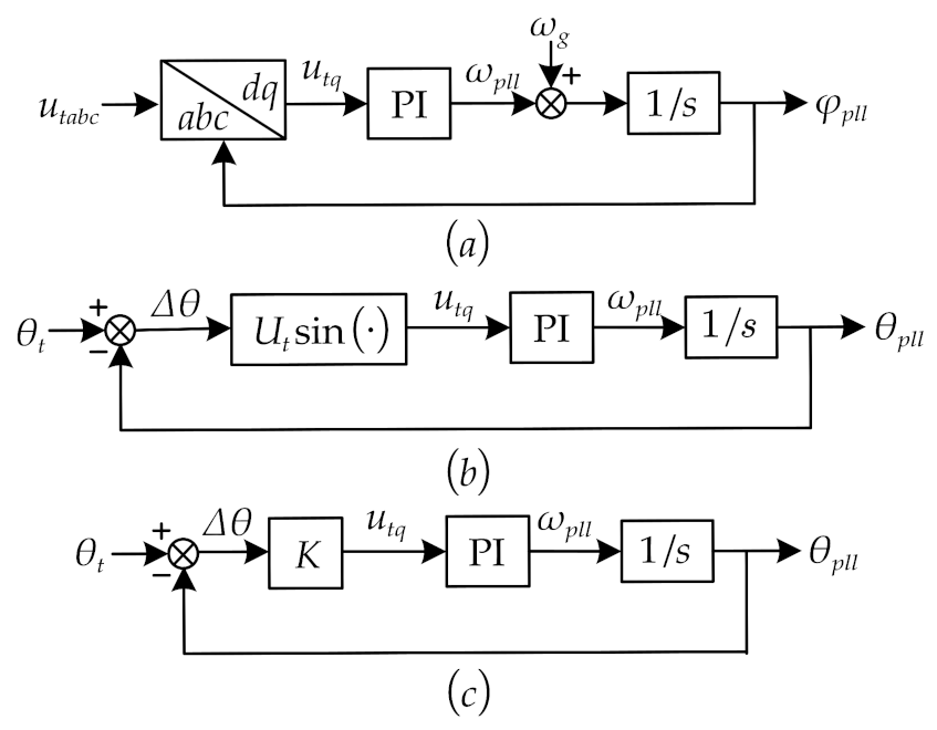
In the absence of inertia control, the PMSG simply outputs power from the MSC to GSC, and then to the grid, by the DC-link capacitor, and the MSC does not respond any faults from the grid. The MSC and GSC are separated. Hence, it is quite natural to consider the GSC dynamics only. In this respect, the whole system can be simplified into a PLL-based VSC single-machine infinite-bus system, as illustrated by the large dashed-line frame in Figure 1. Hence, $P_m=constant$. Nevertheless, if the inertia control is incorporated, this dynamical separation might be unavailable and both MSC and GSC should be considered together. In addition, as the PLL dynamics is much slower than that of the ACC, it is usually assumed that the output currents instantaneously track their references, namely, $i_d=i_{dref}$ and $i_q=i_{qref}$ [17]. Under these simplifications, the VSC can be treated as a controlled current source, and the whole system is schematically shown in Figure 2a.

Next, if all outer controllers including the usual DVC and TVC are ignored, only the PLL dynamics should be studied. This is possible, under some certain situations, such as low voltage ride through, where all current commands are fixed ($i_{dref}=constant$ and $i_{qref}=constant$) [11]. The corresponding simplified system is schematically shown in Figure 2b. Note that this model has been widely studied in the synchronous stability research, due to its simplicity and importance [5,6,7,8,9,10,11,12,13,14].

2.3. PLL Controller

The PLL controller is also a closed-loop control system which tracks the phase of the input signal. Taking a close look at the PLL, it is composed of the phase detector (PD), the loop filter (LF), and the voltage-controlled oscillator (VCO). The second-order synchronous-reference-frame phase-locked loop (SRF-PLL) has been widely used in academic research and engineering applications [27,28]. Unless otherwise specified, the PLL in the paper refers to the SRF-PLL. The control structure is shown in Figure 3a. To be simpler, it can be converted into the phase model within the $xy$ common reference frame, as shown in Figure 3b. In addition, Figure 3c shows the linearized phase model of the PLL.

To be clear, Figure 4 shows the coordinate relations between the $abc$ stationary reference frame, the $dq$ rotating reference frame, and the $xy$ common reference frame, and the associated angles. The control goal of the PLL is to make the terminal voltage $U_t$ on the d axis, namely $u_{tq}=0$, $u_{td}=U_t$, or ${\theta }_{pll}={\theta }_t$.

2.4. Hierarchical Structure and Their Connections

So far, focusing on the synchronous stability problem, this paper has divided the original system into three different levels from macroscopic to microscopic views, namely, the levels of the PMSG single-machine infinite-bus system (Level I), the PLL-based VSC single-machine infinite-bus system (Level II), and the PLL controller (Level III). All three levels exhibit a clear hierarchical structure. Only if the inner level is stable can the outer level be stable. Otherwise, the system will be unstable. Basically, from a power system point of view, levels I and II have system-level stability problems, whereas level III has only a device-level stability problem. Level II has been adequately studied in the literature [5,6,7,8,9,10,11,12,13,14].

The most inner level III of the PLL device may have a stability problem as it is also a closed-loop system. In particular, this paper is interested in whether the PLL output angle ${\theta }_{pll}$ can always track the terminal voltage angle ${\theta }_t$, or, if not, can this loss of synchronization further induce system-level instability on level II. Comparing levels II in Figure 2b and III in Figure 3, it is found that they are similar and both are second-order dynamical systems. However, level III is determined by the input signal ${\theta }_t$, whereas level II is not. With the standard language of dynamical systems, level III for the PLL device is a non-autonomous system, and level II for the PLL-based VSC system is an autonomous one. Moreover, this paper is interested in the synchronous stability of level I and its relation with that of level II, which are seldom studied.

3. Stability and Response Analyses of PLL Controller

3.1. Small-Signal Stability Analysis

This section deals with the PLL device in Figure 3. When the PLL is in a synchronous state, the transient error $\Delta \theta$ ($\Delta \theta ={\theta }_t-{\theta }_{pll}$) is tiny (close to zero) and the PD can be considered as linear. Therefore, a line with slope K can be used to approximate the characteristics of the PD. The system can be linearized and simplified with its control block diagram presented in Figure 3c; $K=U_t$. Under this situation, the closed-loop transfer function of the PLL (with ${\theta }_t$ as input and ${\theta }_{pll}$ as output) can be obtained as follows:

$$G\left(s\right)=\frac{{\theta }_{pll}\left(s\right)}{{\theta }_t\left(s\right)}=\frac{K{k}_{p,pll}s+K{k}_{i,pll}}{s^2+K{k}_{p,pll}s+K{k}_{i,pll}},$$

(1)

which can be further expressed in the standard form as

$$G\left(s\right)=\frac{2\xi {\omega }_{n}s+{\omega }_n^2}{s^2+2\xi {\omega }_{n}s+{\omega }_n^2},$$

(2)

where ${\omega }_n=\sqrt{K{k}_{i,pll}}$ and $\xi =\frac{K{k}_{p,pll}}{2\sqrt{K{k}_{i,pll}}}$ denote the natural frequency and the damping ratio, respectively.

Based on the facts that the system small-signal stability is determined by the characteristic equation: $s^2+2\xi {\omega }_{n}s+{\omega }_n^2$, and the controller parameters are always greater than zero, $k_{p,pll}>0$ and $k_{i,pll}>0$, and $K>0$, it is easy to obtain that the PLL device should always be small-signal stable.

3.2. Dynamic Response Analysis

Next, this section studies the dynamic responses of the PLL device under different disturbances ${\theta }_t$ and calculates their errors $\Delta \theta$ ($\Delta \theta ={\theta }_t-{\theta }_{pll}$). According to the control diagram in Figure 3c, the error transfer function of the PLL can be expressed as

$$G^{\prime }\left(s\right)=\frac{\Delta \theta \left(s\right)}{{\theta }_t\left(s\right)}=\frac{s^2}{s^2+2\xi {\omega }_{n}s+{\omega }_n^2}.$$

(3)

Accordingly, the steady-state errors under three typical input signals can be analyzed as follows.

1.

When the input signal is a phase step, i.e.,

$${\theta }_t\left(s\right)=\frac{{\theta }_0}{s},$$

(4)

where ${\theta }_0$ denotes the difference before and after the phase step. The error response in the complex-frequency domain is obtained,

$$\Delta \theta \left(s\right)=\frac{s{\theta }_0}{s^2+2\xi {\omega }_{n}s+{\omega }_n^2},$$

(5)

and the corresponding error in the time domain is

$$\Delta \theta \left(t\right)={\theta }_0{e}^{-\xi {\omega }_{n}t}\left(cos{\omega }_n\sqrt{1-{\xi }^2}t-\frac{\xi }{\sqrt{1-{\xi }^2}}sin{\omega }_n\sqrt{1-{\xi }^2}t\right).$$

(6)

Clearly when $t\to \infty$, the steady-state error vanishes.

2.

When the input signal is a frequency step, i.e.,

$${\theta }_t\left(s\right)=\frac{{\omega }_0}{s^2},$$

(7)

where ${\omega }_0$ denotes the difference before and after the frequency step. Correspondingly, the error response in the complex-frequency domain is obtained,

$$\Delta \theta \left(s\right)=\frac{{\omega }_0}{s^2+2\xi {\omega }_{n}s+{\omega }_n^2},$$

(8)

and that in the time domain is

$$\Delta \theta \left(t\right)={\omega }_0{e}^{-\xi {\omega }_{n}t}\frac{sin{\omega }_n\sqrt{1-{\xi }^2}t}{{\omega }_n\sqrt{1-{\xi }^2}}.$$

(9)

Clearly when $t\to \infty$, the steady-state error vanishes again.

3.

When the input signal is a frequency ramp, i.e.,

$${\theta }_t\left(s\right)=\frac{R_0}{s^3},$$

(10)

where $R_0$ represents the slope of the change in frequency. Correspondingly, the error response in the complex-frequency domain is

$$\Delta \theta \left(s\right)=\frac{R_0}{s\left(s^2+2\xi {\omega }_{n}s+{\omega }_n^2\right)},$$

(11)

and that in the time domain is

$$\Delta \theta \left(t\right)=\frac{R_0}{{\omega }_n^2}-\frac{R_0}{{\omega }_n^2}{e}^{-\xi {\omega }_{n}t}\left(cos{\omega }_n\sqrt{1-{\xi }^2}t+\frac{\xi }{\sqrt{1-{\xi }^2}}sin{\omega }_n\sqrt{1-{\xi }^2}t\right),$$

(12)

Under this situation, when $t\to \infty$, the steady-state error is finite and equals $\frac{R_0}{{\omega }_n^2}$.

The steady-state errors of the PLL under these three typical disturbances are summarized in

Table 1. Summary of steady-state error of the PLL device for different inputs ${\theta }_t$.

	Phase Step	Frequency Step	Frequency Ramp
$\Delta \theta$	0	0	$\frac{R_0}{{\omega }_n^2}$

, which clearly shows that the errors are always finite for different disturbances, i.e., ${\theta }_{pll}\approx {\theta }_t$. This indicates that the PLL can always work perfectly and its output angle ${\theta }_{pll}$ can track the terminal voltage angle ${\theta }_t$ well.

Here it is necessary to address that these analytical results only give preliminary insights for the synchronous stability mechanism. In actuality, the PLL device on level III is only one component within the whole system of level I. Its output angle ${\theta }_{pll}$ is controlled by its input ${\theta }_t$, but ${\theta }_{pll}$ also provides the control reference frame and influences the VSC output, such as the internal potential or the controlled current source output, which can further influence the dynamical process of ${\theta }_t$ with the network interaction. Therefore, ${\theta }_t\to {\theta }_{pll}\to {\theta }_t$ works as a larger close-loop in this coupled system. Thus, there is no given fixed form of ${\theta }_t$, as we have provided. The result of perfect synchronization of the PLL controller should be further checked in system-level numerical simulations.

4. Stability Analyses of PLL-Based VSC System

Here, the PLL-based VSC system in Figure 2b is studied. There are three types of synchronous stability, namely, the steady-state stability, small-signal stability, and large-signal stability. These are similar to those in the traditional power systems [4]. The steady-state stability means that there is an operating point after disturbances. The existence of an operating point is essential for system operation. Under the steady-state stable condition, small-signal stability and large-signal stability should be further considered. Small-signal stability refers to the system stability under small perturbations, and the system can be dealt with linear system theory. Alternatively, the large-signal stability means that the system stability under large perturbations and the system non-linearity under different perturbations has to be considered; typically it is associated with the determination and computation of a basin of attraction for the post-fault state [17].

4.1. Steady-State Analysis

For the electromagnetic power output $P_e$ from the VSC, it satisfies

$$P_e=u_{td}{i}_d+u_{tq}{i}_q=U_t{i}_{dref},$$

(13)

based on the facts that $u_{tq}=0$, $u_{td}=U_t$, and $i_d=i_{dref}$ in the steady state.

At the same time, due to the power transmission constraints on the network, $P_e$ should be determined by

$$P_e=\frac{U_t{U}_g}{{\omega }_g{L}_g}sin{\theta }_{pll},$$

(14)

as ${\theta }_{pll}={\theta }_t$ in the steady state.

Combining (13) and (14), it can be observed that

$$i_{dref}=\frac{U_g}{{\omega }_g{L}_g}sin{\theta }_{pll},$$

(15)

and, therefore,

$$i_{dref}\le \frac{U_g}{{\omega }_g{L}_g}.$$

(16)

This clearly indicates that there is a limit for the active current output. This result is identical to that in [7].

4.2. Small-Signal Stability Analysis

The PLL-based VSC system is determined by both the PLL differential dynamic equations:

$$\left\{\begin{array}{c}{\dot{\theta }}_{pll}={\omega }_{pll}\hfill \\ {\dot{\omega }}_{pll}=k_{p,pll}{\dot{u}}_{tq}+k_{i,pll}{u}_{tq}\hfill \end{array}\right.,$$

(17)

and the algebraic equation for the relation between the terminal voltage and the infinite-bus voltage:

$$u_{tq}=-U_{g}sin{\theta }_{pll}+i_{dref}\left({\omega }_{pll}+{\omega }_g\right)L_g,$$

(18)

where the dynamic frequency effect of the transmission-line inductance is included.

Linearizing them around the operating point, we have the following state equations

$$\left[\begin{array}{c}p\Delta {\theta }_{pll}\hfill \\ p\Delta {\omega }_{pll}\hfill \end{array}\right]=\left[\begin{array}{cc}0& 1\\ \frac{-k_{i,pll}{U}_{g}cos{\theta }_{pll0}}{1-k_{p,pll}{i}_{dref}{L}_g}& \frac{k_{i,pll}{i}_{dref}{L}_g-k_{p,pll}{U}_{g}cos{\theta }_{pll0}}{1-k_{p,pll}{i}_{dref}{L}_g}\end{array}\right]\left[\begin{array}{c}\Delta {\theta }_{pll}\hfill \\ \Delta {\omega }_{pll}\hfill \end{array}\right],$$

(19)

where $cos{\theta }_{pll0}$ is a constant, depending on the state.

On the basis of linear system theory, the following small-signal stability conditions are obtained:

$$k_{p,pll}<\frac{1}{i_{dref}{L}_g}\mathrm{and}{k}_{i,pll}<\frac{U_{g}cos{\theta }_{pll0}}{i_{dref}{L}_g}{k}_{p,pll}.$$

(20)

Accordingly, Figure 5 shows the parameter distribution for its small-signal stability with the variations of $k_{p,pll}$ and $k_{i,pll}$. Compared with the whole parameter space for the small-disturbance stability of the PLL device, here the parameter choice becomes much restricted.

4.3. Large-Signal Stability Analysis

In the above analysis, substituting the algebraic Equation (18) into the differential Equation (17), the following non-linear differential equation for the PLL-based VSC system can be obtained:

$$M{\ddot{\theta }}_{pll}=P_m-P_e+D{\dot{\theta }}_{pll},$$

(21)

where

$$\left\{\begin{array}{c}M=1-k_{p,pll}{i}_{dref}{L}_g\hfill \\ P_m=k_{i,pll}{\omega }_g{i}_{dref}{L}_g\hfill \\ P_e=k_{i,pll}{U}_{g}sin{\theta }_{pll}\hfill \\ D=k_{i,pll}{i}_{dref}{L}_g-k_{p,pll}{U}_{g}cos{\theta }_{pll}\hfill \end{array}\right..$$

(22)

Here, M, $P_m$, $P_e$, and D denote the equivalent inertia, equivalent input electromechanical power, equivalent output electromagnetic power, and equivalent damping coefficient, respectively. Clearly it is similar to the second-order swing equation of the SG; hence, it has been termed as the generalized swing equation [11], to emphasize its centrality in the synchronous stability problem. It has also been found that the basin boundary of the stable equilibrium point can show either a close-loop or a fish-like pattern, depending on different system parameters [11]. In addition, this equation has been extensively and intensively studied by different theoretical methods, such as the classical equal area criterion (EAC), energy function method, La Salle’s invariance principle, etc. [11,13,29]. The EAC judges the system stability by analyzing the acceleration and deceleration area of the system before and after faults. The energy function method gives the strict stability criterion of the system by constructing a Lyapunov function. The La Salle’s invariance principle is the extension of the Lyapunov’s second method, with the aim to find the stable boundary of system. All of them are difficult to analyze the stability of higher-order systems.

5. Simulation Results

In order to validate the above theoretic analyses, broad simulations with MATLAB/Simulink have been performed, based on the models of the PLL-based VSC system in Figure 2 and the PMSG system in Figure 1. Some results are presented below.

5.1. PLL-Based VSC Single-Machine Infinite-Bus System

To be generic, the voltage outer loop controllers are included, as shown in Figure 2a. All detailed parameters are given in Appendix A. Two cases are listed as follows:

• Case I: set the fault as the voltage $U_g$ dips 0.2 p.u. at $t=0.1$ s;
• Case II: set the fault as the voltage $U_g$ dips 0.4 p.u. at $t=0.1$ s.

The simulation results of ${\theta }_t$ and ${\theta }_{pll}$ for Case I are shown in Figure 6a, where the system is stable after a short transient process, whereas for Case II in Figure 6b, the system becomes unstable and both ${\theta }_t$ and ${\theta }_{pll}$ go to infinity. To be clearer, Figure 6c,d exhibits the phase difference $\Delta \theta$ between ${\theta }_{pll}$ and ${\theta }_t$ for these two cases. Obviously ${\theta }_t\approx {\theta }_{pll}$ in the whole dynamic process, i.e., ${\theta }_{pll}$ always tracks ${\theta }_t$ well.

Compared with the large divergence of both ${\theta }_{pll}$ and ${\theta }_t$ to infinity in Figure 6b, the mismatch between ${\theta }_{pll}$ and ${\theta }_t$ in Figure 6d is tiny and ignorable. Therefore, the PLL device does not show any inherent desynchronization between ${\theta }_{pll}$ and ${\theta }_t$. This is consistent with our previous theoretical analyses. Thus, the synchronization or desynchronization should be considered as the relation between the VSC (or renewable) device and the grid, which should be determined by either ${\theta }_{pll}$ or ${\theta }_t$, but not the relation between ${\theta }_{pll}$ and ${\theta }_t$.

In addition, the simulation results show that the phase dynamics is within a hundred milliseconds and belongs to the electromagnetic timescale. The discontinuity of ${\theta }_t$ is also observable; for instance, a significant jump happens at 0.38 s in Figure 6b,d. This might come from the fact that as ${\theta }_t$ is calculated by ${\theta }_t=arctan\frac{u_{tq}}{u_{td}}+{\theta }_{pll}$ and $u_{td}$ may change from positive to negative, this makes the value of $arctan\frac{u_{tq}}{u_{td}}$ switch from $\frac{\pi }{2}$ to $-\frac{\pi }{2}$ and results in a sharp jump of ${\theta }_t$. In contrast, ${\theta }_{pll}$ is always continuous. In this respect, ${\theta }_{pll}$ might be more properly chosen as a system variable, compared to ${\theta }_t$.

5.2. PMSG Single-Machine Infinite-Bus System

For the PMSG single-machine infinite-bus system with the inertia control, two similar cases are studied with their control parameters in Appendix A:

• Case I: set the fault as the voltage $U_g$ dips 0.3 p.u. at $t=0.1$ s;
• Case II: set the fault as the voltage $U_g$ dips 0.74 p.u. at $t=0.1$ s.

Compared with the findings in Figure 6, the basic conclusions are the same. For the moderate voltage dip in Figure 7a,c, the system becomes stable after a short transient. In contrast, if a deep voltage dip is studied, both ${\theta }_{pll}$ and ${\theta }_t$ reach infinity simultaneously in Figure 7b. Meanwhile, their angle difference remains finite, as shown in Figure 7d. On the other hand, one can find that now the ${\theta }_{pll}$ dynamics is in second order and belongs to the electromechanical timescale, as the inertial control is considered here. Clearly the inertial control gives a close connection between the GSC and the MSC and makes the slower electromechanical dynamics of the PLL possible. In addition, the multi-timescale characteristics for both stable and unstable cases is obvious, as shown the rapid fluctuations in the short electromagnetic timescale window immediately after the fault at $t=0.1$ s in Figure 7c,d.

6. Understanding of the Concept of Synchronous Stability

6.1. Relationship between PLL Device Stability and System Stability

According to the above studies for the three different levels of structure, including the PLL device, the PLL-based VSC single-machine system, and the PMSG single-machine system, it is found that the stability of larger system is always determined by that of smaller system, and only if smaller system is stable, the larger system can be stable. Therefore, the stability of the PLL device determines that of the whole system. Luckily, the PLL is always stable and ${\theta }_{pll}$ always tracks ${\theta }_t$ regardless of small or large disturbance. These findings are well supported by our small-signal stability and response analyses and broad numerical simulations. As a result, the problem of stability (or instability) of the PLL device does not exist. For the stability in power electronic-based power systems, the PLL device self-stability can be completely ignored and the system-level stability should be focused on. The divergence of either ${\theta }_{pll}$ or ${\theta }_t$, for the synchronization between the renewable energy device and the grid, can be viewed as the system dominant instability characteristics, as shown in Figure 6 and Figure 7.

6.2. Synchronous Stability in Electromagnetic and Electromechanical timescales

Through comparisons of the simulation results of the VSC system and the PMSG system with the inertial control, it is found that the synchronous stability of power electronic-based power systems can exhibit multi-timescale characteristics. In particular, due to the participation of the inertial control, both ${\theta }_{pll}$ and ${\theta }_t$ can show electromechanical timescale dynamics. Again, both ${\theta }_{pll}$ and ${\theta }_t$ play a dominant role in the system desynchronization characteristics. They both go to infinity simultaneously when the system is unstable. With these comparisons, it is also known that only in the absence of inertial control can the PMSG system show electromagnetic scale dynamics and be well described by the simple VSC system. However, if the inertial control is considered, the slower electromechanical timescale dynamics from the MSC becomes dominant. Thus, the usual synchronous stability concept, which largely focused on the grid-tied converter system within the electromagnetic timescale dynamics, should be extended under certain situations.

6.3. Dominant Variable for Synchronous Stability

As ${\theta }_t$ is the direct indication for synchronous stability for PLL-based VSC or PLL-based renewable device, it might be ideal for the observable for synchronous stability. However, as it is found that both ${\theta }_{pll}$ and ${\theta }_t$ play an active role in the system synchronization dynamics and they are synchronous in step in transient processes, this paper prefers to use ${\theta }_{pll}$ as the system dominant variable in large-disturbance analysis. The main reason is as follows. ${\theta }_{pll}$ is the integrator output from ${\omega }_{pll}$ (${\omega }_{pll}=d\left({\theta }_{pll}\right)/dt$ ) and thus ${\theta }_{pll}$ is always continuous and can be easily treated as a state variable. Nevertheless, ${\theta }_t$ usually needs to be calculated through the network by the algebraic relation, and thus ${\theta }_t$ can show discontinuity, as shown in Figure 6d.

On the other hand, the internal potential angle ${\theta }_e$ for the converter arm voltage output has also been widely used as the dominant variable for synchronous stability in the literature [30,31], playing a similar role with the rotor-angle of the SG. Similarly, the internal potential is behind the filter inductance and looks like a potential after a certain transient inductance of the SG topologically. This might be right for small-signal stability analysis, but not for large-signal stability analysis. The main reason is as follows. The internal potential can be viewed as the converter output by the inner current controllers. However, due to the current controller fast dynamics, they are usually removed in the system analysis, by setting $i_d=i_{dref}$ and $i_q=i_{qref}$. Thus, ${\theta }_e$ should be related with the terminal voltage and the grid by the transmission-line algebraic restriction. Again, similar to ${\theta }_t$, ${\theta }_e$ is not a system state variable.

Based on these analyses, the PLL output angle ${\theta }_{pll}$ should serve as a dominant variable for the synchronous stability in power electronic-based power systems.

6.4. Relationship between PLL Output Angle and Rotor-Angle of SG

It is well-known that in the synchronous stability of the SG in traditional power systems, its rotor-angle for the spatial position of rotor is of key importance. Here, the PLL output angle ${\theta }_{pll}$ shows the spatial position of the PLL controller in Figure 4 similarly. In addition, similar to the rotor-angle as the integral of rotor speed, here the ${\theta }_{pll}$ is the integrator output from ${\omega }_{pll}$ and, thus, it cannot change discontinuously. After making these connections, the relation between the natural physical synchronization of the SG on the rotor and the controller synchronization of the grid-tied converter on the PLL becomes clear. The ${\theta }_{pll}$ here can play a similar role as the rotor angle of SG in traditional power systems.

7. Conclusions and Discussion

In conclusion, this paper has clarified the concept of synchronous stability in the power electronic-based power systems by dividing the complex systems into three levels including the PLL device, the PLL-based VSC single-machine infinite-bus system, and the PMSG single-machine infinite-bus system. Correspondingly, the synchronous stability problem is divided into two sub-problems including the PLL device stability and the system stability. The main findings are as follows:

1.

The PLL device is always stable and the steady-state error between the PLL output angle and the terminal voltage angle is finite. Therefore, the synchronization of power electronic-based power systems should be understood as the output synchronization between the electrical rotation vectors from each grid-tied equipment, rather than the synchronization of the PLL device itself.

2.

The PLL output angle ${\theta }_{pll}$ plays an active role in the system synchronization dynamics and can work as a dominant observable in transient processes.

All these findings are significant and helpful for improved cognition of stability in power electronic-based power systems.

Some discussions of synchronous stability in power electronic-based power systems are also given as follows:

1.

For synchronous stability, it is not the capability of PLL to remain synchronized to the grid, but the capability of PLL-based VSC (or renewable device) to remain synchronized to the grid. The synchronization stability is a system-level problem. Thus, the phrases for the PLL synchronization stability (or loss of synchronization) scattered in the literature should be more properly expressed and understood as the PLL-based VSC (or PLL-based renewable device) synchronization stability. It should be pointed out that the relation between ${\theta }_{pll}$ and ${\theta }_t$ has never been seriously studied in all previous studies, to the best knowledge of the authors. In this paper, the dynamic response of ${\theta }_{pll}$ is theoretically analyzed by linearization under three typical disturbances of ${\theta }_t$. Due to the non-linearity of PLL and diversity of faults, the dynamic response analysis under large disturbances relies on numerical simulations mostly.

2.

It is found that the PLL output angle ${\theta }_{pll}$ can show not only electromagnetic but also electromechanical dynamics by broad simulations. Hence, it is expected that the usual concept of synchronous stability should be extended to larger systems.

References

1. Hatziargyriou, N.D.; Milanovic, J.V.; Rahmann, C.; Ajjarapu, V.; Vournas, C. Stability Definitions and Characterization of Dynamic Behavior in Systems with High Penetration of Power Electronic Interfaced Technologies. IEEE PES Technical Report PES-TR77. 2020. Available online: https://resourcecenter.ieee-pes.org/publications/technical-reports/PES_TP_TR77_PSDP_STABILITY_051320.html (accessed on 20 December 2022).
2. Wang, X.; Blaabjerg, F. Harmonic Stability in Power Electronic-Based Power Systems: Concept, Modeling, and Analysis. IEEE Trans. Smart Grid 2019, 10, 2858–2870. [Google Scholar] [CrossRef] [Green Version]
3. Kundur, P.; Paserba, J.; Ajjarapu, V.; Andersson, G.; Bose, A.; Canizares, C.; Hatziargyriou, N.; Hill, D.; Stankovic, A.; Taylor, C.; et al. Definition and classification of power system stability IEEE/CIGRE joint task force on stability terms and definitions. IEEE Trans. Power Syst. 2004, 19, 1387–1401. [Google Scholar] [CrossRef]
4. Kundur, P. Power System Stability and Control; McGraw Hill: New York, NY, USA, 1994; pp. 14–20. [Google Scholar]
5. Taul, M.G.; Wang, X.; Davari, P.; Blaabjerg, F. An Overview of Assessment Methods for Synchronization Stability of Grid-Connected Converters Under Severe Symmetrical Grid Faults. IEEE Trans. Power Electron. 2019, 34, 9655–9670. [Google Scholar] [CrossRef] [Green Version]
6. Zhang, Y.; Cai, X.; Zhang, C.; Lv, J.; Li, Y. Transient Synchronization Stability Analysis of Voltage Source Converters: A Review. In Proceedings of the CSEE, Dalian, China, 5–8 July 2021; Volume 41, pp. 1687–1702. (In Chinese). [Google Scholar] [CrossRef]
7. Göksu, Ö.; Teodorescu, R.; Bak, C.L.; Iov, F.; Kjær, P.C. Instability of Wind Turbine Converters During Current Injection to Low Voltage Grid Faults and PLL Frequency Based Stability Solution. IEEE Trans. Power Syst. 2014, 29, 1683–1691. [Google Scholar] [CrossRef]
8. Ma, S.; Geng, H.; Liu, L.; Yang, G.; Pal, B.C. Grid-Synchronization Stability Improvement of Large Scale Wind Farm during Severe Grid Fault. IEEE Trans. Power Syst. 2018, 33, 216–226. [Google Scholar] [CrossRef] [Green Version]
9. Dong, D.; Wen, B.; Boroyevich, D.; Mattavelli, P.; Xue, Y. Analysis of Phase-Locked Loop Low-Frequency Stability in Three-Phase Grid-Connected Power Converters Considering Impedance Interactions. IEEE Trans. Ind. Electron. 2015, 62, 310–321. [Google Scholar] [CrossRef]
10. Hu, Q.; Fu, L.; Ma, F.; Ji, F. Large Signal Synchronizing Instability of PLL-Based VSC Connected to Weak AC Grid. IEEE Trans. Power Syst. 2019, 34, 3220–3229. [Google Scholar] [CrossRef]
11. Ma, R.; Li, J.; Kurths, J.; Cheng, S.; Zhan, M. Generalized Swing Equation and Transient Synchronous Stability With PLL-Based VSC. IEEE Trans. Energy Convers. 2022, 37, 1428–1441. [Google Scholar] [CrossRef]
12. Zhao, J.; Huang, M.; Yan, H.; Tse, C.K.; Zha, X. Nonlinear and Transient Stability Analysis of Phase-Locked Loops in Grid-Connected Converters. IEEE Trans. Power Electron. 2021, 36, 1018–1029. [Google Scholar] [CrossRef]
13. Zarif Mansour, M.; Me, S.P.; Hadavi, S.; Badrzadeh, B.; Karimi, A.; Bahrani, B. Nonlinear Transient Stability Analysis of Phased-Locked Loop-Based Grid-Following Voltage-Source Converters Using Lyapunov’s Direct Method. IEEE J. Emerg. Sel. Top. Power Electron. 2022, 10, 2699–2709. [Google Scholar] [CrossRef]
14. Wu, H.; Wang, X. Design-Oriented Transient Stability Analysis of PLL-Synchronized Voltage-Source Converters. IEEE Trans. Power Electron. 2020, 35, 3573–3589. [Google Scholar] [CrossRef] [Green Version]
15. Shen, C.; Shuai, Z.; Shen, Y.; Peng, Y.; Liu, X.; Li, Z.; Shen, Z.J. Transient Stability and Current Injection Design of Paralleled Current-Controlled VSCs and Virtual Synchronous Generators. IEEE Trans. Smart Grid 2021, 12, 1118–1134. [Google Scholar] [CrossRef]
16. He, X.; Geng, H.; Li, R.; Pal, B.C. Transient Stability Analysis and Enhancement of Renewable Energy Conversion System During LVRT. IEEE Trans. Sustain. Energy 2020, 11, 1612–1623. [Google Scholar] [CrossRef]
17. Yang, Z.; Ma, R.; Cheng, S.; Zhan, M. Nonlinear Modeling and Analysis of Grid-Connected Voltage-Source Converters Under Voltage Dips. IEEE J. Emerg. Sel. Top. Power Electron. 2020, 8, 3281–3292. [Google Scholar] [CrossRef]
18. Xing, G.; Min, Y.; Tang, Y.; Xu, S.; Wang, J.; Zheng, H. Large Disturbance Instability Mode of Grid-Connected Converters. Electr. Power Autom. Equip. 2022, 42, 47–54. [Google Scholar] [CrossRef]
19. Yang, Z.; Yu, J.; Kurths, J.; Zhan, M. Nonlinear Modeling of Multi-Converter Systems Within DC-Link Timescale. IEEE J. Emerg. Sel. Top. Circuits Syst. 2021, 11, 5–16. [Google Scholar] [CrossRef]
20. Afifi, M.A.; Marei, M.I.; Mohamad, A.M.I. Modelling, Analysis and Performance of a Low Inertia AC-DC Microgrid. Appl. Sci. 2023, 13, 3197. [Google Scholar] [CrossRef]
21. Shadoul, M.; Ahshan, R.; AlAbri, R.S.; Al-Badi, A.; Albadi, M.; Jamil, M. A Comprehensive Review on a Virtual-Synchronous Generator: Topologies, Control Orders and Techniques, Energy Storages, and Applications. Energies 2022, 15, 8406. [Google Scholar] [CrossRef]
22. Pal, D.; Panigrahi, B.K. Reduced-Order Modeling and Transient Synchronization Stability Analysis of Multiple Heterogeneous Grid-Tied Inverters. IEEE Trans. Power Deliv. 2022, 1–12. [Google Scholar] [CrossRef]
23. Buragohain, U.; Senroy, N. Reduced Order DFIG Models for PLL-Based Grid Synchronization Stability Assessment. IEEE Trans. Power Syst. 2022, 1–12. [Google Scholar] [CrossRef]
24. Sun, H.; Xu, S.; Xu, T.; Bi, J.; Zhao, B.; Guo, Q.; He, J.; Song, R. Research on Definition and Classification of Power System Security and Stability. Proc. CSEE 2022, 42, 7796–7809. (In Chinese) [Google Scholar] [CrossRef]
25. Gu, Y.; Green, T.C. Power System Stability With a High Penetration of Inverter-Based Resources. Proc. IEEE 2022, 1–22. [Google Scholar] [CrossRef]
26. Zhang, Y.; Zhan, M. Dominant Transient Unstable Characteristics of PLL-Based Grid-Connected Converters. Proc. CSEE 2023. early access (In Chinese) [Google Scholar]
27. Gardner, F.M. Phaselock Techniques; John Wiley: Hoboken, NJ, USA, 1979; pp. 15–60. [Google Scholar]
28. Zhang, J.; Zheng, J. Phaselock Techniques; Xi’an Electronic Science and Technology University: Xi’an, China, 2012; pp. 19–30. [Google Scholar]
29. Fu, X.; Sun, J.; Huang, M.; Tian, Z.; Yan, H.; Iu, H.H.C.; Hu, P.; Zha, X. Large-Signal Stability of Grid-Forming and Grid-Following Controls in Voltage Source Converter: A Comparative Study. IEEE Trans. Power Electron. 2021, 36, 7832–7840. [Google Scholar] [CrossRef]
30. Tang, W.; Zhou, B.; Hu, J.; Guo, Z.; Zhang, R. Transient Synchronous Stability of PLL-based Wind Power-synchronous Generation Interconnected Power System in Rotor Speed Control Timescale. Proc. CSEE 2021, 41, 6900–6916. (In Chinese) [Google Scholar] [CrossRef]
31. Yuan, H.; Yuan, X.; Hu, J. Modeling of Grid-Connected VSCs for Power System Small-Signal Stability Analysis in DC-Link Voltage Control Timescale. IEEE Trans. Power Syst. 2017, 32, 3981–3991. [Google Scholar] [CrossRef]
Figure 1. Schematic show of the PMSG single-machine infinite-bus system.
Energies 16 02923 g001
Figure 2. (a,b) Schematic shows of the PLL-based VSC single-machine infinite-bus system with and without outer controllers, respectively. In addition, all inner current controllers have been neglected.
Energies 16 02923 g002
Figure 3. (ac) Schematic shows of the control diagram of PLL, phase model, and linearized phase model, respectively.
Energies 16 02923 g003
Figure 4. Schematic shows of the three-phase stationary a b c , and the rotating d q and x y reference frames. The associated angles are also added. In the steady state, θ p l l = θ t .
Energies 16 02923 g004
Figure 5. Parameter distribution for small-signal stability in the PLL-based VSC system.
Energies 16 02923 g005
Figure 6. (a,b) Plots of θ t and θ p l l in the PLL-based VSC single-machine infinite-bus system for Cases I and II, respectively. (c,d) Plots of the corresponding Δ θ ( Δ θ = θ t θ p l l ). Clearly there is no desynchronization between θ p l l and θ t for either a stable or an unstable system, and both can lose synchronization with the grid simultaneously.
Energies 16 02923 g006
Figure 7. (a,b) Plots of θ t and θ p l l in the PMSG single-machine infinite-bus system for Cases I and II, respectively. (c,d) Plots of the corresponding Δ θ . Clearly again there is no loss of synchronization between θ p l l and θ t , and both can lose synchronization with the grid simultaneously.
Energies 16 02923 g007