Article

Aerodynamic Interactions of Wind Lenses at Close Proximities

Department of Mechanical and Aerospace Engineering, University of Dayton, 300 College Park, Dayton, OH 45371, USA
*
Author to whom correspondence should be addressed.
Energies 2022, 15(13), 4622; https://doi.org/10.3390/en15134622
Submission received: 24 May 2022 / Revised: 17 June 2022 / Accepted: 21 June 2022 / Published: 24 June 2022
(This article belongs to the Special Issue Wind Energy Technologies Development)

Abstract

:
The fundamental aerodynamic interactions between a pair of wind lenses is experimentally investigated. In prior work, wind tunnel testing of lensed turbines in a side-by-side configuration revealed that one lensed turbine outperformed its counterpart in terms of power production. In the current study, particle image velocimetry (PIV) was performed in the wake of three different pairs of wind lens profiles and revealed an inherent bias in the wake properties at close proximities which led to one turbine outperforming the other. The merged wake location is skewed to a single lens in the lens pair depending on the extent of cancellation of inboard vorticity magnitude. At 0.1 to 0.2 x / D ,the individual wakes merge as one, at which point the vortex shedding frequency and the modal strength behind the lens pairs is reduced. Coincidentally, it is at this spacing that the net power output of lensed turbines placed in a side-by-side configuration reaches the maximum.

1. Introduction

One great challenge of the 21st century is the development of a low-carbon energy source. While oil, coal, and gas have been critical in meeting the energy demands of the growing population, they have led to the degradation of air quality and are causing irreparable damage to the climate. As a result, there has been a push for development of clean and renewable energy sources, including wind, solar, hydroelectric, geothermal, and nuclear. Wind is expected to supply up to 35% of the nation’s energy requirements by 2050 [1]. While wind turbines have been used for generations, there are factors which hinder the adaptation of the turbines by the general public. In order to produce more power, wind turbines have been consistently increasing in size. Current wind turbines have rotor diameters in excess of 150 m [2], which makes them larger than wings of some commercial airliners. Because of the sheer size, wind turbine implementation is a capital-intensive process due to the high manufacturing, transportation, and installation costs.
An alternative solution to the use of large-scale wind turbines is a wind lens turbine. A wind lens turbine is similar to a traditional wind turbine except the blades are surrounded by a shroud of a particular shape. This shrouded device accelerates the air passing through the rotor and has been shown to increase the turbine power output by a factor of 2 to 5. The brim of the lens creates a recirculation region behind it where low pressure is generated. The low pressure accelerates the flow through the rotor, creating a higher effective freestream (wind) velocity. A schematic of a lensed turbine is shown in Figure 1.
Extensive investigations on the lensed turbines were carried out by Ohya et al. [3,4,5,6] and have lead to full-scale installations in countries such as China and Japan [3]. Ohya and Karasudani [3] tested two types of wind lenses: a long-type diffuser and compact style diffuser. The compact style diffuser is referred to as the wind lens. Their experimental work displayed a 4–5-times power increase in the long type lens while the lensed turbines displayed a 2–3-times increase in power. The power increments were attributed to the formation of vortices behind the brim that generated an area of low pressure, drawing more air through the rotor. The conclusion was drawn that the long style diffuser produces more power than the compact style diffuser (wind lens); however, the compact style diffuser is far more practical. Khamlaj and Rumpfkeil [7] established a high-fidelity CFD framework to develop a high-power, low-drag wind lens which was optimized for a wind speed of 8 m/s–12 m/s. The results of the work yielded three lens profiles that had a higher coefficient of power that was used in the current study. The details of these three wind lens profiles will be discussed in the experimental methods section.

1.1. Examination of Multirotor Work

A multirotor system has several key advantages, as outlined by Jamison and Branney [8], in terms of cost and noise levels [9]. It has been shown that a conventional multirotor system with traditional horizontal axis wind turbines has limitations in power output increment, and the overall efficiency only increases by 1–3% [10].
Göltenbott et al. [11] and Watanabe and Ohya [12] examined the spacing of wind lens turbines and the effect of aerodynamic interference on the net power output. A 3–5% increment in net power was observed in a side-by-side configuration of the lensed turbines. However, the power increase was dependent upon the gap ratio: the measure of the distance between the wind lenses to the diameter of the wind lenses. Göltenbott discovered that two lensed turbines placed side-by-side produced a power increase of 3–5%, while three lensed turbines side-by-side produced a net power increase of 5–9%. Ohya also showed that a 12% increase in net power can be obtained in three lensed turbines placed strategically on a side-by-side configuration. Watanabe and Ohya [12] also experimented with a 2-D grid consisting of five lensed turbines. The five-rotor system contained three rotors in a side-by-side arrangement with a two-rotor side-by-side arrangement on top. This work revealed a total power increase of 21% for the five-rotor setup.
It is clear that the increment in power produced per lensed turbine in a multirotor system is predominantly due to the aerodynamic interactions among the lens profiles, which is the focus of the current study. The schematic of the lens–lens interaction is shown in Figure 2.

1.2. Prior Work

Novotny and Gunasekaran [13] extended the multirotor arrangement and field tested 12 lensed turbines in a 2-D grid. A net increment in power per lensed turbine by a factor of 2.5 was observed when compared to a standalone lensed turbine. The wind tunnel test results of a side-by-side arrangement of lensed turbines revealed that one turbine outperformed the other. The schematic of the wind tunnel test setup is shown in Figure 3.
The results from [13] are shown in Figure 4 for completeness. Here, the left turbine (LT) normal to the flow direction is displayed in black data points and the right turbine normal to the flow is displayed in blue. It should be noted that both turbines are rotating in a clockwise direction with respect to the freestream. The red data points represent the system average for the two turbines and the shaded region indicates the overall uncertainty in the measurement. The wind lenses display a peak increase of 16% at x / D of 0.1. This result implies that the turbines can be placed more compactly in the grid to increase the power, which reduces the footprint of the grid system. It can also be seen in Figure 4 that the right turbine outperforms the left turbine. The aerodynamic interactions leading to the increment in power at x / D of 0.1 and the right turbine outperforming the left turbine is the focus of this present study. Similar observations were also made in [3,4,5,6].

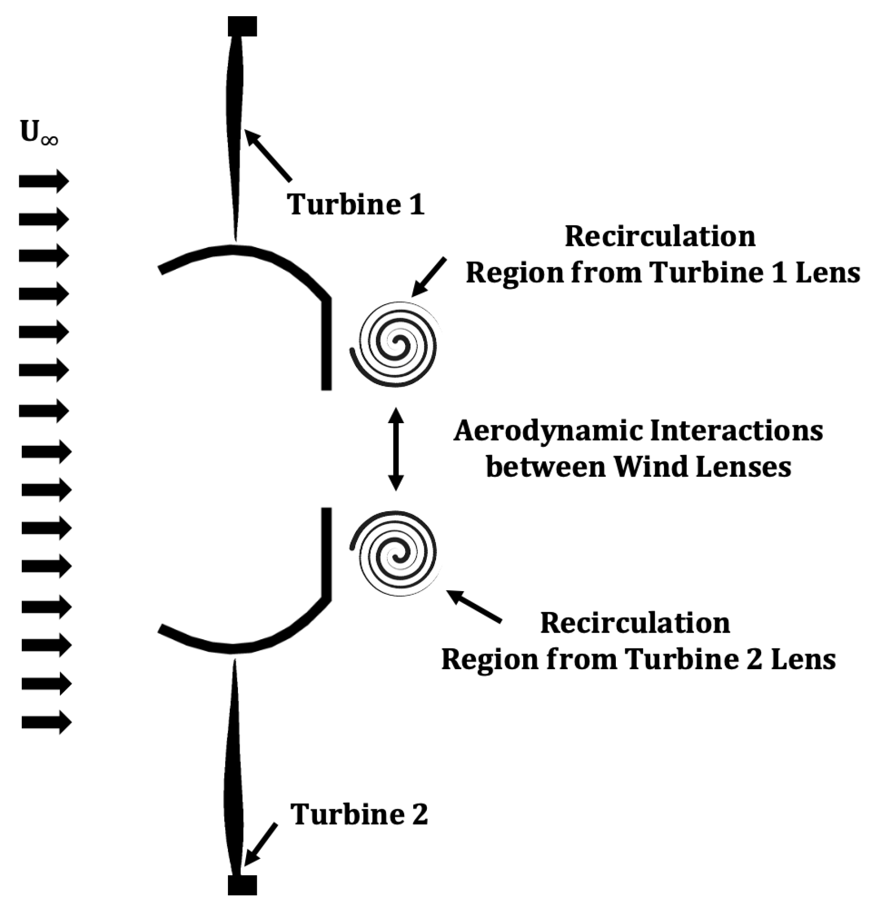
1.3. Aerodynamic Interactions between Bluff Bodies

Despite the increment in power per lensed turbine when placed in a grid of lensed turbines, the aerodynamic interactions that lead to the increment in power remain largely unexplored. However, it is hypothesized that the dynamics of the interaction largely resemble those of side-by-side bluff bodies such as circular cylinders, square cylinders, and flat plates at 90° angle of attack. Flows behind two circular cylinders of equal diameter have been investigated by various researchers over several decades [14,15,16,17,18]. One key feature is the occurrence of asymmetric wakes at critical distances of 1.5 < T/d < 2.0, where T is the transverse distance between the cylinder centers and d is the cylinder diameter [19,20]. The asymmetry is characterized by a narrow and a wider wake behind identical cylinders placed at close proximities. The narrow wake corresponds to lower base pressure, higher vortex frequency, and higher drag force, while the wide wake represents the opposite [21,22]. Similar behavior was also observed in the wake of two flat plates at 90° angle of attack [23], where significant changes in the shedding frequency was observed as a function of transverse distance. Similar to circular cylinders, increment in drag coefficient on a pair of square cylinders in a side-by-side arrangement was observed with a decrease in transverse spacing between the cylinders [24]. The pressure distributions on two cylinders with triangular cross section in a side-by-side arrangement have also been shown to experience asymmetric drag coefficients as a function of transverse distance between the cylinders [25]. Half-span models of cylinder pairs in a flow field were also shown to exhibit similar wake asymmetry characteristics with a slight suppression of vortex shedding from the cylinder surface by the trailing vortex emanating from the free end [26]. In general, it has been shown that the interference between two bluff bodies in a side-to-side arrangement is detectable when the gap width (distance between the wakes of the bluff bodies) is less than five times the diameter of the cylinder [14]. The above-mentioned studies indicate the presence of wake asymmetry and changes in wake signature when two identical bodies are placed at close proximities to each other in an uniform flow. A similar behavior is also expected for profiles of wind lenses in a lensed turbine. However, to the best of the authors’ knowledge, the extent of asymmetry and the interactions with the geometric features of the wind lenses have not been characterized.
Therefore, the objective of the current research is to quantify the aerodynamic interactions between two wind lens profiles of various geometries without the influence of turbines. The study only focuses on the lens shapes and their interactions. The influence of a spinning turbine will be explored in future work with three-dimensional particle image velocimetry (PIV).

2. Experimental Setup

2.1. Wind Tunnel

All experiments were conducted at the University of Dayton Low-Speed Wind Tunnel (UD-LSWT) in the open jet configuration. The UD-LSWT has a contraction ratio of 16:1 with 6 anti-turbulence screens. The freestream turbulence intensity is below 0.1%, measured by hotwire. The test section velocity varies from 3 m/s to 40 m/s. The open jet test section inlet measures 76.2 cm × 76.2 cm (30 in × 30 in) and opens into a pressure-sealed plenum. The effective test section length is 182 cm (72 in). The freestream velocity is measured using a Pitot tube connected to a TSI Micromanometer (Model 5825).

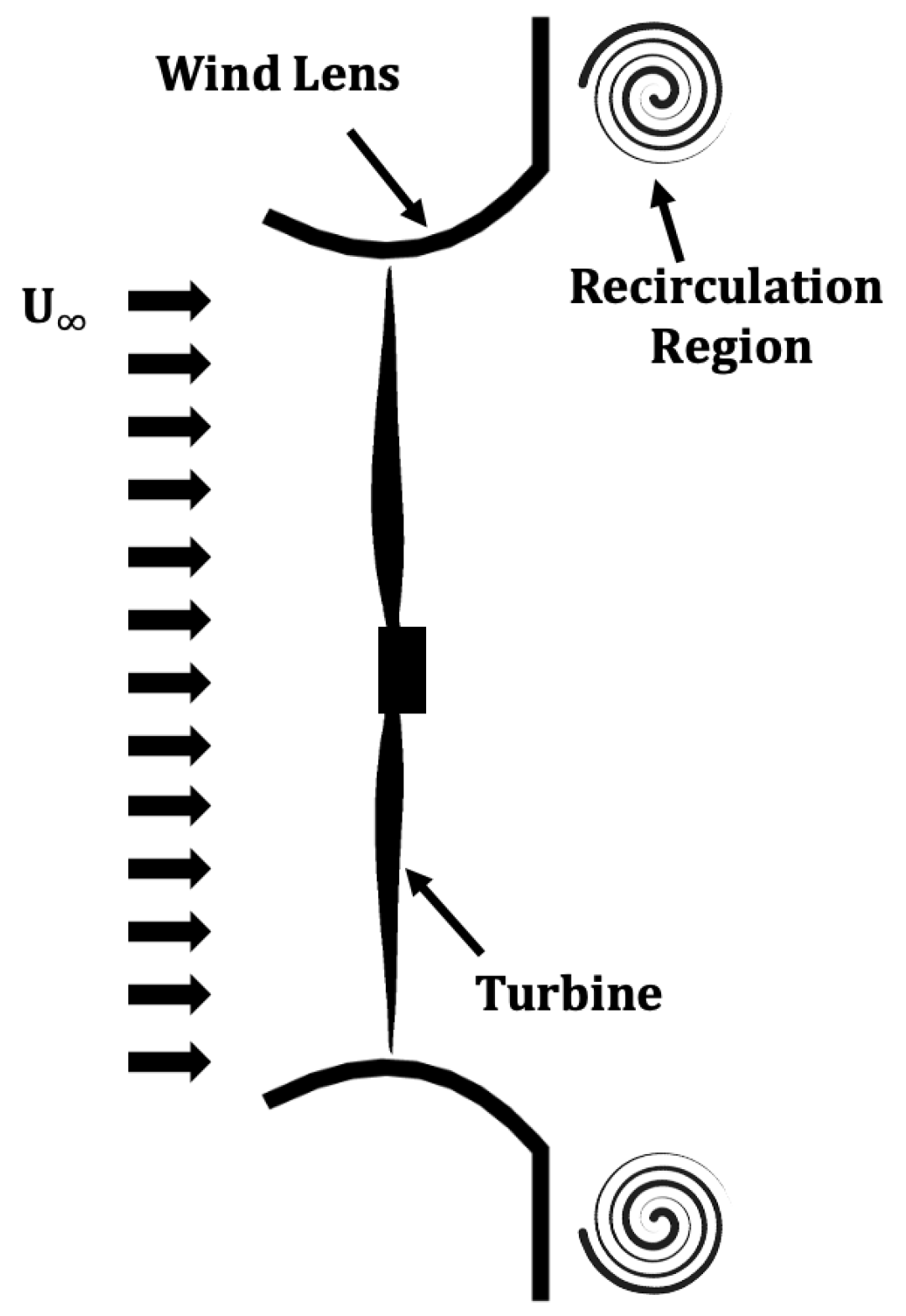
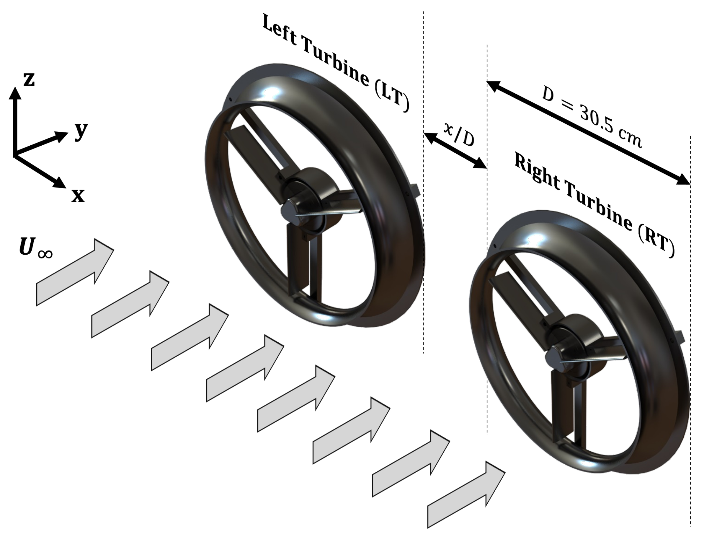
2.2. Wind Lens Models
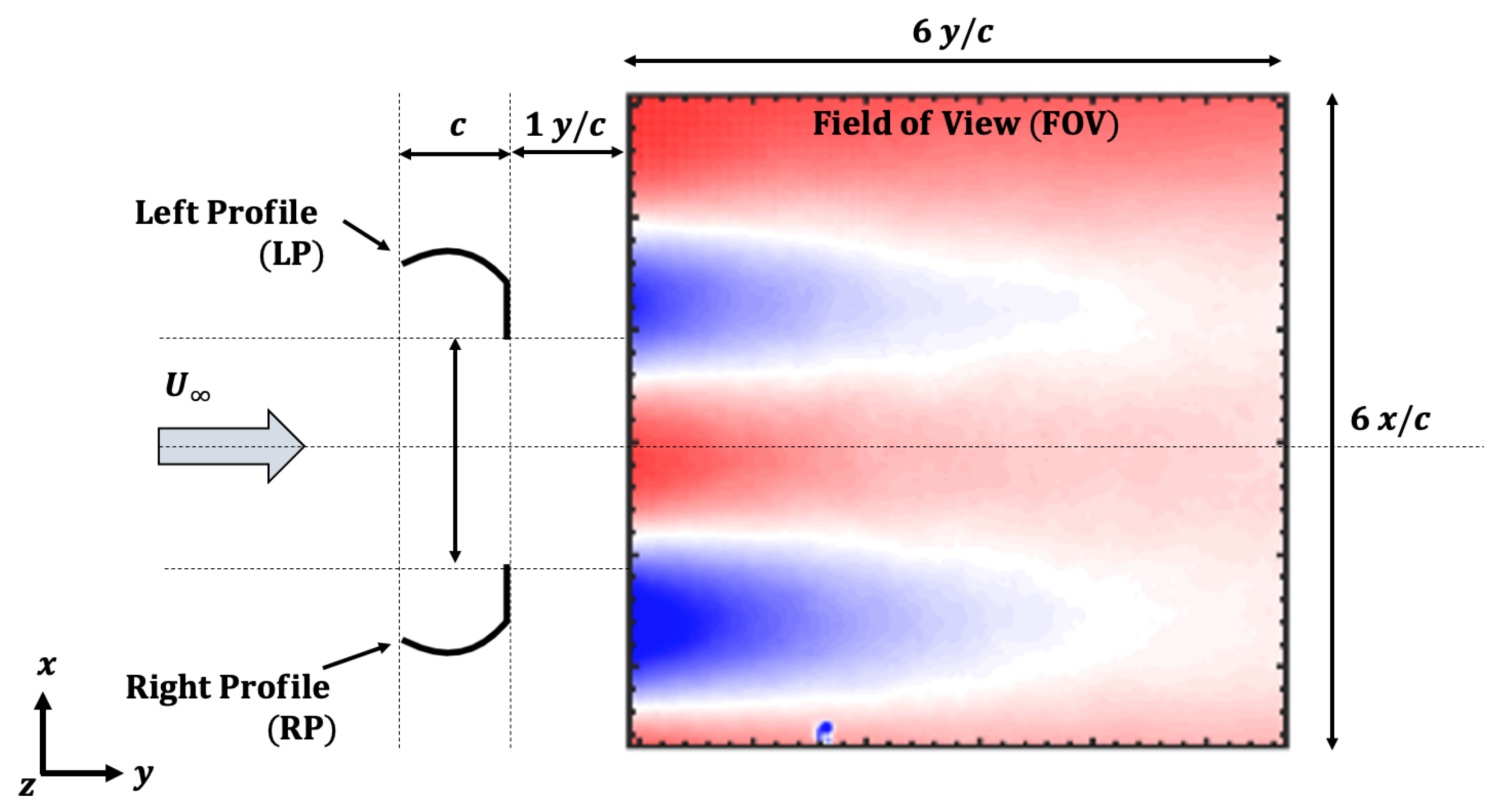
The aerodynamic interactions between wind lenses were determined by experimentally testing three lens profiles with different geometries. The specifications and the geometry of each lens profile are discussed in this section and are shown in Figure 5 and Figure 6. In Figure 5, c represents the chord length of the lens which was set to 2.54 cm (1 in), h is the height of the brim, R is the rotor radius, which was chosen to have the same value as indicated in [13] to be 15.25 cm, and R N and R D represent the inlet and exit radius of the lens, respectively.
Table 1 shows the geometrical features of all three lens profiles. A major difference in the lens geometries is the brim height, with Profile 2 having the highest value. The distance between the leading and trailing edges L T of all three lenses was 1 inch. Table 1 also shows the performance of the lens profiles reported in [7] in terms of coefficient of power ( C P ) and coefficient of drag ( C D ). Profile 2 shows the highest power coefficient and drag coefficient; however, Profile 1 produces greater C P for a given C D . These profiles were chosen for the lens–lens interactions since they will have drastic differences in their wake signature.

2.3. PIV Setup

The aerodynamic interactions between the two wind lenses were investigated through particle image velocimetry (PIV) at a freestream velocity of 10 m/s. To quantify the effects of the lens proximity without any three-dimensional effects, the turbines were not placed inside the lenses. The schematic of the PIV setup is shown in Figure 7. The field of view (FOV) was placed behind the two wind lenses to capture the wake interactions. The size of the FOV was 161.5 mm × 161.5 mm (6.36 in × 6.36 in), with a spatial resolution of 12.83 pix/mm (12,830 pix/m). The PIV experiment was conducted using a Vicount smoke seeder with glycerin oil, a 200 mJ/pulse Nd:YAG frequency doubled laser (Quantel Twins CFR 300), and an Imperx B2021 camera with 100 mm lens. The time delay between the laser pulses was set to obtain an average particle displacement of 8 to 10 pixels in the wake of the lenses and was found to be 94 microseconds (0.000094 s).
A Powell lens was used to open the laser beam into a sheet. The laser and camera were triggered simultaneously using a Quantum composer pulse generator. In each test case, 1000 image pairs were obtained. The PIV images were processed using ISSI Digital Particle Image Velocimetry (DPIV) software. Two iterations were performed in post-processing PIV images, with 64-pixel interrogation windows in the first iteration and 32-pixel interrogation windows in the second iteration with 50% overlap. The uncertainty in the velocity measurements obtained from image capturing and processing through DPIV was determined using the process outlined by Lazar et al. [27,28]. Using this process and the parameters used in the PIV setup, the overall mean uncertainty was determined to be ±0.2 m/s.

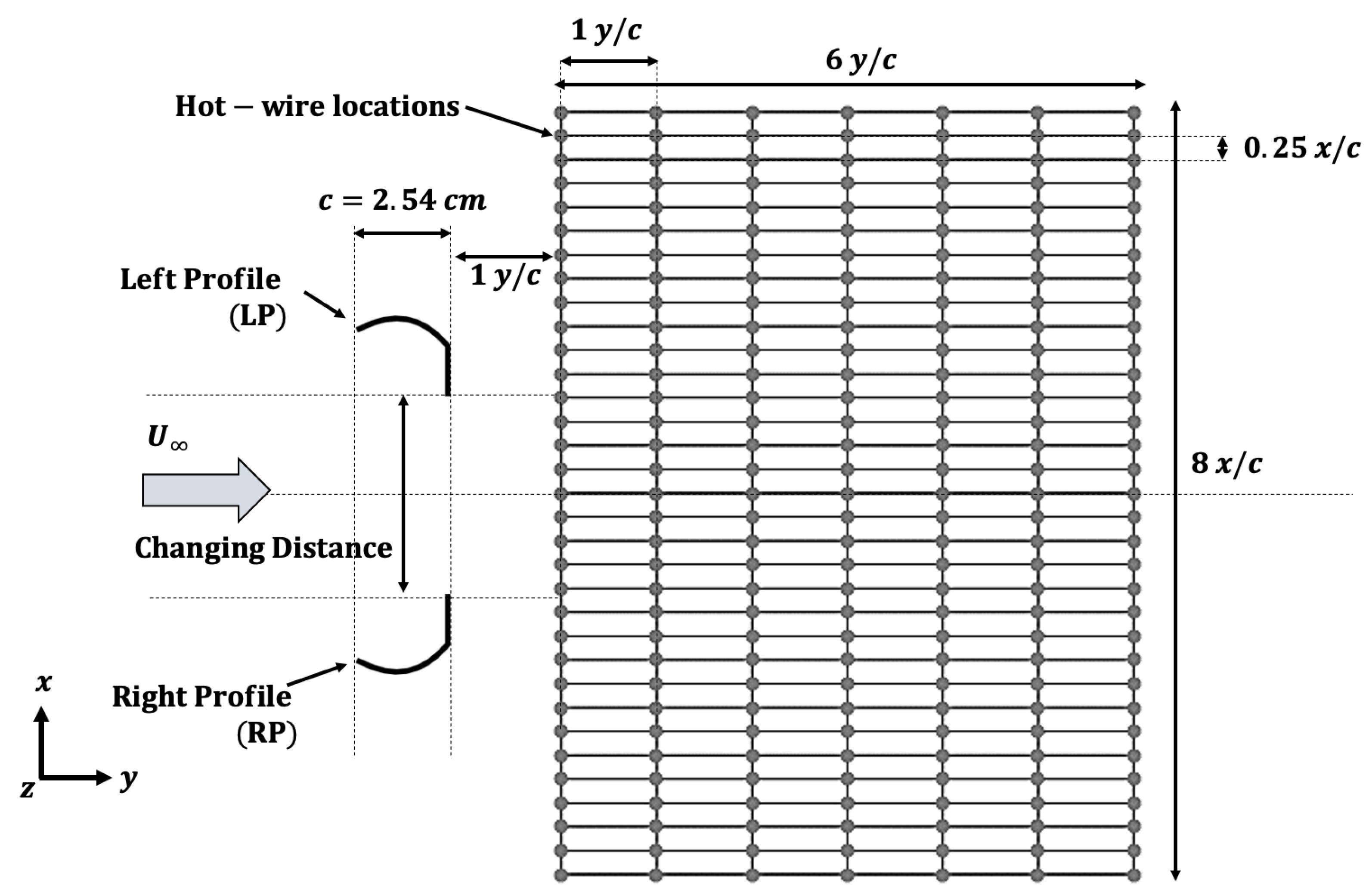
2.4. Hotwire Anemometry Testing

The hotwire experiments were performed using a Dantec hotwire probe (type 55), with an overheat ratio of 0.45 for a wire temperature no greater than 300 °C. The hotwire was placed at various downstream locations from the lens models (1–6 y/c) and traversed laterally at 0.25 x/c increments to collect data of the flow field downstream of the models, as shown in Figure 8. The traverse used was a UniSlide motor-driven assembly (model MA40), powered by a Velmex VXM-1 Stepper Motor. Data were collected using the MATLAB Data Acquisition Toolbox (DAQ).

3. Results

3.1. PIV Results

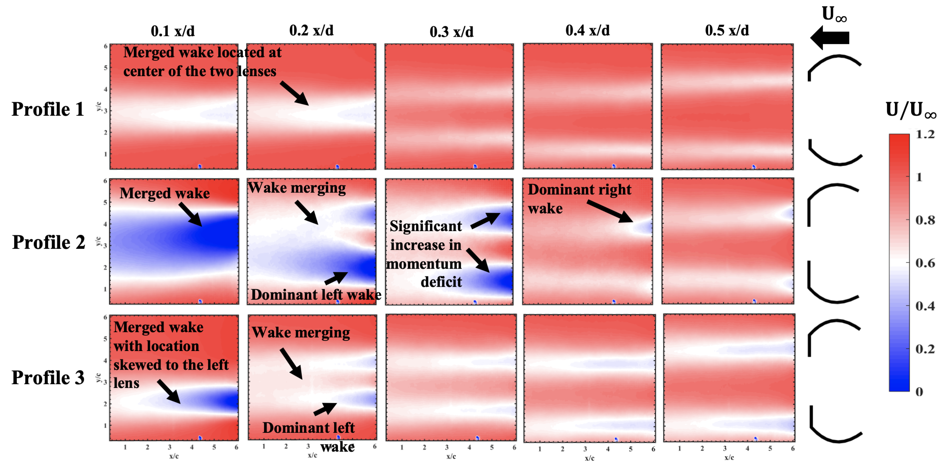
3.1.1. U Velocity Results

The results from PIV are shown in this section for the three lens profiles tested. The mean velocity contours shown in Figure 9 illustrate the mean interaction between the wake of the two identical lens profiles at different x / D spacings. At a x / D of 0.1, Profile 2 has a larger velocity deficit when compared to both profiles 1 and 3. This trend is continued in all the other x / D cases. However, several distinctions in the wake behavior can be elucidated from Figure 9. All lens profiles start with two distinct and independent wakes at 0.5 x / D . The momentum deficit magnitude is directly related to the drag coefficient of each individual lenses. At 0.4 x / D , slight changes in the momentum deficit can be observed for profiles 2 and 3 with the right (with respect to the freestream) lens showing a slightly higher momentum deficit than the left lens. Reducing the spacing even further to 0.3 x / D , there is a drastic change in the magnitude of momentum deficit for Profile 2 by almost 20%, while the magnitude of momentum deficit for profiles 1 and 3 remains the same. Strong deviations can be seen between the lens profiles at 0.2 x / D spacing. At this spacing, Profile 1 exhibits only one wake, indicating that the once-independent wakes have merged into each other. The location of the “merged” wake seems to be at the center of two lens profile locations. The wakes of Profile 2 and Profile 3 do not seem to be merged at 0.2 x / D , but the wakes from Profile 2 seem to partially merge with each other. Distinct wakes emanate from each lens independently, but within 0.3 x / D , the two wakes merge into one. At 0.1 x / D , all lens profiles exhibit only one wake, indicating that the wakes are merged.
However, the location of the merged wake with respect to the lenses are different. The merged wake location in profiles 1 and 2 seems to occur in the centerline of the FOV where the two lenses meet. However, Profile 3 shows a highly skewed wake location where the merged wake is seen behind the left (with respect to the freestream) lens profile. There is almost no indication of the presence of the right lens in the Profile 3 case at 0.1 x / D . As seen in Figure 3, the highest increment in C p is around x / D of 0.1, below which the increment in C p decreases. Therefore, a strong correlation can be made between the C p increment observed at x / D of 0.1 and the mean aerodynamic interaction of the wake.

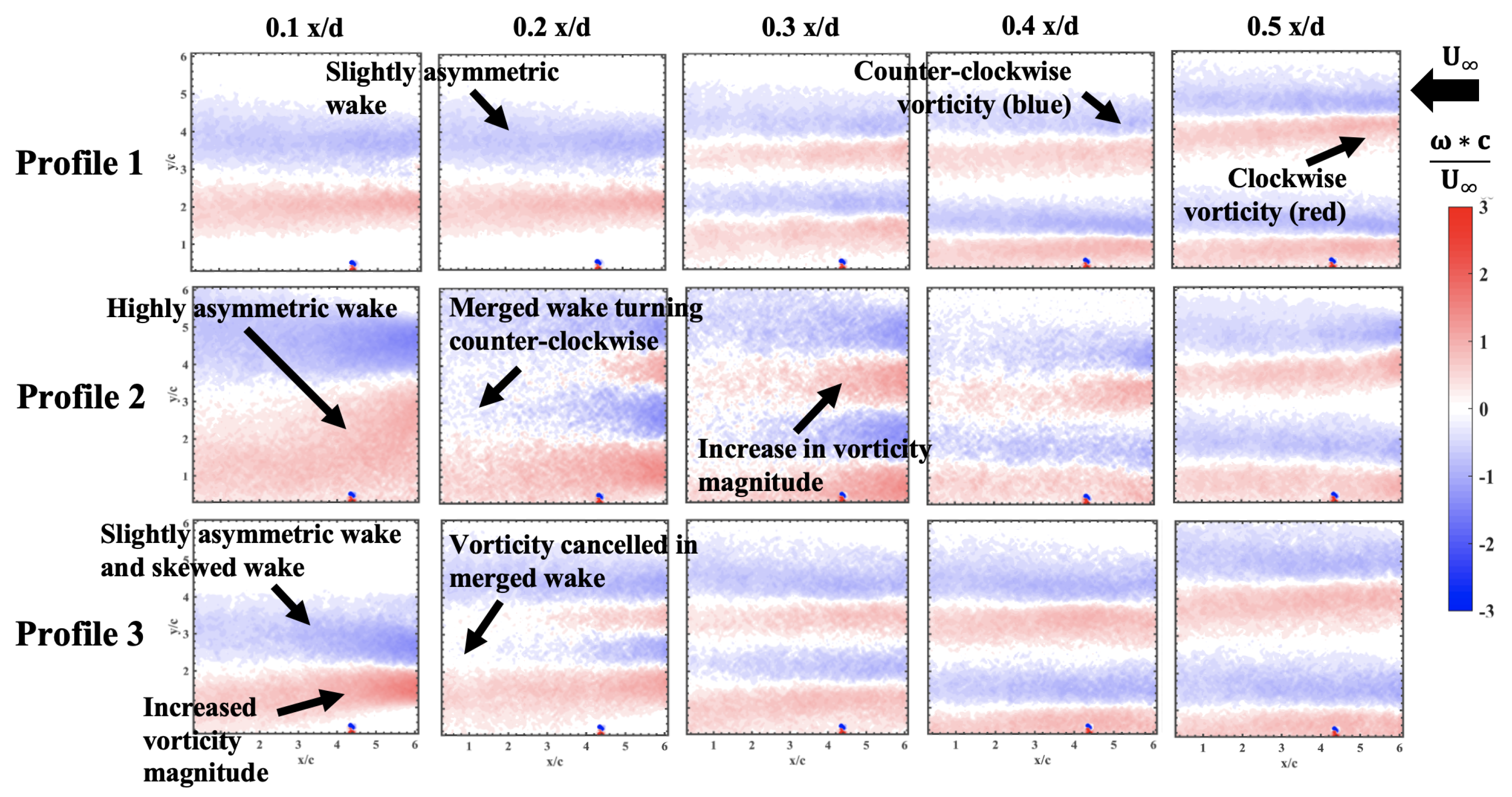
3.1.2. Mean Vorticity Results

The mean vorticity contours shown in Figure 10 follow similar trends to those of the U-velocity contours. The two bands of alternate vorticities can be seen behind each lens for all three lens profiles. The red vorticity region indicates clockwise rotation, and the blue vorticity region indicates counterclockwise rotation. At 0.5 x / D , the wakes of the Profile 1 lens pairs seem farther apart than Profile 2 and Profile 3 lens pairs. This could be because Profile 1 has a lower drag coefficient, as indicated in Table 1 and thus has a smaller momentum deficit and a thinner wake when compared to the other two lens profiles. No tangible differences can be seen in the vorticity magnitude for the two lens pairs in all three lens profile cases. Even though one of the wakes seems to dominate in the U velocity contours, the vorticity magnitude remains almost equal for all three lens pairs. However, a significant jump in vorticity magnitude can be seen for Profile 2 at 0.3 x / D which also corresponds to a significant increase in momentum deficit, seen in Figure 9. The merging of the wakes can be seen for all three lens profiles at 0.2 x / D . The merged wake has a counterclockwise rotation (blue) for Profile 2, which could be due to the fact that the upper surface vorticity (blue) of the left lens has a slightly stronger magnitude than the lower surface vorticity (red) of the right lens such that the resultant wake has a net counterclockwise rotation after merging. In the case of Profile 3, these two vorticity bands from the lens pairs cancel each other, resulting in an almost irrotational flow. This could be one of the reasons why the merged wake ends up skewed to the left lens instead of occurring at the center of the two lenses.
The symmetry of the wake can also be visualized in Figure 10, in all lens profile cases at higher x / D spacings. All three lens profiles seem to exhibit a symmetric wake profile at 0.5 x / D and maintain symmetry until merging at 0.2 x / D . After merging, the wake profiles tend to be slightly asymmetric in the case of profiles 1 and 3, whereas high asymmetry can be seen in the case of Profile 2. The vorticity contours clearly show that the dynamics of wake merging are strongly dependent on lens geometry and offer insight into the skewness and asymmetry of the wake after merging.

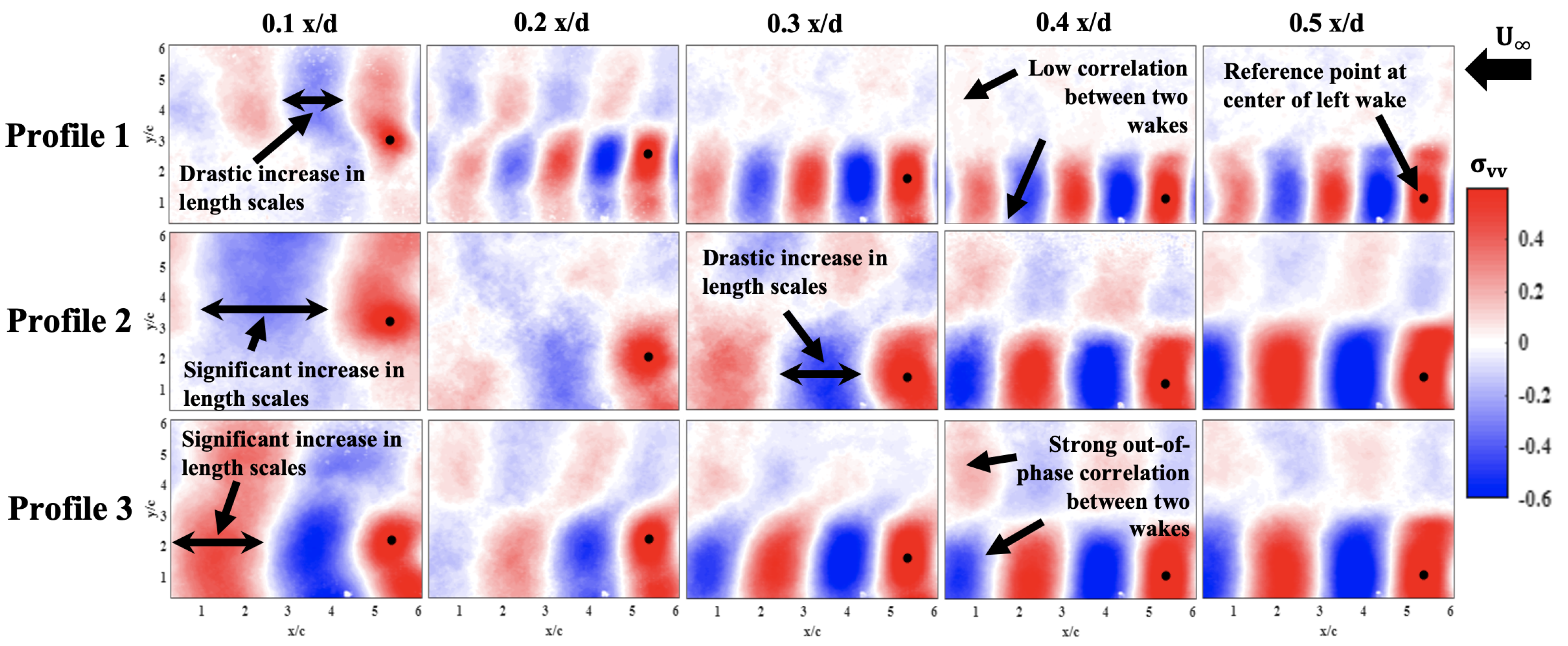
3.1.3. Two-Point Correlations

It is well known that the vortex shedding frequency and turbulent length scales contribute to turbulent-induced pressure fluctuations, sound generation, and structural vibrations [29]. The lens proximity effects in the wake and its influence on the vortex shedding frequency and the corresponding length scales can be determined by performing two-point correlation of fluctuating velocities in the wake. Bendat and Piersol [30] defined the two-point correlation as
ρ u i u j = [ u i ( X 1 , t ) u j ( X 2 , t + τ ) ] u i ( X 1 ) 2 ¯ u j ( X 2 ) 2 ¯
where X 1 and X 2 are two spatial locations in the PIV field of view, τ is the time delay (which is chosen to be zero for the results shown below), and u’ represents the fluctuating velocities in i and j directions. The two-point correlations for the V velocity component are shown in Figure 11 for all three lens profiles at different x / D spacings. The reference point X 1 was chosen to be at the center of the wake of the left (with respect to the freestream) lens. The alternate band of correlations can be seen for all cases in Figure 11, which illustrates the presence of coherent structures that are shed from the lenses and their corresponding length scales. At 0.5 x / D , it can be seen that Profile 1 exhibits a lower length scale and higher frequency coherent structures when compared to profiles 2 and 3.
While reasonable out-of-phase correlations persist between wakes of the left and the right lenses for profiles 2 and 3, the correlations between the left and right wakes are less pronounced in the case of Profile 1. As the distance between the lenses are decreased at 0.3 x / D , Profile 2 exhibits a drastic increase in the length scales which has a strong influence in the mean velocity and vorticity magnitude, as seen in Figure 9 and Figure 10, respectively. No such changes are seen for profiles 1 and 3 at 0.3 x / D . At 0.2 x / D , all lens profiles exhibit a loss in the strength of the correlations when compared to higher x / D cases. This could be due to the wakes merging into each other. Apart from changes in correlation magnitude, Profile 1 exhibits a decrease in length scales as 0.2 x / D , when compared to 0.3 x / D . No such changes in the length scales are seen in profiles 2 and 3 at 0.2 x / D . However, the merged wakes on all three lens profiles for 0.1 x / D show a drastic increase in the length scales, with Profile 2 exhibiting a significant increase. The two-point correlations show that the merged wake of Profile 1 is slightly skewed to the right lens instead of the left, as seen in Profile 3. These correlations provide strong evidence to fundamental changes in the wake signature as profile geometry and proximity changes. Based on these observations, significant conclusions can be drawn not only about the downstream properties in the area of interest between the lens profiles, but also, perhaps most importantly, the increment in power identified by Novotny and Gunasekaran [13] and as indicated in Figure 4.

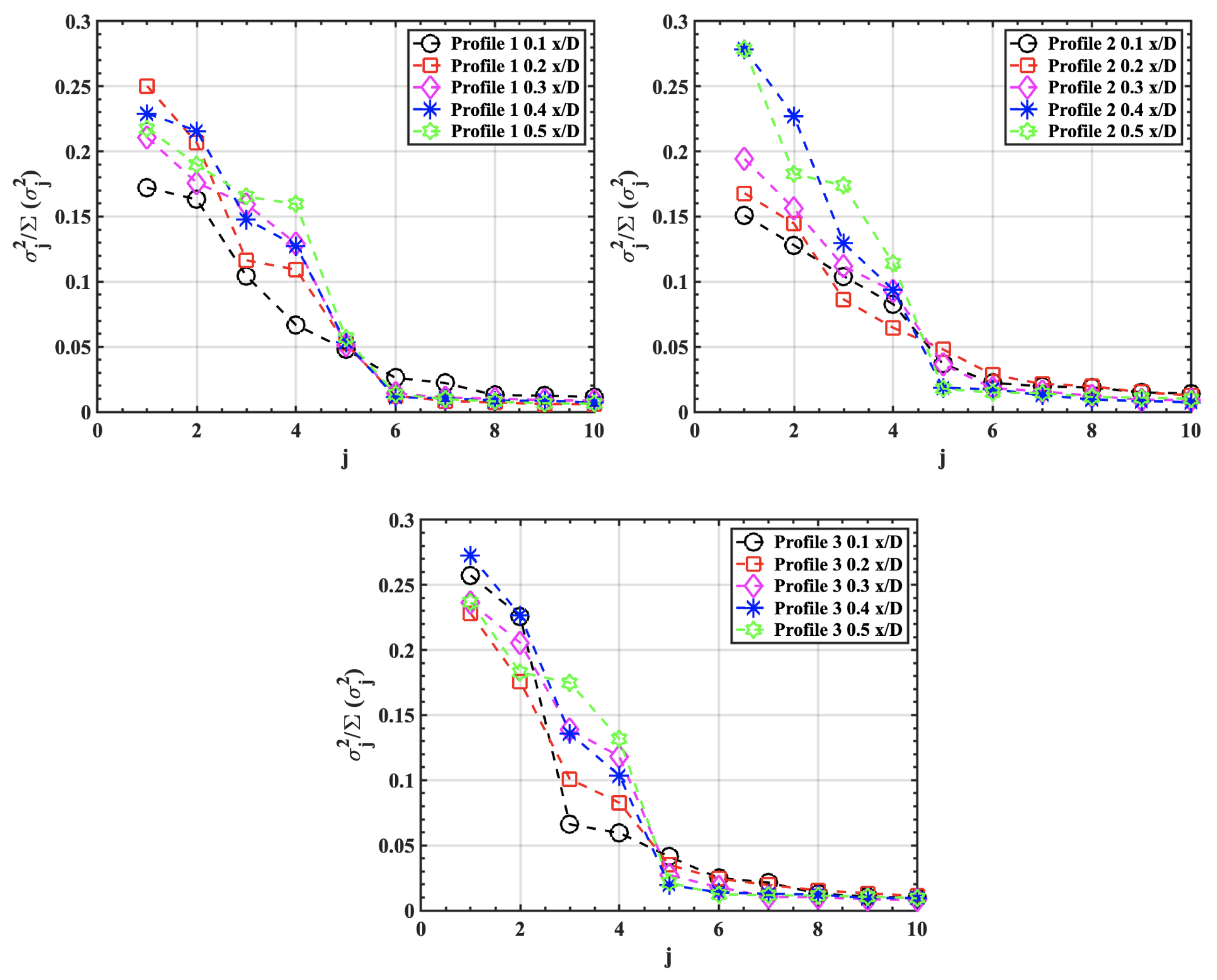
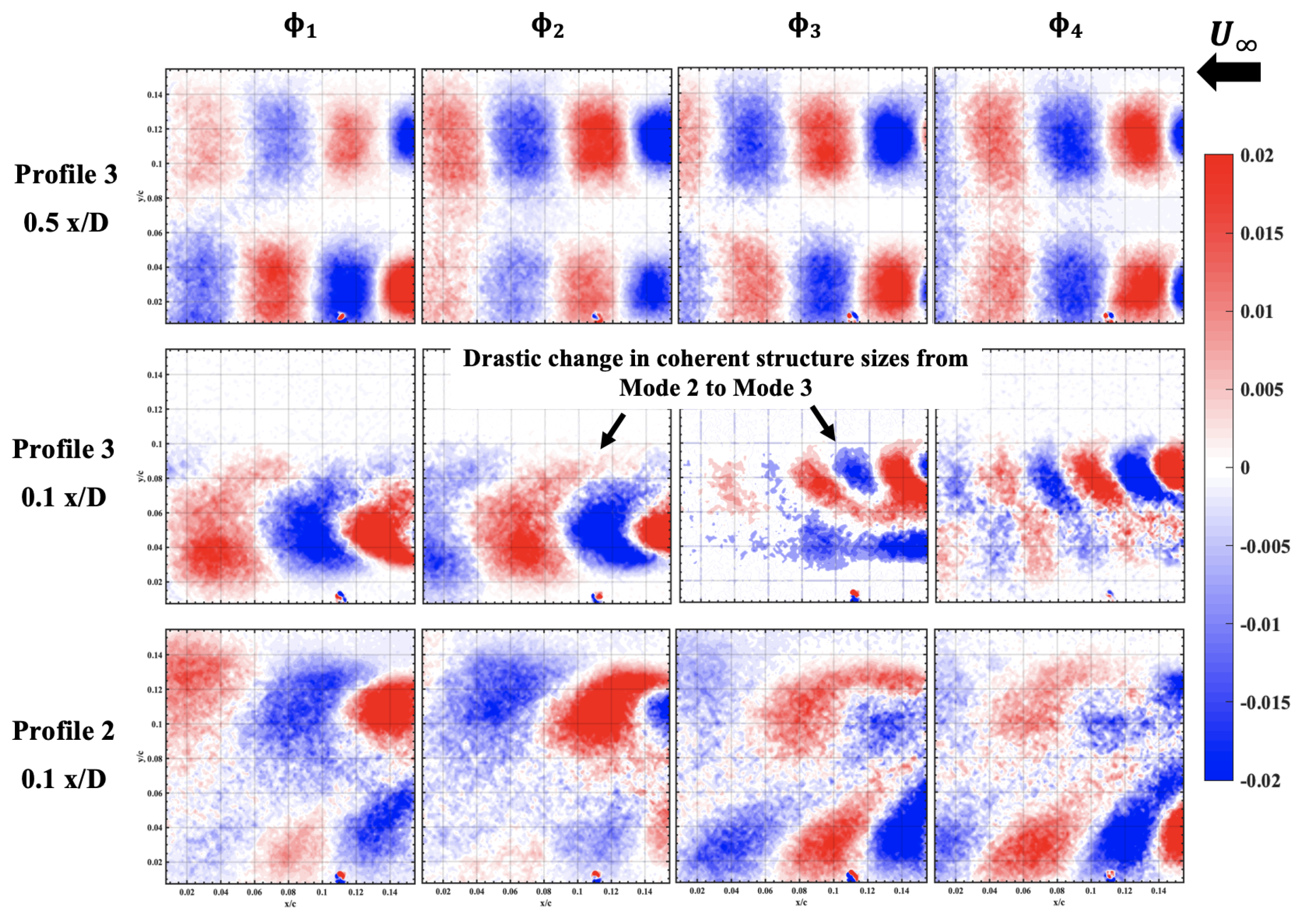
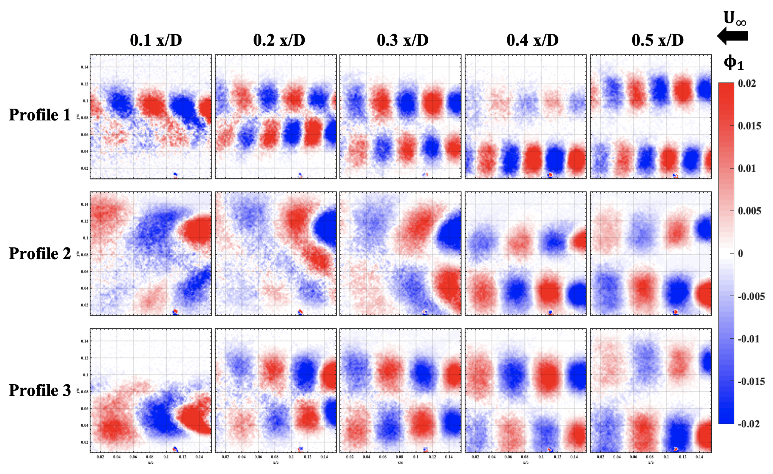
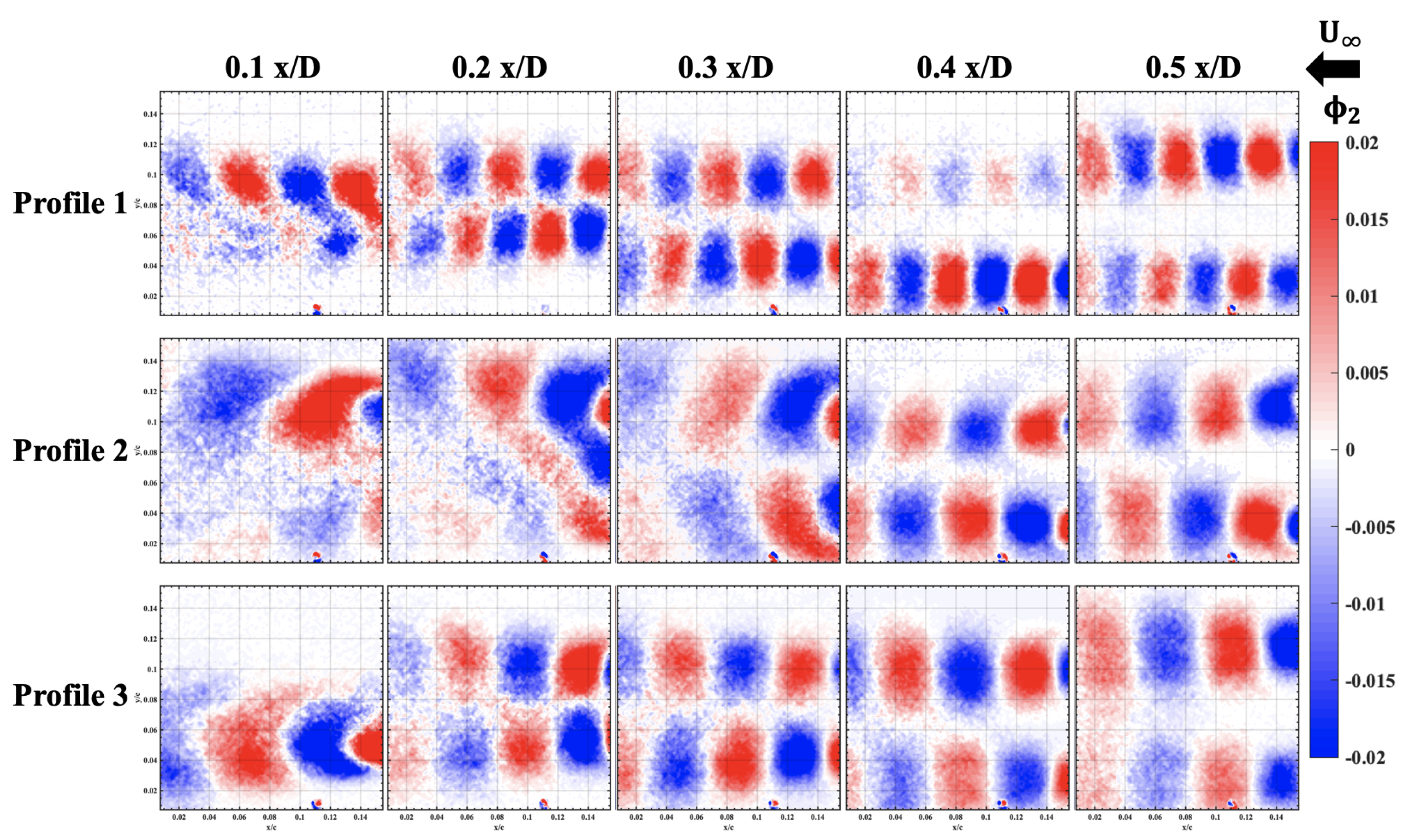
3.1.4. Modal Analysis

While the two-point correlations show the presence of coherent structures, the results shown in Figure 11 depend on the selection of reference points with respect to which the correlations are performed. Selection of a different reference point in the wake will yield different results. As such, proper orthogonal decomposition (POD) was conducted on the wake vorticity to truly reveal the presence of the dominant modes in the wake of the lens pairs at different x / D spacings. The POD, also known as principal component analysis (PCA) or the Karhunen–Loéve (KL) expansion, is a singular value decomposition (SVD)-based technique often used to generate a low-rank, orthogonal basis that optimally represents a set of data. To generate a complete set of POD modes, the fluctuating vorticity data from PIV were compiled and represented as matrix X where the columns represent snapshots in time. The size of the X matrix is m×n. In the present case, the m = 14,161, which represents the reshaped field of view data in each time step into a single column, and n = 1000, which represents the number of images taken. The SVD was then used to factorize the matrix X into three matrices, as shown in Equation (2).
X = U Σ V
where U C ( m x n ) , V C ( n x n ) and Σ R ( m x n ) , and the asterisk denotes the conjugate transpose. The Σ matrix consists of only diagonal elements that represent the singular values of X represented by σ . The U and V matrices consist of the eigenvectors of the covariance matrices X X and X X , respectively. As a result, the SVD allows the decomposition of X into
χ k = j = 1 n σ j u k j ϕ j
assuming that m > n . Hence, Equation (3) shows that the SVD returns a complete orthonormal set of basis functions for the vorticity matrix X. The elements of this basis are the vectors ϕ j and are referred to as the POD modes [31]. The relative importance of the jth POD mode ϕ j is determined by the relative energy E j of that mode, defined as [31].
E j = σ j 2 i = 1 n σ i 2
where the total energy is normalized such that j = 1 n E j = 1 . The relative energy obtained from Equation (4) using the singular values of the mean subtracted vorticity matrix for all three lens profile cases at different x / D spacing is shown in Figure 12. It can be seen that modes 1 to 6 are shown to be the most dominant in terms of relative energy. The relative energy plateaus to near-zero value at modes greater than 6, except for the lower x / D case. For Profile 1, as the spacings between the lens pairs are reduced, the relative energy of the dominant POD modes also reduces. However, this reduction in the relative energy at lower POD modes is compensated by the increase in relative energy at higher POD modes, as seen clearly in the 0.1 x / D case. Similar trends in the relative energies can be observed in the Profile 2 lens as well. With decrease in x / D spacing between the lenses, the relative energy in the lower POD modes decreases. The relative energy variation of the POD modes in the Profile 3 case shows similar behavior as compared to profiles 1 and 2, except at modes 1 and 2. The strength of the POD modes decreases with decrement in lens spacing until the 0.2 x / D case. At 0.1 x / D , the strength of the POD modes 1 and 2 is comparable to 0.4 x / D and shows drastic decrease at mode 3. The higher relative energy in mode 1 and 2 is possibly due to a comparatively large-scale vortex shedding in the Profile 3 wake at 0.1 x / D spacing, as shown in Figure 9 and Figure 10, respectively. However, the relative energy in Mode 3 in 0.1 x / D spacing drastically decreases when compared to the relative energies in mode 1 and 2, following similar behavior as seen in the 0.1 x / D cases of profiles 1 and 2.
The trends seen in relative energies shown in Figure 12 are better visualized using the POD contours. Figure 13 shows the first four dominant modes for Profile 3 at 0.5 x / D and 0.1 x / D and for Profile 2 at 0.1 x / D . The POD mode contours are similar to the two-point correlation contours, where alternating red and blue bands are seen which represent the alternate shedding of coherent structures in the wake of the lens pairs. Gradual decrease in the relative energy for Profile 3 at 0.5 x / D , seen in Figure 12, can be correlated with similar coherent structure sizes seen in the first four modes shown in Figure 13. At 0.1 x / D , however, there is a drastic change in the size of the coherent structures from mode 2 to mode 3 that corresponds to a sharp decrease in the relative energy seen for this case in Figure 12. The first four POD modes for Profile 2 case at 0.1 x / D did not result in drastic change in coherent structures, hence a gradual decline in the relative energy is seen in Figure 12. Profile 1 also shows similar behavior to that of Profile 2.
The first two POD modes for the three lens profiles at different x / D spacings are shown in Figure 14 and Figure 15, respectively. Figure 14 shows the first mode, the mode with the highest relative energy. Drastic increase in the size of the coherent structures can be seen in the POD mode 1 contours with decrease in lens spacing. The increase in the coherent structure sizes is responsible for the comparable decrease in the relative energy seen in Figure 12 at 0.1 x / D lens spacing.
The POD mode 2 contours for all three lens profile cases are shown in Figure 15. The mode 2 contours are extremely similar to the trends seen in mode 1 contours, except that they exhibit a lower relative energy, as seen in Figure 12. The modal analysis clearly shows that the wake signature changes drastically as the spacing between the lens pair changes. At close proximities around 0.1 x / D , the relative energy of the dominant modes decreases and the overall energy is distributed over higher number of modes, whereas higher x / D spacing only requires six modes for capturing 99% of the overall energy in the flowfield.

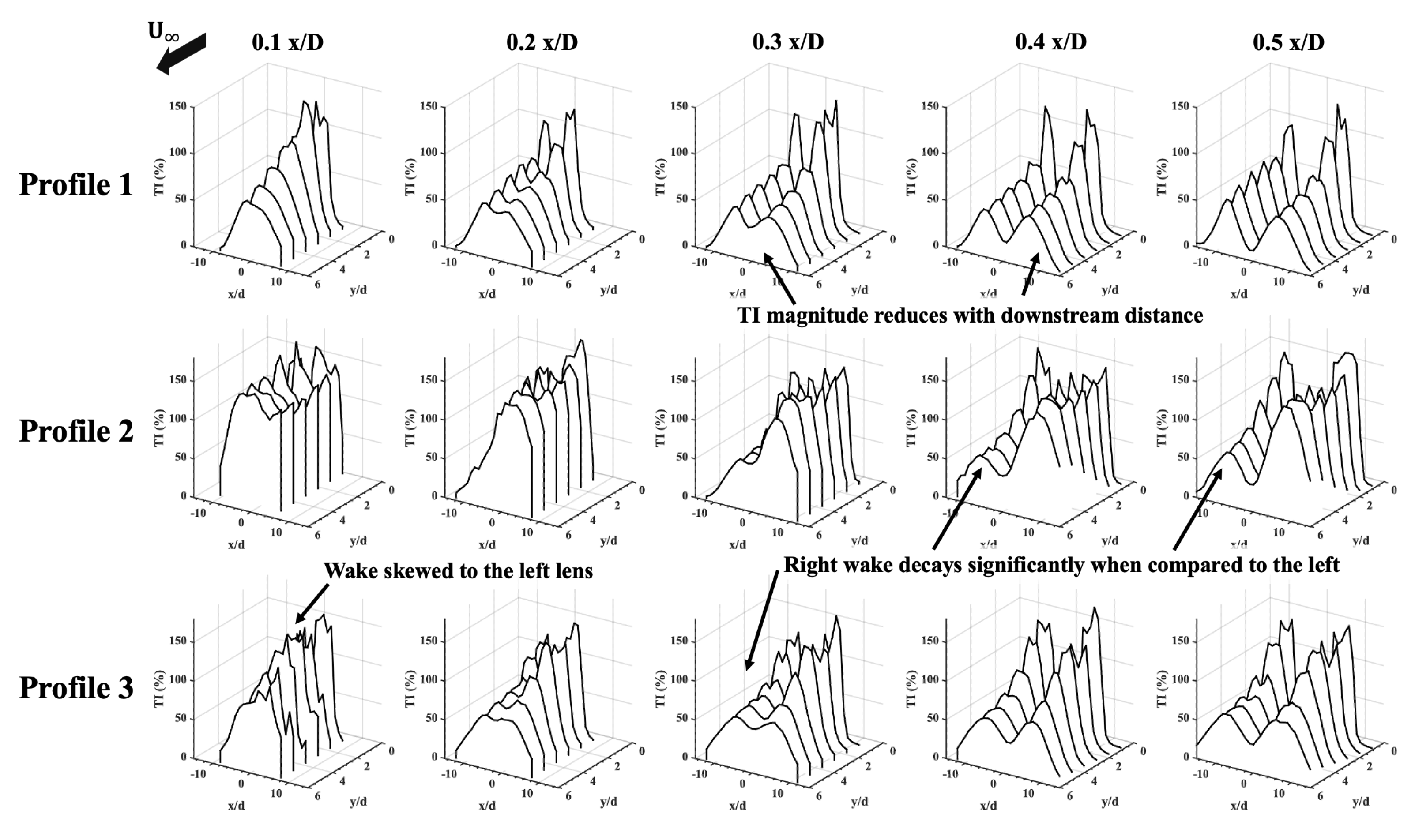
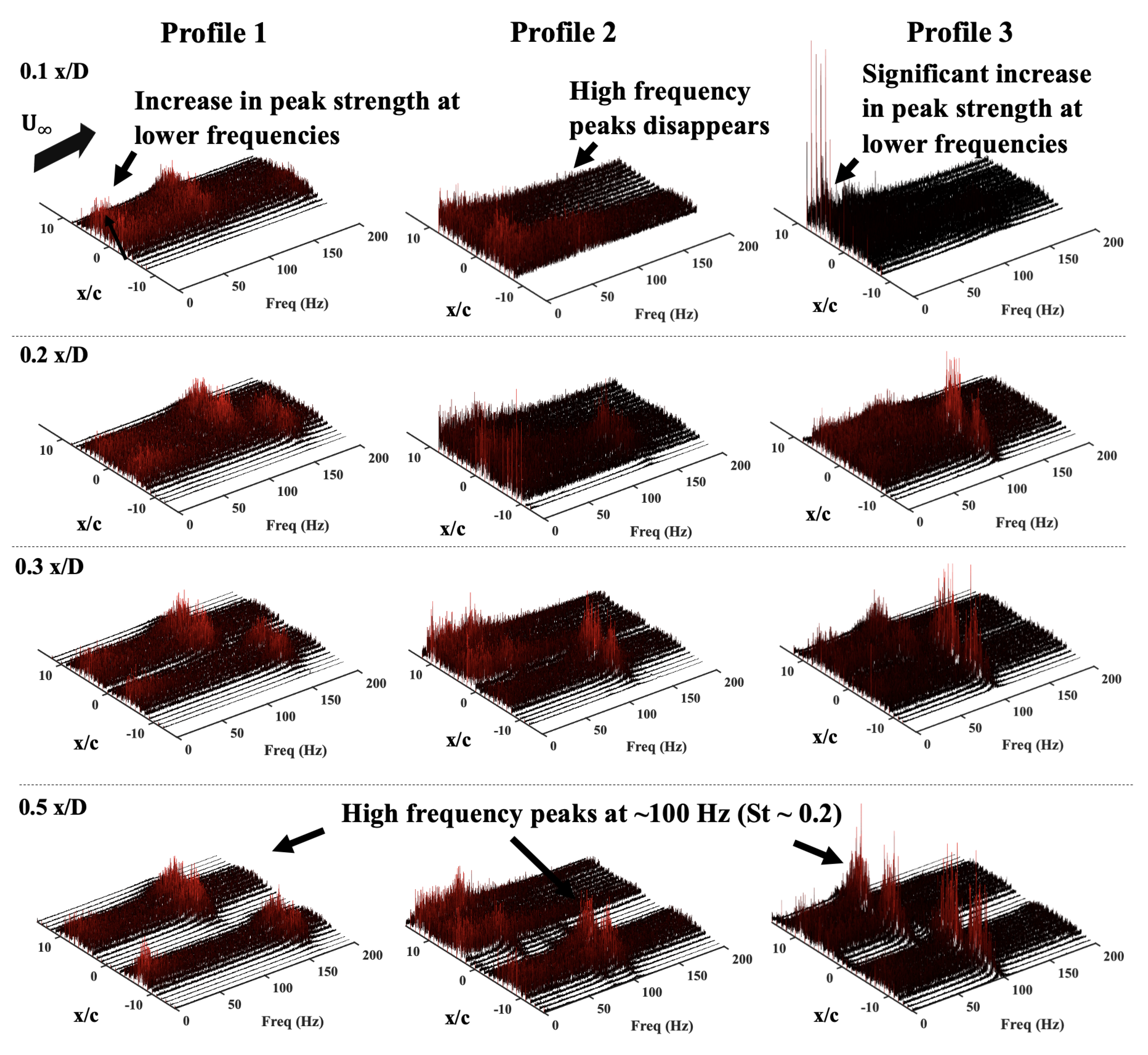
3.2. Hotwire Anemometry Results

The temporally resolved hot-wire data were used to determine the turbulence intensity and the spectral content of the wake through fast Fourier transform. The turbulence intensity is calculated by Equation (5).
TI ( % ) = u 2 ¯ U 100
where u is the fluctuating velocity in the wake. The TI calculated at each grid location shown in Figure 8 is plotted as a function of x/c and y/c in Figure 16. The bimodal nature of the TI profiles at higher x / D distances clearly shows the presence of two independent wake signatures. A higher TI magnitude is seen directly behind the lenses and gradually decreases with increase in downstream distance. While the decrement in TI in the wakes of the Profile 1 and Profile 3 lens pairs show similar decay, the wakes of Profile 2 lenses show widely different behavior, where the right wake decays significantly when compared to the left wake, even at a greater lens spacing. This could be due to the higher wake width created by the Profile 2 lens, as seen in the PIV results. The decay of TI in the right lens when compared to the left becomes highly evident in Profile 3 at 0.3 x / D , indicating the merging of the wake at a downstream distance rather than directly behind the lenses. The Profile 1 case at 0.3 x / D , however, shows two stratified wake signatures without any indication of merging. At 0.2 x / D , the wakes of all lens profiles are merged, and it is at this stage where the skewness of the wake can be seen. Significant skewness in Profile 2 and Profile 3 cases can be observed at 0.2 x / D lens spacing, where the wake is skewed to the left lens. Partial skewness towards the left lens can also be observed for the Profile 1 case as well. At 0.1 x / D , the bimodal nature of the TI profile disappears as the wakes merge into one wake with a high TI magnitude. However, the TI decay rate of the merged wake is significantly lower when compared to the independent wakes of the lenses at 0.5 x / D . The skewness in the wake could be the indicator of why two wind lens turbines placed at close proximities show slightly different performance in power output. Figure 16, along with the PIV results, provides insight into the reasons why there exists a disparity in the power output between the lens pairs.
While the wake skewness could explain why one lens turbine outperforms the other, it does not explain the significant increase in the overall net power output seen in the wind lens pairs. The spectral content of the wake is investigated to determine a plausible cause for the net increment in power output. Fast Fourier transform (FFT) was performed on the velocity signals obtained from hot-wire measurements at each grid point location shown in Figure 8. The spectral content in the wake at 3 y/c downstream distance is shown in Figure 17 at various x / D cases tested. At 0.5 x / D lens spacing, all lens profile cases show a distinct wake signature for the lens pairs. The frequency spectrum at the wake of the lenses is scattered with oscillations in frequencies when compared to the freestream. The peak frequencies in all the independent wakes of each lens pairs are around 100 Hz, which corresponds to a Strouhal number of 0.2, depending on the chord of the lens. It is well known that the Strouhal number of 0.2 is the most common shedding frequency experienced in most bluff bodies. Even at a lens spacing of 0.5 x / D and 0.3 x / D , the dominant wake frequency of the left wake is lower than that of the right lens, indicating that even though the wakes may seem independent, the effect of the neighboring wake is felt in its counterpart long before the wakes are merged. At 0.2 x / D , significant changes to the frequency spectrum can be seen. The peak frequency strength around 100 Hz seems to diminish, with Profile 2 showing no peaks at 100 Hz. The strengths of the lower frequencies, however, seem to increase when compared to the higher x / D cases. At 0.1 x / D , the peak frequencies around 100 Hz completely vanish for all the lens profile cases and the prominent frequencies shift to the lower end of the spectrum. This phenomenon seems to coincide with the two-point correlation results seen in Figure 11 and in the modal analysis. At 0.5 x / D , the shorter-length scales correspond to higher frequencies, and at 0.1 x / D , the large-length scales correspond to lower frequencies.
This reduction in peak frequency phenomenon explains clearly why the performance of the turbines are enhanced at close proximities. Due to the larger shedding frequency at larger spacings between the lenses, the “resting” time of the vortex behind the lenses are shorter. As the lenses are brought closer to each other, the merging of the wake disrupts the high frequency of vortex shedding and lowers the shedding rate to lower frequencies such that the resting time of the vortex behind the lens is comparatively longer. A longer resting time of the vortex behind the lens corresponds to a more consistent lower pressure that draws air at a higher velocity at a steady rate compared to high vortex shedding frequency at larger separation distances.

4. Conclusions

Experimental investigations of lensed turbines in a side-by-side arrangement showed that the performance can be improved through strategic placement of the lenses with respect to each other. Prior work revealed the optimal spacing of the lensed turbines in a side-by-side arrangement to be 0.1 x / D . The fundamental flow physics responsible for the increased net power output from a pair of lens turbines placed at close proximity was quantified through PIV and hotwire investigations. As the two lenses are brought in close proximities to each other, the following happens:
  • The two wakes sense the presence of each other such that the peak shedding frequency for one of the wakes is lowered when compared to the other. This causes changes in the mean flow parameters such as the mean velocity and vorticity. The relative energy in the POD modes starts to decrease.
  • Reducing the spacing between the lenses further results in the onset of wake merging that causes significant changes in the vortex shedding frequency, and the size of the coherent structures in the wake starts to increase. This results in that wake having a higher momentum deficit and a higher turbulence intensity.
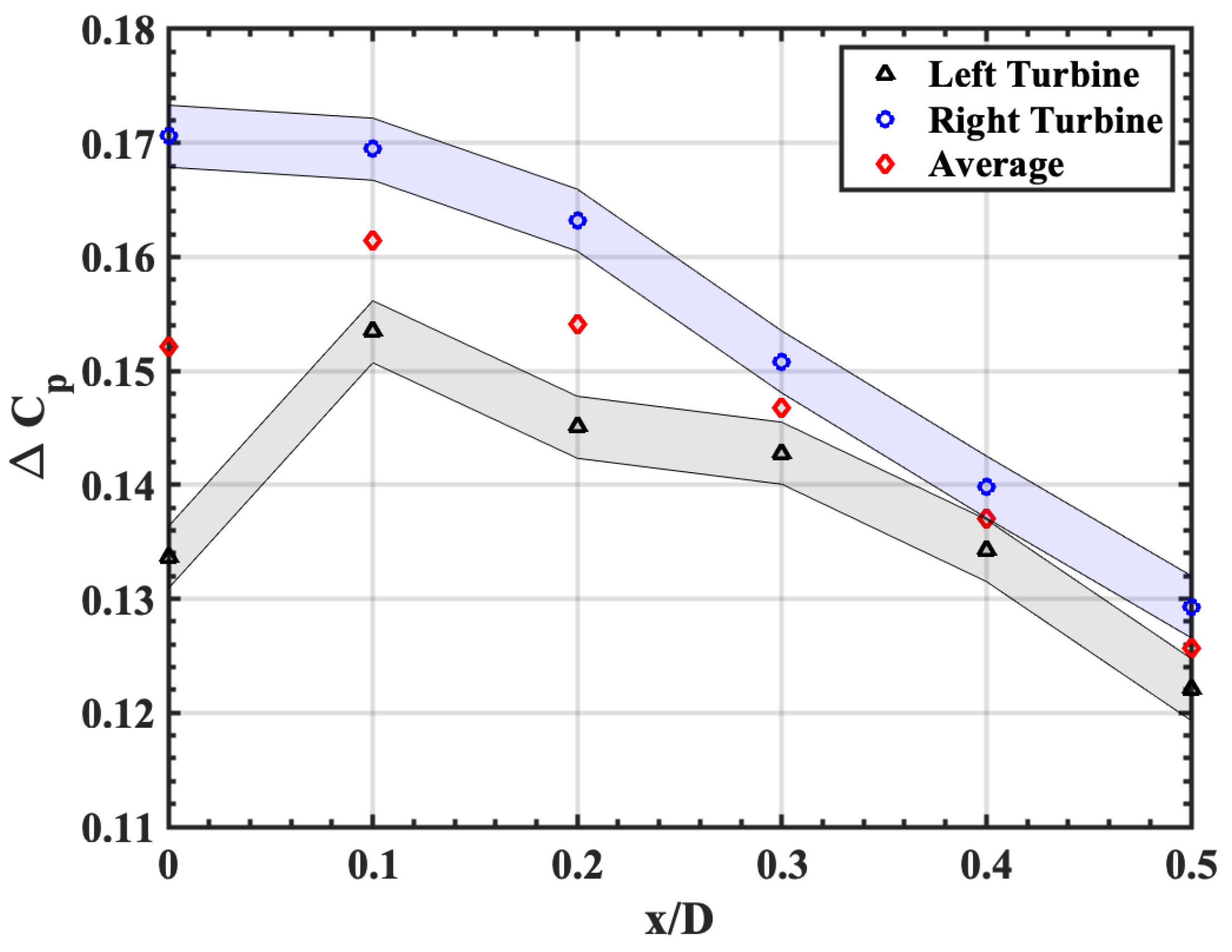
  • The choice of the direction of the skewness in the wake is hypothesized to be due to the extent of cancellation on the inboard vorticity magnitude from the two wakes. If the vorticity is perfectly canceled between the wakes, little to no wake skewness is observed. The direction of skewness of the merged wake causes one of the turbines in the lens turbine pair to outperform the other, as seen in the wind tunnel results.
  • When the lenses are brought even closer, the high-frequency shedding disappears, and the lower frequency shedding starts to dominate. This results in a longer resting time of the vortex behind the lenses that results in a more stable low-pressure zone, as seen in two-point correlation and modal analysis, which draws in air more consistently at higher speeds than when the lenses are spaced at greater distances, resulting in higher power production.

Author Contributions

Conceptualization, S.G. and N.N.; methodology, S.G. and M.P.; formal analysis, S.G., N.N. and M.P.; investigation, N.N. and M.P.; resources, S.G.; data curation, S.G. and M.P.; writing—original draft preparation, S.G. and M.P.; writing—review and editing, S.G.; supervision, S.G.; project administration, S.G. and N.N. All authors have read and agreed to the published version of the manuscript.

Funding

This research received no external funding.

Institutional Review Board Statement

Not applicable.

Informed Consent Statement

Not applicable.

Data Availability Statement

Data is contained within the article.

Acknowledgments

The authors would also like to thank the University of Dayton Low-Speed Wind Tunnel graduate lab technician, Jielong Cai for his assistance in the rapid prototyping and testing.

Conflicts of Interest

The authors declare no conflict of interest.

Abbreviations

The following abbreviations are used in this manuscript:
PIVParticle image velocimetry
PODProper orthogonal decomposition
SVDSingular value decomposition

References

  1. Department of Energy, Unlocking Our Nation’s Wind Potential. Available online: www.energy.gov/eere/articles/unlocking-our-nation-s-wind-potential (accessed on 25 May 2022).
  2. Schubel, P.; Crossley, R. Wind turbine blade design. Energies 2015, 5, 3425–3449. [Google Scholar] [CrossRef] [Green Version]
  3. Ohya, Y.; Karasudani, T. A shrouded wind turbine generating high output power with wind-lens technology. Energies 2010, 3, 634–649. [Google Scholar] [CrossRef] [Green Version]
  4. Ohya, Y.; Miyazaki, J.; Göltenbott, U.; Watanabe, K. Power augmentation of shrouded wind turbines in a multirotor system. J. Energy Resour. Technol. 2017, 139, 051202. [Google Scholar] [CrossRef]
  5. Ohya, Y. Multi-rotor systems using five ducted wind turbines for power output increase (multi lens turbine). In Proceedings of the AIAA Scitech 2019 Forum, San Diego, CA, USA, 7–11 January 2019. [Google Scholar]
  6. Ohya, Y. Bluff body flow and vortex—Its application to wind turbines. Fluid Dyn. Res. 2014, 46, 061423. [Google Scholar] [CrossRef]
  7. Khamlaj, T.; Rumpfkeil, M. Optimization study of shrouded horizontal axis wind turbine. In Proceedings of the 2018 Wind Energy Symposium, Kissimmee, FL, USA, 8–12 January 2018. [Google Scholar]
  8. Jamieson, P. Innovation in Wind Turbine Design; John Wiley & Sons: Hoboken, NJ, USA, 2018. [Google Scholar]
  9. Sandhu, N.; Chanana, S. Performance and Economic Analysis of Multi-Rotor Wind Turbine. EMIT. Int. J. Eng. Technol. 2018, 6, 289–316. [Google Scholar] [CrossRef]
  10. Ransom, D.; Moore, J.; Heronemus-Pate, M. Performance of wind turbines in a closely spaced array. Renew. Energy World 2010, 2, 32–36. [Google Scholar]
  11. Göltenbott, U.; Ohya, Y.; Yoshida, S.; Jamieson, P. Flow interaction of diffuser augmented wind turbines. J. Phys. Conf. Ser. 2016, 753, 022038. [Google Scholar] [CrossRef]
  12. Watanabe, K.; Ohya, Y. Multirotor systems using three shrouded wind turbines for power output increase. J. Energy Resour. Technol. 2019, 141, 051211. [Google Scholar] [CrossRef] [Green Version]
  13. Novotny, N.; Gunasekaran, S. Performance and Proximity Investigations on Small Scale Lensed Turbines. In Proceedings of the AIAA Scitech 2020 Forum, Orlando, FL, USA, 6–10 January 2020; p. 1242. [Google Scholar]
  14. Bearman, P.; Wadcock, A. The interaction between a pair of circular cylinders normal to a stream. J. Fluid Mech. 1973, 61, 499–511. [Google Scholar] [CrossRef]
  15. Zdravkovich, M. REVIEW—Review of flow interference between two circular cylinders in various arrangements. J. Fluids Eng. 1977, 99, 618–633. [Google Scholar] [CrossRef]
  16. Williamson, C. Evolution of a single wake behind a pair of bluff bodies. J. Fluid Mech. 1985, 159, 1. [Google Scholar] [CrossRef]
  17. Behr, M.; Tezduyar, T.; Higuchi, H. Wake interference behind two flat plates normal to the flow: A finite-element study. Theor. Comput. Fluid Dyn. 1991, 2, 223–250. [Google Scholar] [CrossRef]
  18. Kim, H.; Durbin, P. Investigation of the flow between a pair of circular cylinders in the flopping regime. J. Fluid Mech. 1988, 196, 431–448. [Google Scholar] [CrossRef]
  19. Zdravkovich, M. The effects of interference between circular cylinders in cross flow. J. Fluids Struct. 1987, 1, 239–261. [Google Scholar] [CrossRef]
  20. Zhou, Y.; Zhang, H.; Yiu, M. The turbulent wake of two side-by-side circular cylinders. J. Fluid Mech. 2002, 458, 303–332. [Google Scholar] [CrossRef] [Green Version]
  21. Ng, C.; Cheng, V.; Ko, N. Numerical study of vortex interactions behind two circular cylinders in bistable flow regime. Fluid Dyn. Res. 1997, 19, 379–409. [Google Scholar] [CrossRef]
  22. Higuchi, H.; Lewalle, J.; Crane, P. On the structure of a two-dimensional wake behind a pair of flat plates. Phys. Fluids 1994, 6, 297–305. [Google Scholar] [CrossRef]
  23. Burattini, P.; Agrawal, A. Wake interaction between two side-by-side square cylinders in channel flow. Comput. Fluids 2013, 77, 134–142. [Google Scholar] [CrossRef]
  24. Roshko, A.; Steinolfson, A.; Chattoorgoon, V. Flow Forces on a Cylinder near a Wall or near Another Cylinder; California Institute of Technology: Pasadena, CA, USA, 1975. [Google Scholar]
  25. Wang, X.; So, R.; Xie, W. Wavelet analysis of flow-induced forces on two side-by-side stationary cylinders: Reynolds number effect. In Proceedings of the 6th FSI, AE And FIV And N Symposium, Vancouver, BC, Canada, 23–27 July 2006; Volume 9. [Google Scholar]
  26. Miau, J.; Wang, G.; Chou, J. Intermittent switching of gap flow downstream of two flat plates arranged side by side. J. Fluids Struct. 1992, 6, 563–582. [Google Scholar] [CrossRef]
  27. Lazar, E.; DeBlauw, B.; Glumac, N.; Dutton, C.; Elliott, G. A practical approach to PIV uncertainty analysis. In Proceedings of the 27th AIAA Aerodynamic Measurement Technology And Ground Testing Conference, Chicago, IL, USA, 28 June–1 July 2010. [Google Scholar]
  28. Guan, Y.; Morris, S. Experimental investigation of flow field around an asymmetric beveled trailing edge and aerodynamic sound. In Proceedings of the 23rd AIAA/CEAS Aeroacoustics Conference, Denver, CO, USA, 5–9 June 2017. [Google Scholar]
  29. Bendat, J.; Piersol, A. Random Data; Wiley-Blackwell: Hoboken, NJ, USA, 2010. [Google Scholar]
  30. Shlizerman, E.; Ding, E.; Williams, M.; Kutz, J. The proper orthogonal decomposition for dimensionality reduction in mode-locked lasers and optical systems. Int. J. Opt. 2012, 2012, 1–18. [Google Scholar] [CrossRef] [Green Version]
  31. Chatterjee, A. An introduction to the proper orthogonal decomposition. Curr. Sci. 2000, 78, 808–817. [Google Scholar]
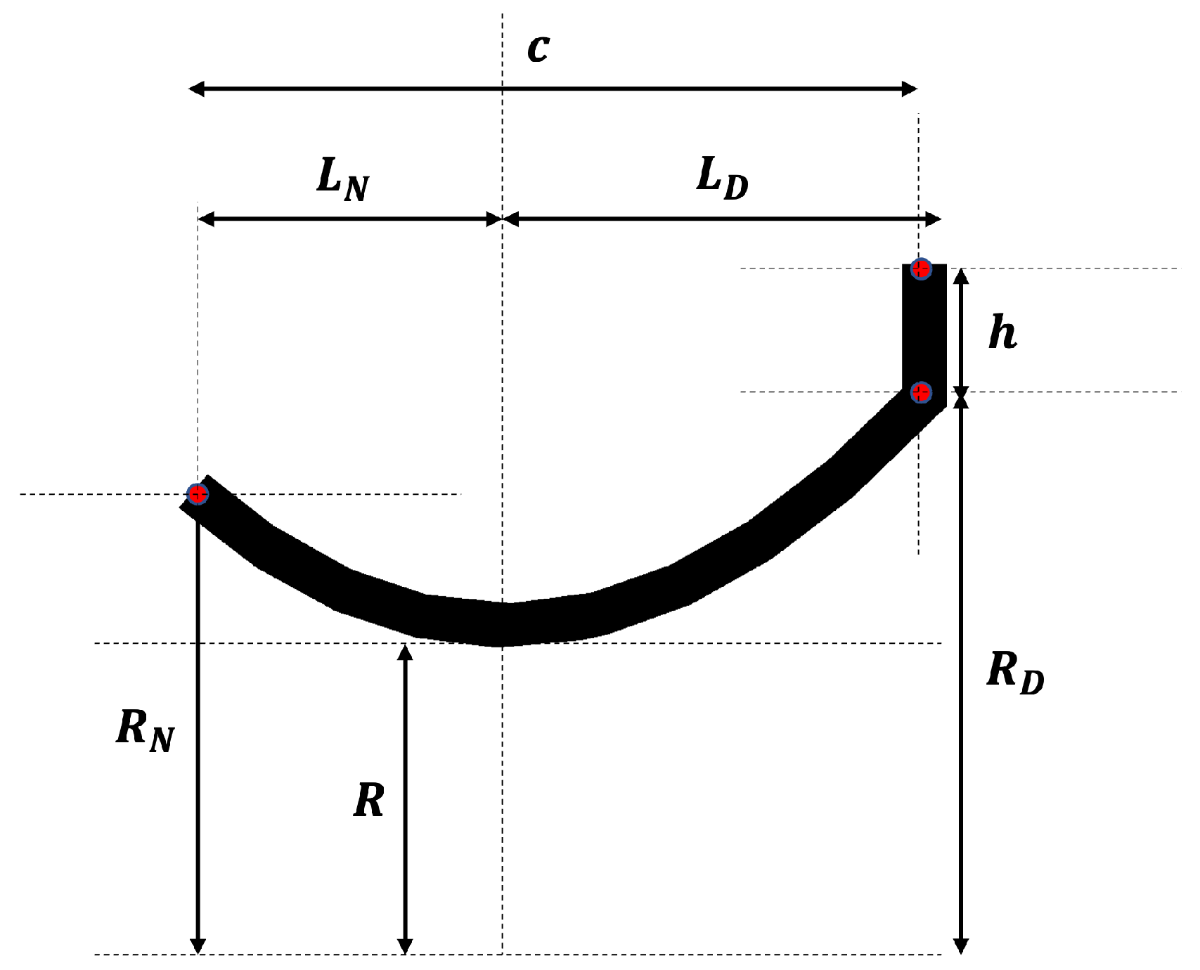
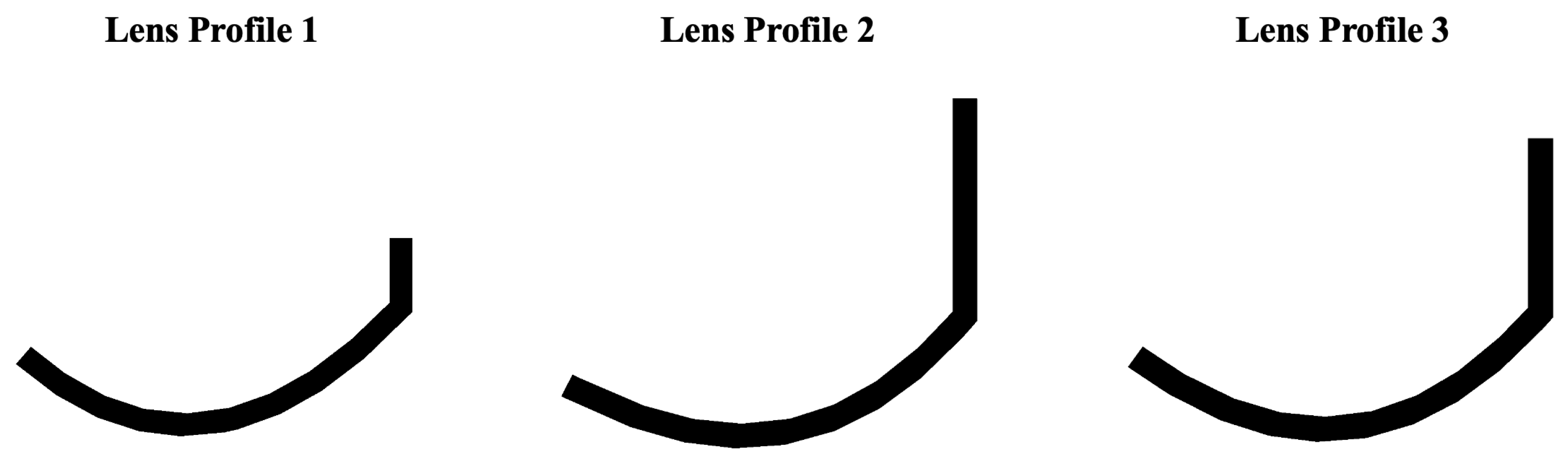
Figure 1. Schematic of a lensed turbine.
Energies 15 04622 g001
Figure 2. Schematic illustrating the aerodynamic interactions between two lensed turbines in a side-by-side arrangement.
Energies 15 04622 g002
Figure 3. Schematic of lensed turbines proximity test in a side-by-side arrangement [13].
Energies 15 04622 g003
Figure 4. Changes in coefficient of power of lensed turbines at close proximities [13].
Energies 15 04622 g004
Figure 5. Geometric features of a wind lens profile.
Energies 15 04622 g005
Figure 6. Three different wind lens profiles (Profile 1, Profile 2, and Profile 3) used in the present study.
Energies 15 04622 g006
Figure 7. Location of PIV field of view behind two identical lens profiles.
Energies 15 04622 g007
Figure 8. Hot-wire grid locations in the wake of two identical lens profiles.
Energies 15 04622 g008
Figure 9. Normalized mean U velocity contours in the wake of three different wind lens profiles.
Energies 15 04622 g009
Figure 10. Normalized mean U vorticity contours in the wake of three different wind lens profiles.
Energies 15 04622 g010
Figure 11. Two-point correlations of V velocity component for all three wind lens profiles at various x / D spacing.
Energies 15 04622 g011
Figure 12. Relative energy of POD modes in the wake of lens profiles 1, 2, and 3.
Energies 15 04622 g012
Figure 13. First four dominant POD modes in the wake of profiles 1, 2, and 3 at various x / D spacing.
Energies 15 04622 g013
Figure 14. POD mode 1 contours in the wake of profiles 1, 2, and 3 wind lenses.
Energies 15 04622 g014
Figure 15. POD mode 2 contours in the wake of profiles 1, 2, and 3 wind lenses.
Energies 15 04622 g015
Figure 16. Wake turbulent intensity results from hot-wire at different downstream locations in the wake of wind lens profiles.
Energies 15 04622 g016
Figure 17. Frequency spectrum highlighting the dominant frequencies at 3 y/c downstream distance from the wind lens pairs.
Energies 15 04622 g017
Table 1. Geometric specifications of three different wind lens profiles.
Lens Profile L D /ch/c R N /c L N /c R D /c C P C D
Profile 10.5740.2501.7050.4261.8240.8960.664
Profile 20.5330.5471.5390.4671.7021.0561.055
Profile 30.5230.4361.5090.4771.6691.0030.876
Publisher’s Note: MDPI stays neutral with regard to jurisdictional claims in published maps and institutional affiliations.

