The Impact of Jumps and Leverage in Forecasting the Co-Volatility of Oil and Gold Futures

Abstract

This paper investigates the impact of jumps in forecasting co-volatility in the presence of leverage effects for daily crude oil and gold futures. We use a modified version of the jump-robust covariance estimator of Koike (2016), such that the estimated matrix is positive definite. Using this approach, we can disentangle the estimates of the integrated co-volatility matrix and jump variations from the quadratic covariation matrix. Empirical results show that more than 80% of the co-volatility of the two futures contains jump variations and that they have significant impacts on future co-volatility but that the impact is negligible in forecasting weekly and monthly horizons.

1. Introduction

The severity and global nature of the recent financial crisis highlighted the risks associated with portfolios containing only conventional financial market assets [1]. Such a realization triggered an interest in considering investment opportunities in the energy (specifically oil) market [2]. In fact, the recent financialization of the commodity market [3,4] and, in particular, oil has resulted in an increased participation of hedge funds, pension funds, and insurance companies in the market, with investment in oil now being considered as a profitable alternative instrument in the portfolio decisions of financial institutions [5,6].

With gold traditionally considered as the most popular ‘safe haven’ [7,8,9], recent studies have analyzed volatility spillovers across the gold and oil markets [10,11,12], where volatility spillovers are defined as the delayed effect of a returns shock in one asset on the subsequent volatility or co-volatility in another asset [13]. For corresponding studies on co-movements in gold and oil returns, see References [14,15,16,17], and references cited therein. A literature review on return and volatility spillovers across asset classes can be found in Reference [18].

In this regard, it must be realized that modelling and forecasting the co-volatility of gold and oil markets is of paramount importance to international investors and portfolio managers in devising optimal portfolio and dynamic hedging strategies [19]. By definition, (partial) co-volatility spillovers occur when the returns shock from financial asset k affects the co-volatility between two financial assets, i and j, one of which can be asset k [13].

Against this backdrop, the objective of this paper is to forecast the daily co-volatility of gold and oil futures derived from 1-min intraday data over the period 27 September 2009 to 25 May 2017 (Although the variability of daily gold and oil price returns have traditionally been forecasted based on Generalized Autoregressive Conditional Heteroskedasticity (GARCH)-type models of volatility, recent empirical evidence suggests that the rich information contained in intraday data can produce more accurate estimates and forecasts of daily volatility (see Reference [20] for a detailed discussion)). In particular, realizing the importance of jumps, that is, discontinuities, in governing the volatility of asset prices [21,22,23], we investigate the impact of jumps by simultaneously accommodating leverage effects in forecasting the co-volatility of gold and oil markets, following the econometric approach of [24] (applied to three stocks traded on the New York Stock Exchange (NYSE)).

Although studies dealing with forecasting gold and oil market volatility has emphasized the role of jumps in forecasting realized volatility. (For a givenfixed interval, realized volatility is defined as the sum of non-overlapping squared returns of high frequency within a day [25] which, in turn, presents volatility as an observed rather than a latent process.) (see, for example, References [26,27,28]), this paper would be seen to be the first attempt to incorporate their role in predicting the future co-volatility path of these two important commodities.

The remainder of the paper is structured as follows—Section 2 lays out the theoretical details of the econometric framework, while Section 3 presents the data, empirical results and analysis. Section 4 gives some concluding remarks.

2. Model Specification

Let $X_{\tau }^{\ast }$ and $Y_{\tau }^{\ast }$ denote latent log-prices at time s for two assets X and Y. Define $p^{\ast }(\tau )={(X_{\tau }^{\ast },Y_{\tau }^{\ast })}^{\prime }$, and let $W(\tau )$ and $Q(\tau )$ denote bivariate vectors of independent Brownian motions and counting processes, respectively. Let $K(\tau )$ be the $2\times 2$ process controlling the magnitude and transmission of jumps, such that $K(\tau )dQ(\tau )$ is the contribution of the jump process to the price diffusion. Under the assumption of a Brownian semimartingale with finite-activity jumps (BSMFAJ), $p^{\ast }(\tau )$ follows:

$$d{p}^{\ast }(\tau )=\mu (\tau )ds+\sigma (\tau )dW(\tau )+K(\tau )dQ(\tau ),0\le \tau \le T$$

(1)

where $\mu (\tau )$ is a $2\times 1$ vector of continuous and locally-bounded variation processes, and $\sigma (\tau )$ is the $2\times 2$ càdlàg matrix, such that $\Sigma (\tau )=\sigma (\tau ){\sigma }^{\prime }(\tau )$ is positive definite. Note that although we explain the framework with finite-activity jumps, the estimators used in this paper are applicable under infinite-activity jumps, as shown by Reference [29].

Assume that the observable log-price process is the sum of the latent log-price process in Equation (1) and the microstructure noise process. Denote the log-price process as $p(\tau )={(X_{\tau },Y_{\tau })}^{\prime }$. Consider non-synchronized trading times of the two assets and let $\mathcal{Z}$ and $\Xi$ be the set of transaction times of X and Y, respectively. Denote the counting process governing the number of observations traded in assets X and Y up to time T as $n_T$ and $m_T$, respectively. By definition, the trades in X and Y occur at times $\mathcal{Z}=\{{\zeta }_1,{\zeta }_2,\dots ,{\zeta }_{n_T}\}$ and $\Xi =\{{\xi }_1,{\xi }_2,\dots ,{\xi }_{m_T}\}$, respectively. For convenience, we set the opening and closing times as ${\zeta }_1={\xi }_1=0$ and ${\zeta }_{n_T}={\xi }_{m_T}=T$, respectively.

The observable log-price process is given by:

$$X_{{\zeta }_i}=X_{{\zeta }_i}^{\ast }+{\epsilon }_{{\zeta }_i}^X\mathrm{and}{Y}_{{\xi }_j}=Y_{{\xi }_j}^{\ast }+{\epsilon }_{{\xi }_j}^Y,$$

(2)

where ${\epsilon }^X\sim \mathrm{iid}(0,{\sigma }_{\epsilon X}^2)$, ${\epsilon }^Y\sim \mathrm{iid}(0,{\sigma }_{\epsilon Y}^2)$, and $({\epsilon }^X,{\epsilon }^Y)$ are independent of $(X,Y)$.

Define the quadratic covariation (QCov) of the log-price process over $[0,T]$ as:

$$\mathrm{QCov}=\underset{\Delta \to \infty }{\mathrm{plim}}\sum _{i=1}^{\lfloor T/\Delta \rfloor }\left[p(i\Delta )-p((i-1)\Delta )\right]{\left[p(i\Delta )-p((i-1)\Delta )\right]}^{\prime }.$$

(3)

By Proposition 2 of Reference [26], we obtain:

$$\mathrm{QCov}=\mathrm{ICov}+\sum _{0<\tau \le T}K(\tau )K^{\prime }(\tau ),$$

(4)

where

$$\mathrm{ICov}={\int }_0^T\Sigma (\tau )d\tau .$$

The first term on the right-hand side of (4) is the integrated co-volatility matrix over $[0,T]$, while the second term is the matrix of jump variability. We are interested in disentangling these two components from the estimates of QCov for the purpose of forecasting QCov.

There are several estimators for QCov and Icov (see the survey in Reference [24]). Among them, we use the estimators of [30] for QCov and [29] for ICov, respectively. Especially, the estimator of Reference [29] is consistent under non-synchronized trading times, jumps and microstructure noise for the bivariate process in (2) (see Appendix A for the detailed explanation of the calculation of these estimators). Note that the realized kernel (RK) estimator of Reference [31] is positive (semi-)definite and robust to microstructure noise under non-synchronized trading times. However, the robustness to jumps is still an open and unresolved issue for the multivariate RK estimator. Denote the estimators of QCov, ICov and jump component at day t as ${\widehat{\Sigma }}_t$, ${\widehat{C}}_t$ and ${\widehat{J}}_t$, respectively, where ${\widehat{J}}_t={\widehat{\Sigma }}_t-{\widehat{C}}_t$ (Jump variations can be defined strictly, as discussed in Reference [32]). By the definitions in (1)–(4), the estimators should be positive (semi-) definite, but there is no guarantee for it. For this purpose, Reference [24] suggest regularizing the estimated covariance matrix by the use of thresholding.

As shown by References [33,34,35], the regularized estimator has consistency, assuming a sparsity structure. Define the thresholding operator for a square matrix A as:

$${\mathcal{T}}_h(A)=[a_{ij}\mathbf{1}(|a_{ij}|\ge h)],$$

(5)

which can be regarded as A thresholded at h. Define the Frobenius norm by ${\left|\right|A\left|\right|}_F^2=tr(A{A}^{\prime })$. For the selection of h, we follow Reference [34]. In order to obtain $\tilde{A}={\mathcal{T}}_h(\widehat{A})$, we minimize the distance by the Frobenius norm $\left|\right|{\mathcal{T}}_h(\widehat{A})-\widehat{A}{\left|\right|}_F^2$, with the restriction that $\tilde{A}$ is positive semi-definite. As in Reference [24], we obtain ${\tilde{C}}_t={\mathcal{T}}_h({\widehat{C}}_t)$ and ${\tilde{J}}_t={\mathcal{T}}_h({\widehat{J}}_t)$, which are consistent and positive semi-definite. Note that ${\widehat{\Sigma }}_t$ is positive semi-definite as it is the sample analogue of QCov. In addition, we also disentangling observed return series into continuous and jump components, by applying the technique of Reference [36] (see Appendix A.3).

In order to examine the effects of jump and leverage in forecasting co-volatility, we consider four kinds of specifications, including the three models introduced by Reference [24]. Let ${\tilde{\Sigma }}_{t(l)}$ denote the l-horizon average, defined by:

$${\tilde{\Sigma }}_{t(l)}=\frac{1}{l}\left({\tilde{\Sigma }}_t+\cdots +{\tilde{\Sigma }}_{t-l+1}\right).$$

In order to examine the impact of jumps and leverage for forecasting volatility and co-volatility, we use four kinds of heterogeneous autoregressive (HAR) models for forecasting the ($i,j$)-elements of ${\tilde{\Sigma }}_{t(l)}$$(l=1,5,22)$, as follows:

$$\begin{array}{cc}\hfill & {\tilde{\Sigma }}_{ij,t(l)}={\gamma }_0+{\gamma }_d{\tilde{\Sigma }}_{ij,t-1}+{\gamma }_w{\tilde{\Sigma }}_{ij,t-1(5)}+{\gamma }_m{\tilde{\Sigma }}_{ij,t-1(22)}+e_{ij,t}\hfill \end{array}$$

(6)

$$\begin{array}{cc}\hfill & {\tilde{\Sigma }}_{ij,t(l)}={\gamma }_0+{\gamma }_d{\tilde{\Sigma }}_{ij,t-1}+{\gamma }_w{\tilde{\Sigma }}_{ij,t-1(5)}+{\gamma }_m{\tilde{\Sigma }}_{ij,t-1(22)}+{\gamma }_a{r}_{i,t-1}^{-}{r}_{j,t-1}^{-}+e_{ij,t}\hfill \end{array}$$

(7)

$$\begin{array}{cc}\hfill & {\tilde{\Sigma }}_{ij,t(l)}={\gamma }_0+{\gamma }_d{\tilde{C}}_{ij,t-1}+{\gamma }_w{\tilde{C}}_{ij,t-1(5)}+{\gamma }_m{\tilde{C}}_{ij,t-1(22)}+{\gamma }_j{\tilde{J}}_{ij,t-1}+e_{ij,t}\hfill \end{array}$$

(8)

$$\begin{array}{cc}\hfill & {\tilde{\Sigma }}_{ij,t(l)}={\gamma }_0+{\gamma }_d{\tilde{C}}_{ij,t-1}+{\gamma }_w{\tilde{C}}_{ij,t-1(5)}+{\gamma }_m{\tilde{C}}_{ij,t-1(22)}+{\gamma }_j{\tilde{J}}_{ij,t-1}+{\gamma }_{a}r{c}_{i,t-1}^{-}r{c}_{j,t-1}^{-}+e_{ij,t},\hfill \end{array}$$

(9)

where $r_{i,t}^{-}=r_{i,t}I(r_{i,t}<0)$ and $r{c}_{i,t}^{-}=r{c}_{i,t}I(r{c}_{i,t}<0)$, which are the negative parts of the observed return and its continuous part for the i-th asset. The second model accommodates the asymmetric effects, as in the specification of the asymmetric BEKK model of Reference [37]. For $i\ne j$, ${\gamma }_a{r}_{i,t-1}^{-}{r}_{j,t-1}^{-}$ represents the ‘co-leverage’ effect, which is caused by simultaneous negative returns in two assets. In the third model, we use the previous values of the estimated continuous sample path component variation, ${\tilde{C}}_t$, rather than those of the estimated quadratic variation, ${\tilde{\Sigma }}_t$, following the volatility forecasting models of References [21,23]. We exclude weekly and monthly effects of the jump component, ${\tilde{J}}_t$, in order to evaluate the impact of a single jump on future volatility and co-volatility. Note that ${\tilde{C}}_t$ and ${\tilde{J}}_t$ are positive (semi-) definite by the thresholding in (5). In addition to jump variability, the fourth model includes the asymmetric effect. Note that we use the continuous components of returns rather than the observed returns for the fourth model. We refer to Equations (6)–(9) as the HAR, HAR-A, HAR-TCJ and HAR-TCJA models, respectively. We estimate these models by ordinary least squares (OLS) and use the heteroskedasticity and autocorrelation consistent (HAC) covariance matrix estimator, with bandwidth 25 (see Reference [38]). We will examine the four models (6)–(9) in the next section.

3. Empirical Analysis

We examine the effects on jumps and leverage in forecasting co-volatility, using the estimates of QCov, ICov and jump variation, for two futures contracts traded on the New York Mercantile Exchange (NYMEX), namely West Texas Intermediate (WTI) Crude Oil and Gold. With the CME Globex system, the trades at NYMESX cover 24 h (The futures price data, in continuous format, are obtained from http://www.kibot.com/). Based on the vector of returns for the two futures for a 1-min interval of trading day at t, we calculated the daily values of ${\tilde{\Sigma }}_t$, ${\tilde{C}}_t$ and ${\tilde{J}}_t$, as explained in the previous section and also the corresponding open-close returns and their continuous components, $r_t$ and $r{c}_t$, respectively, for the two futures. The sample period starts on 27 September 2009 and ends on 25 May 2017, giving 1978 observations. The sample is divided into two periods—the first 1000 observations are used for in-sample estimation, while the last 978 observations are used for evaluating the out-of-sample forecasts.

Table 1. Descriptive statistics of returns, volatility and co-volatility.

Stock	Mean	Std. Dev.	Skew.	Kurt.	Jump
Return
Crude Oil	0.0256	0.6824	−0.4784	8.0378	0.9267
Gold	0.0185	1.4887	−0.0573	5.0225	0.9459
Volatility
Crude Oil	0.4238	0.5070	7.2211	90.688	0.9267
Gold	1.5152	1.6510	3.3689	19.071	0.9459
Co-Volatility
(Crude Oil, Gold)	0.1368	0.2844	−0.7851	37.359	0.8049

Note: The sample period is from 27 September 2009 to 25 May 2017. ‘Jump’ denotes the percentage of occurrence of significant jumps.

presents the descriptive statistics of the returns, $r_t$, and estimated QCov, ${\tilde{\Sigma }}_t$. The empirical distribution of the returns is highly leptokurtic. Regarding volatility, their distributions are skewed to the right, with evidence of heavy tails in the two series. More than 90% of the sample period contains significant jumps in volatility. For co-volatility, the empirical distribution is highly leptokurtic and co-jump variations were found for 80% of the period.

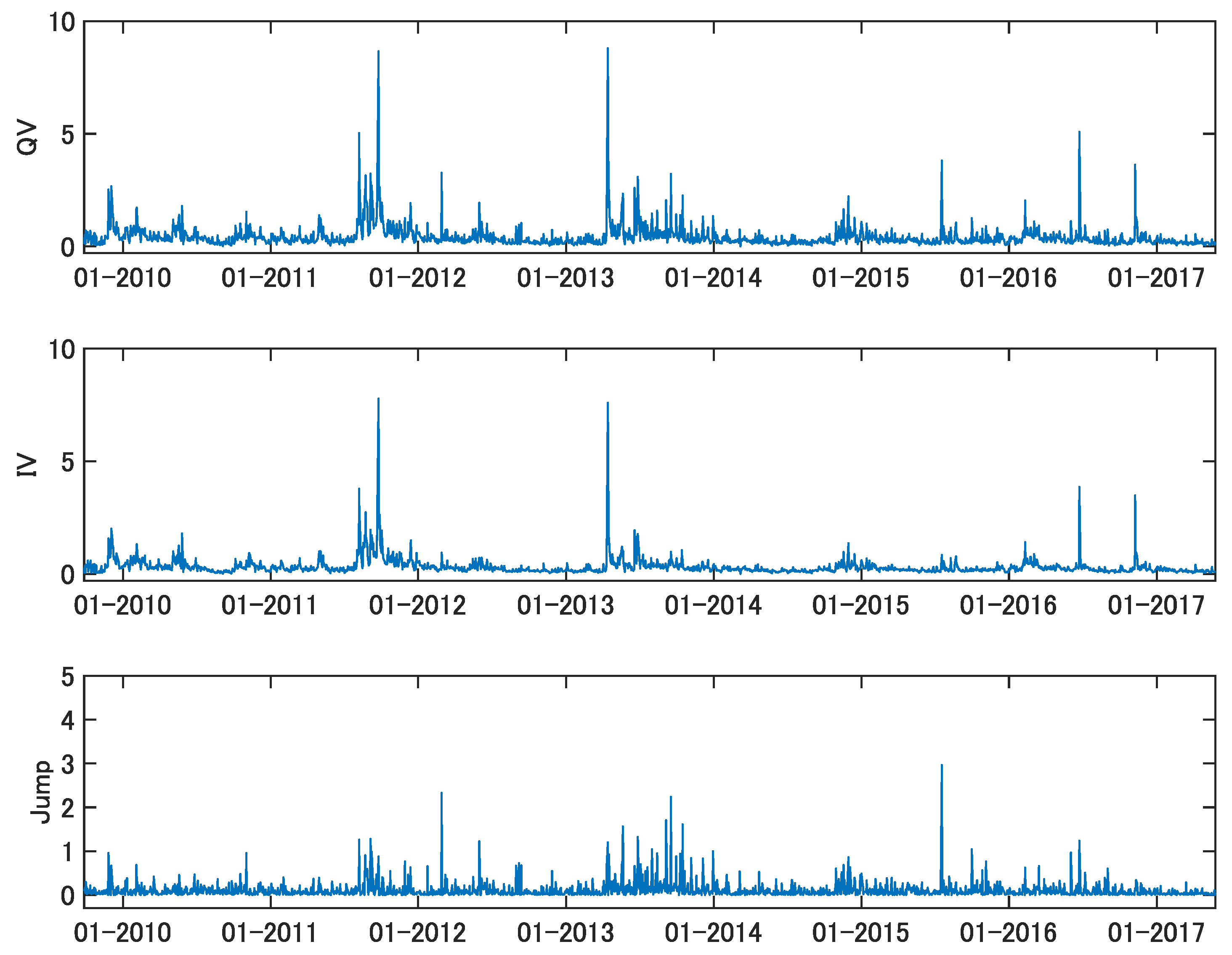
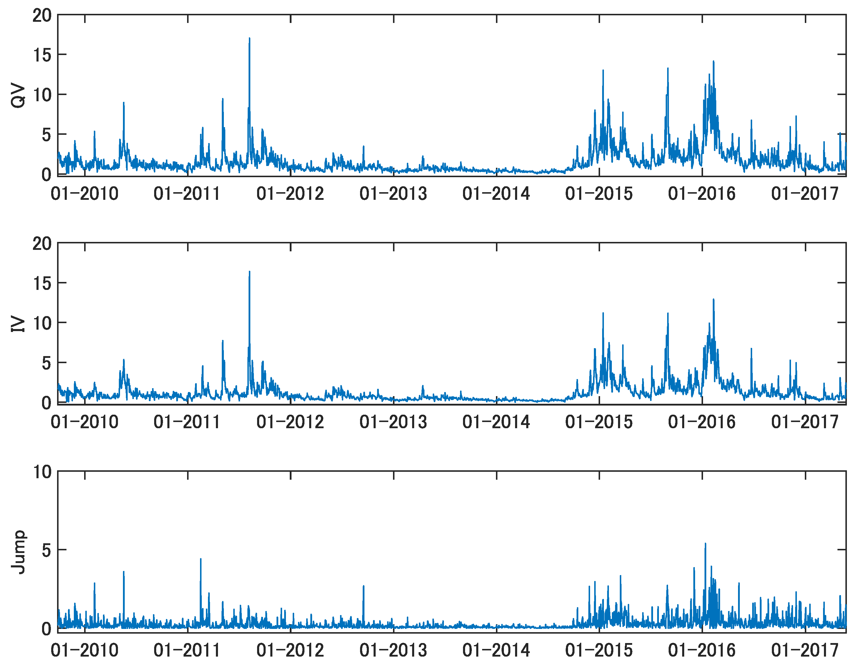
Figure 1 and Figure 2 show the estimates of quadratic variation, integrated volatility, and jump variability, namely the diagonal elements of ${\tilde{\Sigma }}_t$, ${\tilde{C}}_t$, and ${\tilde{J}}_t$, respectively. It is known that spot and future prices of crude oil are effected by a variety of geopolitical and economic events. For instance, the estimates of volatility in Figure 1 are relatively high for the period following the Arab Spring of 2011, and the extreme jump in 2015 is caused by the oversupply and the technological advancements of US shale oil production. On the other hand, the spot and futures prices of Gold reflect news and recessions, as investigated by Reference [39]. The estimates of volatility are high in 2011 during the European debt crisis, and the last one-third in Figure 2. For the latter, it corresponds to China’s economy growing at its slowest pace for 24 years in 2014.

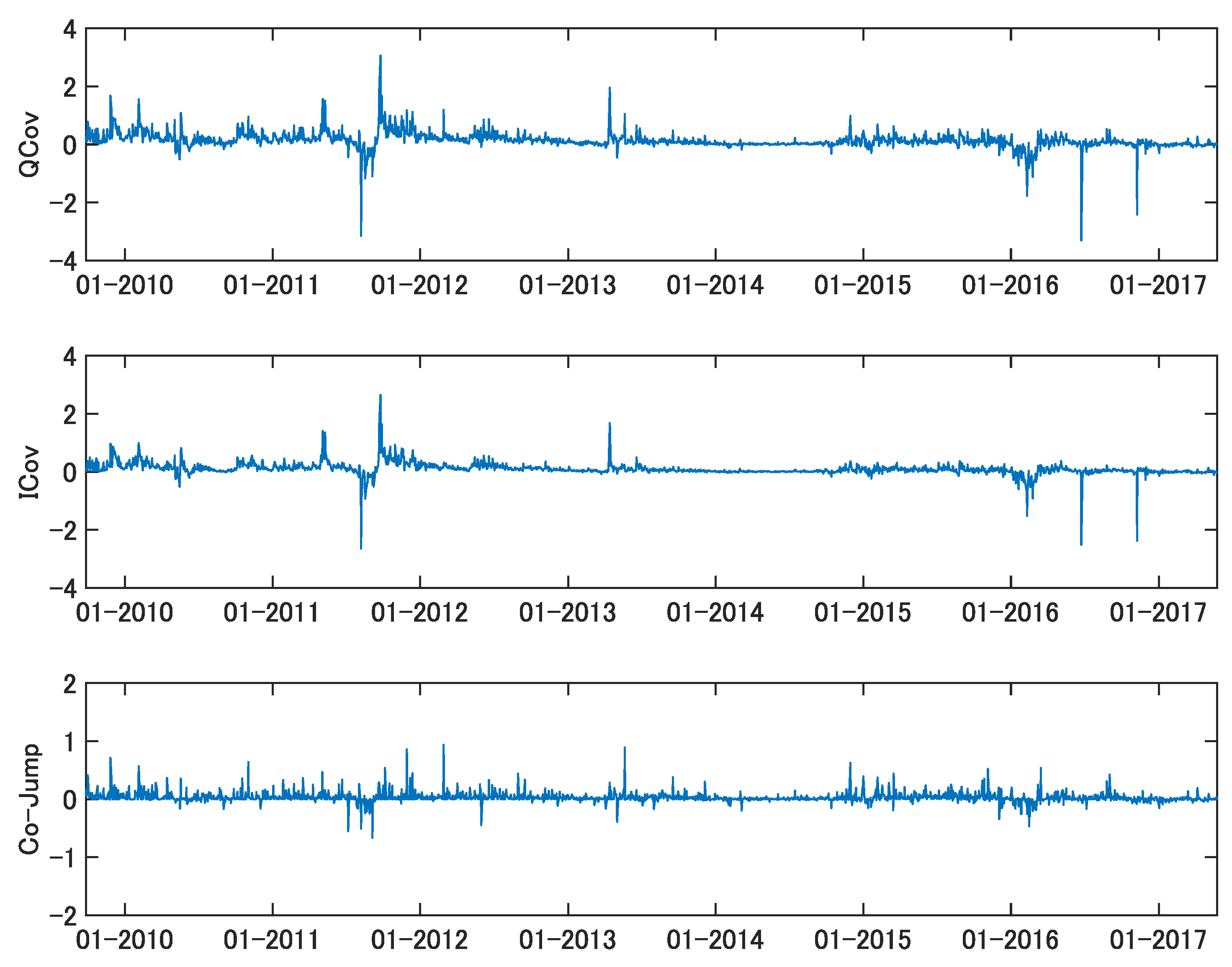
Figure 3 illustrates the estimates of quadratic covariation, integrated co-volatility and jump co-variability, namely the $(2,1)$-element of ${\tilde{\Sigma }}_t$, ${\tilde{C}}_t$, and ${\tilde{J}}_t$. Figure 3 indicates that crude oil and gold futures are negatively correlated for the first half in 2011, but the sign changes for the latter half. A large and positive co-jump variability is found in 2013, which reflects the political unrest in Egypt and the values of Dow Jones Industrial Average kept increasing with a rapid trend.

In the following empirical analysis based on the four models (6)–(9), we:

(a)

examine the robustness of the positive effects of jump components under microstructure noise for the volatility equation ($i=j$);

(b)

test the robustness of the leverage effects under jump and microstructure noise for the volatility equation;

(c)

investigate the effects of co-jumps and co-leverage for the co-volatility equation;

(d)

compare the out-of-sample forecasts of the above models.

For the above models for the volatility equation, the estimates of ${\gamma }_j$ are expected to be positive. However, the empirical results of Reference [21] indicate that the estimates of ${\gamma }_j$ are generally insignificant. Reference [23] noted that the puzzle is due to the small sample bias of the integrated volatility, and found that the estimates of ${\gamma }_j$ are positive and significant. Since the estimators of quadratic variation and integrated volatility used in Reference [23] are biased in the presence of microstructure noise, we re-examine the robustness of the result and this is the motivation of (a). With respect to (b), we also test ${\gamma }_a>0$ under microstructure noise in order to check the robustness of the result of Reference [40]. Among (a)–(d), (c) is the main purpose of the current empirical analysis.

For volatility equation ($i=j$), the estimates of ${\gamma }_j$ and ${\gamma }_a$ are expected to be positive and significant. On the other hand, their signs are not determined for the co-volatility equation ($i\ne j$). As noted in (d), we compare the forecasting performances of the HAR, HAR-TCJ and HAR-TCJA models for daily, weekly and monthly horizons. For crude oil futures, Reference [41] found that HAR-TCJA is the best forecasting one-day-ahead volatility, while the HAR model is preferred for weekly and monthly forecasts, after removing the effects of structural breaks. In addition to crude oil, we examine the forecasting performances of the volatility of gold futures and the co-volatility of the two futures.

As stated in the previous section, we use the HAC estimator for the covariance matrix of the OLS estimators. To ensure the statistical adequacy of the approach, we conduct three kinds of conventional diagnostic tests. The first is the White test for heteroskedasticity. When the number of explanatory variables is k, excluding the constant, the Wald statistic for the White test has the asymptotic ${\chi }^2$ distribution with the degree-of-freedom parameter $(k+1)(k+2)/2$ under the null of homoskedasticity. The second test is the ARCH(2) test with the auxiliary regression:

$${\widehat{e}}_{ij,t}^2={\delta }_0+{\delta }_1{\widehat{e}}_{ij,t-1}^2+{\delta }_2{\widehat{e}}_{ij,t-1}^2+{error}_{ij,t},$$

where ${\widehat{e}}_{ij,t}$ is the residuals. Under the null hypothesis of homoskedasticity, that is ${\delta }_1={\delta }_2=0$, the Wald statistic has the asymptotic ${\chi }^2$ distribution with the degree-of-freedom parameter 2. The third one is the test for autocorrelation with the auxiliary regression:

$${\widehat{e}}_{ij,t}={\rho }_0+{\rho }_1{\widehat{e}}_{ij,t-1}+\cdots +{\rho }_{10}{\widehat{e}}_{ij,t-1}+{error}_{ij,t}.$$

Under the null hypothesis of no autocorrelation, that is ${\rho }_1=\cdots ={\rho }_{10}=0$, the Wald statistic has the asymptotic ${\chi }^2$ distribution with the degree-of-freedom parameter 10.

We estimate each model using the first 1000 observations, and obtain a forecast, ${\tilde{\Sigma }}_{1001}^f$. We re-estimate each model fixing the sample size at 1000, and obtain new forecasts based on updated parameter estimates. For evaluating the forecasting performance of the different models, we consider the Mincer and Zarnowitz (MZ) [42] regression, namely:

$${\tilde{\Sigma }}_{ij,t}={\alpha }_0+{\alpha }_1{\tilde{\Sigma }}_{ij,t}^f+{error}_{ij,t},t=1001,\dots ,1978.$$

We estimate the MZ regression via the OLS and report $R^2$ for comparing forecasting performance. Intuitively, a model with the highest $R^2$ indicates the accuracy of forecasts. We also use the heteroskedasticity-adjusted root mean square error suggested in Reference [43], namely:

$$\mathrm{HRMSE}=\sqrt{\frac{1}{978}{\sum }_{t=1001}^{1978}{\left(\frac{{\tilde{\Sigma }}_{ij,t}-{\tilde{\Sigma }}_{ij,t}^f}{{\tilde{\Sigma }}_{ij,t}}\right)}^2}.$$

For the latter, we examine equal forecast accuracy using the Diebold-Mariano (DM) [44] test at the 5% significance level, and use the HAC covariance matrix estimator, with bandwidth 25. We also examine the forecasts of ${\tilde{\Sigma }}_{ij,t(5)}$ and ${\tilde{\Sigma }}_{ij,t(22)}$ in the same manner.

As an application of forecasts of covariance matrix, we examine performances of portfolio weights determined by the forecasts. We consider a portfolio of two options, $r_{pt}=w_t^{\prime }\{p(t)-p(t-1)\}$, where $p(s)$ is the vector of log-prices stated in Section 2 and $w_t$ is the vector of portfolio weights. With the forecasts of covariance matrix, ${\tilde{\Sigma }}_t^f$, the weights of the minimum variance portfolio are given by:

$$w_t^{\ast }={({\iota }^{\prime }{\tilde{\Sigma }}_t^{f-1}\iota )}^{-1}{\tilde{\Sigma }}_t^{f-1}\iota ,$$

(10)

where $\iota ={(1,1)}^{\prime }$. Given the realized value ${\tilde{\Sigma }}_t$, the corresponding portfolio variance is evaluated as:

$${\sigma }_{pt}^2=w_t^{\ast \prime }{\tilde{\Sigma }}_t{w}_t^{\ast }.$$

(11)

We calculate the HRMSE of ${\sigma }_{pt}^2$ for the four models, and compare the values by the DM test. In the same manner, we compare the portfolio weights of the minimum variance portfolio based on the forecasts of ${\tilde{\Sigma }}_{ij,t(5)}$ and ${\tilde{\Sigma }}_{ij,t(22)}$.

Table 2. In-sample estimates for daily regressions.

Model	${\mathit{\gamma }}_0$	${\mathit{\gamma }}_{\mathit{d}}$	${\mathit{\gamma }}_{\mathit{w}}$	${\mathit{\gamma }}_{\mathit{m}}$	${\mathit{\gamma }}_{\mathit{j}}$	${\mathit{\gamma }}_{\mathit{a}}$	${\mathit{R}}^2$	${\overline{\mathit{R}}}^2$
Volatility: Crude Oil
HAR	0.0958	0.4428	0.1047	0.2665			0.3514	0.3494
	(0.0021)	(0.0054)	(0.0050)	(0.0056)
HAR-A	0.1067	0.2258	0.2000	0.2905		0.1301	0.4153	0.4129 †
	(0.0018)	(0.0039)	(0.0040)	(0.0056)		(0.0032)
HAR-TCJ	0.1239	0.5182	0.1012	0.2879	0.2410		0.3546	0.3520
	(0.0017)	(0.0083)	(0.0064)	(0.0064)	(0.0112)
HAR-TCJA	0.1301	0.2285	0.2431	0.3176	0.2575	0.1292	0.4140	0.4110
	(0.0015)	(0.0067)	(0.0054)	(0.0064)	(0.0097)	(0.0032)
Volatility: Gold
HAR	0.2039	0.4730	0.2067	0.1462			0.4396	0.4378
	(0.0028)	(0.0060)	(0.0053)	(0.0043)
HAR-A	0.0356	0.3161	0.3324	0.1337		0.0574	0.4320	0.4296
	(0.0009)	(0.0045)	(0.0046)	(0.0062)		(0.0010)
HAR-TCJ	0.2520	0.5629	0.1512	0.1767	0.2913		0.4414	0.4391
	(0.0027)	(0.0082)	(0.0057)	(0.0048)	(0.0094)
HAR-TCJA	0.2193	0.4612	0.2066	0.1621	0.2427	0.1189	0.5266	0.5242 †
	(0.0024)	(0.0066)	(0.0051)	(0.0041)	(0.0069)	(0.0014)
Co-Volatility: Crude Oil & Gold
HAR	0.0431	0.3938	0.3199	0.0923			0.4034	0.4016
	(0.0009)	(0.0043)	(0.0049)	(0.0064)
HAR-A	0.1704	0.3793	0.2547	0.1328		0.1205	0.5271	0.5252 †
	(0.0024)	(0.0052)	(0.0048)	(0.0036)		(0.0014)
HAR-TCJ	0.0515	0.5028	0.3268	0.1447	0.2047		0.4116	0.4092
	(0.0008)	(0.0065)	(0.0060)	(0.0071)	(0.0057)
HAR-TCJA	0.0444	0.4086	0.3486	0.1933	0.1664	0.0564	0.4391	0.4362
	(0.0008)	(0.0069)	(0.0057)	(0.0068)	(0.0049)	(0.0010)

Note: Standard errors are given in parentheses. ‘†’ denotes the model which has the highest ${\overline{R}}^2$ value of the four models.

shows the estimates of the daily regressions for the first 1000 observations. For the jump parameter, ${\gamma }_j$, the estimates are positive and significant at five percent level in all cases. The results for the volatilities support the empirical evidence of Reference [23]. For the asymmetric effect, the estimates of ${\gamma }_a$ are positive and significant in all cases, supporting the negative relationship between return and one-step-ahead volatility, as in Reference [40]. The results for the co-volatility equation indicate that a pair of negative returns and/or co-jumps of two assets increases future co-volatility. Either of HAR-A and HAR-TCJA model gives the highest ${\overline{R}}^2$ in all cases.

Table 3. Diagnostic tests for daily regressions.

Model	White	d.f.	p-Value	ARCH(2)	p-Value	AutoCor (10)	p-Value
Volatility: Crude Oil
HAR	68.955	10	[0.0000]	7.3212	[0.0257]	12.849	[0.2322]
HAR-TCJ	137.08	15	[0.0000]	8.6057	[0.0135]	12.510	[0.2524]
HAR-TCJA	565.48	21	[0.0000]	15.150	[0.0005]	18.158	[0.0524]
HAR-A	280.45	15	[0.0000]	14.439	[0.0007]	17.012	[0.0741]
Volatility: Gold
HAR	127.72	10	[0.0000]	58.588	[0.0007]	28.195	[0.0017]
HAR-TCJ	162.06	15	[0.0000]	66.637	[0.0000]	27.113	[0.0025]
HAR-TCJA	369.97	21	[0.0000]	27.265	[0.0000]	29.001	[0.0013]
HAR-A	284.90	15	[0.0000]	22.363	[0.0000]	30.453	[0.0007]
Co-Volatility: Crude Oil & Gold
HAR	62.977	10	[0.0000]	25.708	[0.0000]	9.5972	[0.4765]
HAR-TCJ	74.695	15	[0.0000]	30.078	[0.0000]	9.6906	[0.4680]
HAR-TCJA	87.284	21	[0.0000]	17.846	[0.0000]	12.637	[0.2447]
HAR-A	67.424	15	[0.0000]	14.547	[0.0000]	15.075	[0.1294]

Note: The table presents the values of the diagnostic statistics for the OLS residuals. ‘White’ denotes the White test for heteroskedasticity, ‘ARCH(2)’ is the ARCH(2) test, and AutoCorr(10)’ is the test for 10th-order autocorrelation. ‘df‘ denotes the degree-of-freedom. While the ARCH(2) test has the asymptotic ${\chi }^2(2)$ under the null hypothesis, the asymptotic distribution of AutoCorr(10) test is ${\chi }^2(10)$.

presents the diagnostic statistics for the daily regressions. White and ARCH(2) reject the null hypothesis of homoskedasticity at the five percent level in all cases. The test for 10th-order autocorrelation rejected the null hypothesis of no autocorrelation for the volatility of Gold futures. Hence, it is justified to use the HAC covariance matrix estimates for the OLS estimates in Table 2. The corresponding results for the weekly and monthly regressions are omitted to save space.

Table 4. Out-of-sample forecast evaluation for daily regressions.

Model	${\mathit{R}}^2$	HRMSE	${\mathit{R}}^2$-J	HRMSE-J	${\mathit{R}}^2$-C	HRMSE-C
Volatility: Crude Oil (900 Times Jump)
HAR	0.0796	2.5591	0.0818	2.6478	0.0590	1.1057
HAR-A	0.0987	2.0655	0.1023	2.1329	0.0702	1.0018
HAR-TCJ	0.0928	2.0476	0.0944	2.1156	0.0775 †	0.9635
HAR-TCJA	0.0995 †	2.0205	0.1037 †	2.0869	0.0641	0.9672
Volatility: Gold (950 Times Jump)
HAR	0.6900	0.9009	0.6918	0.9066	0.6017	0.7857
HAR-A	0.6933 †	0.8376	0.6944 †	0.8431	0.6292 †	0.7249
HAR-TCJ	0.6907	0.9103	0.6929	0.9132	0.5891	0.8534
HAR-TCJA	0.6925	0.8493	0.6938	0.8521	0.6211	0.7945
Co-Volatility: Crude Oil & Gold (616 Times Co-Jump)
HAR	0.2199 †	40.906	0.1897	45.317	0.3247 †	32.033
HAR-A	0.2197	41.743	0.2007 †	45.906	0.2927	33.489
HAR-TCJ	0.2103	36.572	0.1832	40.316	0.3127	29.114
HAR-TCJA	0.2119	37.543	0.1971	41.018	0.2806	30.739

Note: The table presents $R^2$ for the MZ regression and heteroskedasticity-adjusted root mean squared error (HRMSE). $R^2$-J (HRMSE-J) is $R^2$ (HRMSE) conditionally on having a jump at time $t-1$, respectively, while $R^2$-C (HRMSE-C) is conditional on no jump at time $t-1$. ‘†’ indicates the model which has the highest $R^2$ value of the four models. For the DM test of equal forecast accuracy, there were no significant differences at the five percent level.

presents $R^2$ of the MZ regressions and HRMSE for the daily regressions. The HAR-A has the highest $R^2$ for four-ninth of the cases, while the results of the DM tests regarding the HRMSE indicate that there are no significant differences for the four models in all cases.

Table 5. In-sample estimates for weekly regressions.

Model	${\mathit{\gamma }}_0$	${\mathit{\gamma }}_{\mathit{d}}$	${\mathit{\gamma }}_{\mathit{w}}$	${\mathit{\gamma }}_{\mathit{m}}$	${\mathit{\gamma }}_{\mathit{j}}$	${\mathit{\gamma }}_{\mathit{a}}$	${\mathit{R}}^2$	${\overline{\mathit{R}}}^2$
Volatility: Crude Oil
HAR	0.0203	0.1731	0.7803	0.0070			0.9208	0.9206
	(0.0006)	(0.0015)	(0.0028)	(0.0017)
HAR-A	0.0221	0.1387	0.7954	0.0108		0.0206	0.9237	0.9234 †
	(0.0005)	(0.0015)	(0.0029)	(0.0017)		(0.0008)
HAR-TCJ	0.0562	0.1843	0.8853	0.0002	0.2655		0.9060	0.9057
	(0.0006)	(0.0024)	(0.0039)	(0.0022)	(0.0028)
HAR-TCJA	0.0571	0.1441	0.9050	0.0043	0.2678	0.0179	0.9081	0.9076
	(0.0006)	(0.0026)	(0.0039)	(0.0023)	(0.0026)	(0.0008)
Volatility: Gold
HAR	0.0446	0.1793	0.7970	−0.0142			0.9403	0.9402
	(0.0008)	(0.0016)	(0.0023)	(0.0012)
HAR-A	0.0380	0.1609	0.8064	−0.0168		0.0236	0.9456	0.9454 †
	(0.0007)	(0.0015)	(0.0023)	(0.0012)		(0.0003)
HAR-TCJ	0.1086	0.2244	0.8310	−0.0058	0.2440		0.9240	0.9237
	(0.0009)	(0.0023)	(0.0033)	(0.0016)	(0.0019)
HAR-TCJA	0.1027	0.2059	0.8411	−0.0084	0.2351	0.0217	0.9285	0.9281
	(0.0009)	(0.0021)	(0.0033)	(0.0016)	(0.0015)	(0.0003)
Co-Volatility: Crude Oil & Gold
HAR	0.0099	0.1441	0.8321	−0.0207			0.9346	0.9344
	(0.0002)	(0.0012)	(0.0020)	(0.0017)
HAR-A	0.0084	0.1277	0.8347	−0.0120		0.0121	0.9367	0.9364 †
	0.0002)	(0.0012)	(0.0020)	(0.0016)		(0.0002)
HAR-TCJ	0.0237	0.1790	0.9493	0.0140	0.1996		0.9160	0.9157
	(0.0003)	(0.0021)	(0.0031)	(0.0024)	(0.0013)
HAR-TCJA	0.0222	0.1594	0.9538	0.0241	0.1916	0.0117	0.9180	0.9176
	(0.0003)	(0.0022)	(0.0031)	(0.0023)	(0.0011)	(0.0003)

Note: Standard errors are given in parentheses.‘†’ denotes the model which has the highest ${\overline{R}}^2$ value of the four models.

reports the estimates of the weekly regressions. The estimates of the jump parameter, ${\gamma }_j$, and the parameter of the asymmetric effect, ${\gamma }_a$, are positive and significant. For the weekly regressions, the HAR-A model gives the highest ${\overline{R}}^2$ values in all cases.

Table 6. Out-of-sample forecast evaluation for weekly regressions.

Model	MZ ${\mathit{R}}^2$	HRMSE	${\mathit{R}}^2$-J	HRMSE-J	${\mathit{R}}^2$-C	HRMSE-C
Volatility: Crude Oil (900 Times Jump)
HAR	0.8060	0.1980 c,d	0.7964	0.2011 c,d	0.8792	0.1578 c,d
HAR-A	0.8138 †	0.1996 c,d	0.8035 †	0.2032 c,d	0.8874 †	0.1523 c,d
HAR-TCJ	0.7321	0.2444	0.7286	0.2469	0.8064	0.2141
HAR-TCJA	0.7381	0.2465	0.7340	0.2492	0.8120	0.2128
Volatility: Gold (929 Times Jump)
HAR	0.9748	0.1258 c,d	0.9750	0.1262 c,d	0.9639	0.1168
HAR-A	0.9755 †	0.1224 a,c,d	0.9756 †	0.1228 a,c,d	0.9679 †	0.1158
HAR-TCJ	0.9692	0.1592	0.9693	0.1595	0.9601	0.1546
HAR-TCJA	0.9697	0.1557 c	0.9698	0.1559 c	0.9647	0.1510
Co-Volatility: Crude Oil & Gold (616 Times Co-Jump)
HAR	0.8884 †	9.2664	0.8695	11.509	0.9138 †	2.5693
HAR-A	0.8876	8.2840	0.8709 †	10.254	0.9102	2.5458
HAR-TCJ	0.8567	4.7787	0.8391	5.0081	0.8834	4.3606
HAR-TCJA	0.8564	4.0257	0.8409	3.9249	0.8799	4.1917

Note: The table presents $R^2$ for the MZ regression and heteroskedasticity-adjusted root mean squared error (HRMSE). $R^2$-J (HRMSE-J) is $R^2$ (HRMSE) conditionally on having a jump at time $t-1$, respectively, while $R^2$-C (HRMSE-C) is conditional on no jump at time $t-1$. ‘†’ indicates the model which has the highest $R^2$ value of the four models. For the DM test of equal forecast accuracy, ‘a’, ‘b’, ‘c’, and ‘d’ denote significant improvements in forecasting performance with respect to the HAR, HAR-A, HAR-TCJ and HAR-TCJA models, respectively.

gives the $R^2$ values of the MZ regressions, and HRMSE for the out-of-sample forecasts for the weekly regressions. Table 5 and Table 6 indicate that the values of $R^2$ (and ${\overline{R}}^2$) are higher than those for the daily regressions in Table 2 and Table 4, respectively. Table 6 shows that the HAR-A model gives the highest ${\overline{R}}^2$ for volatility. For co-volatility, $R^2$ for MZ tends to select the HAR model, while HRMSE chooses the HAR-A model. However, the DM tests show that there are no significant differences for the four models for co-volatility.

Table 7. In-sample estimates for monthly regressions.

Model	${\mathit{\gamma }}_0$	${\mathit{\gamma }}_{\mathit{d}}$	${\mathit{\gamma }}_{\mathit{w}}$	${\mathit{\gamma }}_{\mathit{m}}$	${\mathit{\gamma }}_{\mathit{j}}$	${\mathit{\gamma }}_{\mathit{a}}$	${\mathit{R}}^2$	${\overline{\mathit{R}}}^2$
Volatility: Crude Oil
HAR	0.0010	0.0148	0.0261	0.9573			0.9913	0.9913
	(0.0001)	(0.0003)	(0.0003)	(0.0005)
HAR-A	0.0015	0.0049	0.0305	0.9584		0.0059	0.9917	0.9917 †
	0.0001)	(0.0002)	(0.0003)	(0.0005)		(0.0001)
HAR-TCJ	0.0441	0.0117	0.0430	1.0977	0.0752		0.9741	0.9740
	(0.0003)	(0.0004)	(0.0008)	(0.0016)	(0.0009)
HAR-TCJA	0.0444	−0.0031	0.0503	1.0992	0.0760	0.0066	0.9746	0.9745
	(0.0003)	(0.0003)	(0.0008)	(0.0016)	(0.0008)	(0.0002)
Volatility: Gold
HAR	−0.0017	0.0201	0.0288	0.9518			0.9931	0.9931
	(0.0003)	(0.0003)	(0.0004)	(0.0005)
HAR-A	−0.0033	0.0157	0.0311	0.9511		0.0057	0.9936	0.9936 †
	(0.0003)	(0.0002)	(0.0004)	(0.0005)		(0.0001)
HAR-TCJ	0.0819	0.0198	0.0335	1.0575	0.0850		0.9820	0.9819
	(0.0004)	(0.0005)	(0.0007)	(0.0008)	(0.0008)
HAR-TCJA	0.0805	0.0154	0.0360	1.0569	0.0829	0.0052	0.9824	0.9823
	(0.0004)	(0.0004)	(0.0007)	(0.0008)	(0.0007)	(0.0001)
Co-Volatility: Crude Oil & Gold
HAR	−0.0004	0.0166	0.0363	0.9482			0.9922	0.9922
	(0.0001)	(0.0002)	(0.0003)	(0.0005)
HAR-A	−0.0007	0.0133	0.0369	0.9500		0.0025	0.9924	0.9924 †
	(0.0001)	(0.0002)	(0.0003)	(0.0005)		(0.0001)
HAR-TCJ	0.0184	0.0131	0.0279	1.1670	0.0551		0.9790	0.9790
	(0.0001)	(0.0004)	(0.0006)	(0.0011)	(0.0006)
HAR-TCJA	0.0181	0.0093	0.0288	1.1690	0.0536	0.0023	0.9792	0.9791
	(0.0001)	(0.0004)	(0.0006)	(0.0011)	(0.0006)	(0.0001)

Note: Standard errors are given in parentheses. ‘†’ denotes the model which has the highest ${\overline{R}}^2$ value of the four models.

shows the in-sample estimates of the monthly regressions, while

Table 8. Out-of-sample forecast evaluation for monthly regressions.

Model	MZ ${\mathit{R}}^2$	HRMSE	${\mathit{R}}^2$-J	HRMSE-J	${\mathit{R}}^2$-C	HRMSE-C
Volatility: Crude Oil (900 Times Jump)
HAR	0.9794	0.0542 c,d	0.9786	0.0552 c,d	0.9856	0.0424 c,d
HAR-A	0.9798 †	0.0542 c,d	0.9790 †	0.0551 c,d	0.9856 †	0.0420 c,d
HAR-TCJ	0.8563	0.1386	0.8571	0.1384	0.8625	0.1404
HAR-TCJA	0.8581	0.1381	0.8589	0.1379	0.8640	0.1403
Volatility: Gold (929 Times Jump)
HAR	0.9978	0.0340 c,d	0.9978	0.0342 c,d	0.9975	0.0299 c,d
HAR-A	0.9978 †	0.0339 c,d	0.9978 †	0.0341 c,d	0.9976 †	0.0299 c,d
HAR-TCJ	0.9944	0.0864	0.9945	0.0865	0.9933	0.0834
HAR-TCJA	0.9945	0.0856	0.9945	0.0858	0.9939	0.0827
Co-Volatility: Crude Oil & Gold (616 Times Co-Jump)
HAR	0.9888	3.0184	0.9855	1.8945	0.9941	4.3019
HAR-A	0.9888 †	2.9907	0.9856 †	1.9492	0.9941 †	4.2070
HAR-TCJ	0.9668	8.7480	0.9652	3.8293	0.9698	13.483
HAR-TCJA	0.9670	8.6250	0.9657	3.7655	0.9696	13.299

Note: The table presents $R^2$ for the MZ regression and heteroskedasticity-adjusted root mean squared error (HRMSE). $R^2$-J (HRMSE-J) is $R^2$ (HRMSE) conditionally on having a jump at time $t-1$, respectively, while $R^2$-C (HRMSE-C) is conditional on no jump at time $t-1$. ‘†’ indicates the model which has the highest $R^2$ value of the four models. For the Diebold-Mariano test of equal forecast accuracy, ‘a’, ‘b’, ‘c’, and ‘d’ denote significant improvements in forecasting performance with respect to the HAR, HAR-A, HAR-TCJ and HAR-TCJA respectively.

reports the results of the corresponding out-of-sample forecasts. As in the weekly regressions, the HAR-A model gives the highest ${\overline{R}}^2$ values in all cases. Table 7 and Table 8 indicate that the values of $R^2$ are higher than those for the daily regressions in Table 5 and Table 6, respectively. Table 8 shows that the HAR-A model is the best model in all cases and, moreover, there are significant differences between HAR-A model and (HAR-TCJ, HAR-TCJA) models in forecasting volatility.

Table 9. Out-of-sample forecast evaluation for minimum variance portfolio weights.

	Daily Regression		Weekly Regression		Monthly Regression
Model	MZ${\mathit{R}}^{\mathbf{2}}$	HRMSE	MZ${\mathit{R}}^{\mathbf{2}}$	HRMSE	MZ${\mathit{R}}^{\mathbf{2}}$	HRMSE
HAR	0.8202	0.1801	0.9938	0.0231 c,d	0.9998	0.0040 c,d
HAR-A	0.8315	0.1709	0.9940 †	0.0228 c,d	0.9999 †	0.0040 c,d
HAR-TCJ	0.8298	0.1790	0.9919	0.0294	0.9994	0.0101
HAR-TCJA	0.8390 †	0.1775	0.9921	0.0291	0.9994	0.0100

The table reports $R^2$ of the MZ regression and heteroskedasticity-adjusted root mean squared error (HRMSE). ‘†’ denotes the model which has the highest $R^2$ value of the four models. For the DM test of equal forecast accuracy, ‘a’, ‘b’, ‘c’, and ‘d’ denote significant improvements in forecasting performance with respect to the HAR, HAR-A, HAR-TCJ and HAR-TCJA respectively.

presents the results for forecasts regarding the portfolio weights of the minimum variance portfolio. Using the portfolio weights defined in (10), we evaluated the portfolio variance applying the weights to the realized covariance as in Equation (11). For the forecasts via the daily regression, the HAR-TCJA model has the highest $R^2$ value for the MZ regression, while the HAR-A gives the smallest HRMSE value. The DM test indicates there is no significant difference in the four models for the forecasts based on the daily regressions. On the other hand, the HAR-A model has the highest $R^2$ value and smallest HRMSE value for the weekly and monthly regressions.

The empirical results for the volatility models support the findings of References [23,40,41]. Regarding co-volatility, the impacts of co-jumps of two assets are positive and significant for the daily, weekly, and monthly regressions. Although the four models show similar forecasting performance for the daily regressions, the weekly and monthly regressions prefer the HAR-A model. We may improve the HAR-TCJ and HAR-TCJA models by accommodating the positive and negative jumps of Reference [45], in addition to the weekly and monthly averages of jumps and leverage effects.

4. Concluding Remarks

The paper investigated the impacts of co-jumps and leverage of crude oil and gold futures in forecasting co-volatility. We use the approach of Reference [24] for disentangling the estimates of the integrated co-volatility matrix and jump variations so that they are positive (semi-) definite for coherence of the estimator. The empirical results showed that more than 80% of the co-volatility of the two futures has non-negligible jump co-variations, and that the co-jumps of the two futures have significant impacts on future co-volatility, but that the impacts are minor in forecasting weekly and monthly horizons.

The empirical results also showed that the impacts of the co-leverage effects caused by the negative returns of two assets are significant, but the impact decreases in forecasting longer horizons. The results of in-sample and out-of-sample forecasts showed that the datasets generally prefer the HAR-A model, which was not used in Reference [24].

Overall, the analysis given in the paper should be useful for investment analysis, and both public and private policy prescription, in terms of accommodating jumps and leverage, as well as choice of models and time frequency horizons, in forecasting the co-volatility of oil and gold futures. Extensions to other financial, precious and semi-precious metals, and alternative sources of renewable and non-renewable energy, are the subject of ongoing research.

References

1. Muteba Mwamba, J.W.; Hammoudeh, S.; Gupta, R. Financial Tail Risks in Conventional and Islamic Stock Markets: A Comparative Analysis. Pac. Basin Financ. J. 2017, 42, 60–82. [Google Scholar] [CrossRef]
2. Bahloul, W.; Balcilar, M.; Cunado, J.; Gupta, R. The Role of Economic and Financial Uncertainties in Predicting Commodity Futures Returns and Volatility: Evidence from a Nonparametric Causality-in-Quantiles Test. J. Multinatl. Financ. Manag. 2018, 45, 52–71. [Google Scholar] [CrossRef]
3. Silvennoinen, A.; Thorp, S. Financialization, Crisis and Commodity Correlation Dynamics. J. Int. Financ. Mark. Inst. Money 2013, 24, 42–65. [Google Scholar] [CrossRef]
4. Tang, K.; Xiong, W. Index Investment and the Financialization of Commodities. Financ. Anal. J. 2012, 68, 54–74. [Google Scholar] [CrossRef]
5. Büyükşahin, B.; Robe, M.A. Speculators, Commodities and Crossmarket Linkages. J. Int. Money Financ. 2014, 42, 38–70. [Google Scholar] [CrossRef]
6. Fattouh, B.; Kilian, L.; Mahadeva, L. The Role of Speculation in Oil Markets: What Have We Learned So Far? Energy J. 2013, 34, 7–33. [Google Scholar] [CrossRef]
7. Baur, D.G.; Lucey, B.M. Is Gold a Hedge or a Safe Haven? An Analysis of Stocks, Bonds and Gold. Financ. Rev. 2010, 45, 217–229. [Google Scholar] [CrossRef]
8. Baur, D.G.; McDermott, T.K. Is Gold a Safe Haven? International Evidence. J. Bank. Financ. 2010, 34, 1886–1898. [Google Scholar] [CrossRef]
9. Reboredo, J.C. Is Gold a Safe Haven or a Hedge for the US Dollar? Implications for Risk Management. J. Bank. Financ. 2013, 37, 2665–2676. [Google Scholar] [CrossRef]
10. Ewing, B.T.; Malik, F. Volatility Transmission between Gold and Oil Futures under Structural Breaks. Int. Rev. Econ. Financ. 2013, 25, 113–121. [Google Scholar] [CrossRef]
11. Mensi, W.; Beljid, M.; Boubaker, A.; Managi, S. Correlations and Volatility Spillovers across Commodity and Stock Markets: Linking Energies, Food, and Gold. Econ. Model. 2013, 32, 15–22. [Google Scholar] [CrossRef]
12. Yaya, O.S.; Tumala, M.M.; Udomboso, C.G. Volatility Persistence and Returns Spillovers between Oil and Gold Prices: Analysis Before and After the Global Financial Crisis. Resour. Policy 2016, 49, 273–281. [Google Scholar] [CrossRef]
13. Chang, C.-L.; Li, Y.-Y.; McAleer, M. Volatility Spillovers between Energy and Agricultural Markets: A Critical Appraisal of Theory and Practice. Energies 2018, 11, 1595. [Google Scholar] [CrossRef]
14. Reboredo, J.C. Is Gold a Hedge or Safe Haven against Oil Price Movements? Resour. Policy 2013, 38, 130–137. [Google Scholar] [CrossRef]
15. Bampinas, G.; Panagiotidis, T. On the Relationship between Oil and Gold before and after Financial Crisis: Linear, Nonlinear and Time-Varying Causality Testing. Stud. Nonlinear Dyn. Econom. 2015, 19, 657–668. [Google Scholar] [CrossRef]
16. Balcilar, M.; Ozdemir, Z.A.; Shahbaz, M. On the Time-Varying Links between Oil and Gold: New Insights from the Rolling and Recursive Rolling Approaches. Int. J. Financ. Econ. 2019, 24, 1047–1065. [Google Scholar] [CrossRef]
17. Coronado, S.; Jiménez-Rodríguez, R.; Rojas, O. An Empirical Analysis of the Relationships between Crude Oil, Gold and Stock Markets. Energy J. 2018, 39, 193–207. [Google Scholar] [CrossRef]
18. Tiwari, A.K.; Cunado, J.; Gupta, R.; Wohar, M.E. Volatility Spillovers across Global Asset Classes: Evidence from Time and Frequency Domains. Q. Rev. Econ. Financ. 2018, 70, 194–202. [Google Scholar] [CrossRef]
19. Chang, C.-L.; McAleer, M.; Wang, Y. Testing Co-volatility Spillovers for Natural Gas Spot, Futures and ETF Spot using Dynamic Conditional Covariances. Energy 2018, 151, 984–997. [Google Scholar] [CrossRef]
20. Degiannakis, S.; Filis, G. Forecasting Oil Price Realized Volatility using Information Channels from Other Asset Classes. J. Int. Money Financ. 2017, 76, 28–49. [Google Scholar] [CrossRef]
21. Andersen, T.G.; Bollerslev, T.; Diebold, F.X. Roughing It Up: Including Jump Components in the Measurement, Modeling and Forecasting of Return Volatility. Rev. Econ. Stat. 2007, 89, 701–720. [Google Scholar] [CrossRef]
22. Bollerslev, T.; Kretschmer, U.; Pigorsch, C.; Tauchen, G. A Discrete-Time Model for Daily S&P500 Returns and Realized Variations: Jumps and Leverage Effects. J. Econom. 2009, 150, 151–166. [Google Scholar]
23. Corsi, F.; Pirino, D.; Renò, R. Threshold Bipower Variation and The Impact of Jumps on Volatility Forecasting. J. Econom. 2010, 159, 276–288. [Google Scholar] [CrossRef]
24. Asai, M.; McAleer, M. The Impact of Jumps and Leverage in Forecasting Co-Volatility. Econ. Rev. 2017, 36, 638–650. [Google Scholar] [CrossRef]
25. Andersen, T.; Bollerslev, T. Answering the Skeptics: Yes, Standard Volatility Models Do Provide Accurate Forecasts. Int. Econ. Rev. 1998, 39, 657–668. [Google Scholar] [CrossRef]
26. Demirer, R.; Gkillas, K.; Gupta, R.; Pierdzioch, C. Time-varying Risk Aversion and Realized Gold Volatility. N. Am. J. Econ. Financ. 2019, 50, 101048. [Google Scholar] [CrossRef]
27. Prokopczuk, M.; Symeonidis, L.; Wese Simen, C. Do Jumps Matter for Volatility Forecasting? Evidence from Energy Markets. J. Futures Mark. 2015, 36, 758–792. [Google Scholar] [CrossRef]
28. Sévi, B. Forecasting the Volatility of Crude Oil Futures using Intraday Data. Eur. J. Oper. Res. 2014, 235, 643–659. [Google Scholar] [CrossRef]
29. Koike, Y. Estimation of Integrated Covariances in the Simultaneous Presence of Non-synchronicity, Microstructure Noise and Jumps. Econom. Theory 2016, 32, 533–611. [Google Scholar] [CrossRef]
30. Christensen, K.; Kinnebrock, S.; Podolskij, M. Pre-Averaging Estimators of the Ex-Post Covariance Matrix in Noisy Diffusion Models with Non-Synchronous Data. J. Econom. 2012, 159, 116–133. [Google Scholar] [CrossRef]
31. Barndorff-Nielsen, O.E.; Hansen, P.R.; Lunde, A.; Shephard, N. Multivariate Realised Kernels: Consistent Positive Semi-Definite Estimators of The Covariation of Equity Prices with Noise and Non-Synchronous Trading. J. Econom. 2011, 162, 149–169. [Google Scholar] [CrossRef]
32. Christfersen, K.; Oomen, R.; Podolskij, M. Fact or Friction, Jumps at Ultra High Frequency. J. Financ. Econ. 2018, 114, 576–599. [Google Scholar] [CrossRef]
33. Bickel, P.J.; Levina, E. Regularized Estimation of Large Covariance Matrices. Ann. Stat. 2008, 36, 199–277. [Google Scholar] [CrossRef]
34. Bickel, P.J.; Levina, E. Covariance Regularization by Thresholding. Ann. Stat. 2008, 36, 2577–2604. [Google Scholar] [CrossRef]
35. Tao, M.; Wang, Y.; Yao, Q.; Zou, J. Large Volatility Matrix Inference via Combining Low-Frequency and High-Frequency Approaches. J. Am. Stat. Assoc. 2011, 106, 1025–1040. [Google Scholar] [CrossRef]
36. Aït-Sahalia, Y.; Jacod, J. Analyzing the Spectrum of Asset Returns: Jump and Volatility Components in High Frequency Data. J. Econ. Lit. 2012, 50, 1007–1050. [Google Scholar] [CrossRef]
37. Kroner, K.F.; Ng, V.K. Modeling Asymmetric Co-movements of Assets Returns. Rev. Financ. Stud. 1998, 11, 817–844. [Google Scholar] [CrossRef]
38. Newey, W.K.; West, V.K. A Simple, Positive Semi-definite, Heteroskedasticity and Autocorrelation Consistent Covariance Matrix. Econometrica 1987, 55, 703–708. [Google Scholar] [CrossRef]
39. Smales, L.A. News Sentiment in the Gold Futures Market. J. Bank. Financ. 2014, 49, 275–286. [Google Scholar] [CrossRef]
40. Corsi, F.; Renò, R. Discrete-time Volatility Forecasting with Persistent Leverage Effect and the Link with Continuous-time Volatility Modeling. J. Bus. Econ. Stat. 2012, 30, 368–380. [Google Scholar] [CrossRef]
41. Wen, F.; Gong, X.; Cai, S. Forecasting the Volatility of Crude Oil Futures using HAR-Type Models with Structural Breaks. Energy Econ. 2016, 59, 400–413. [Google Scholar] [CrossRef]
42. Mincer, J.A.; Zarnowitz, V. The Evaluation of Economic Forecasts. In Economic Forecasts and Expectations: Analysis of Forecasting Behavior and Performance; Mincer, J.A., Ed.; National Bureau of Economic Research: New York, NY, USA, 1969; pp. 3–46. [Google Scholar]
43. Bollerslev, T.; Ghysels, E. Periodic Autoregressive Conditional Heteroscedasticity. J. Bus. Econ. Stat. 1996, 14, 139–151. [Google Scholar]
44. Diebold, F.; Mariano, R. Comparing Predictive Accuracy. J. Bus. Econ. Stat. 1995, 13, 253–263. [Google Scholar] [Green Version]
45. Patton, A.J.; Sheppard, K. Good Volatility, Bad Volatility: Signed Jumps and the Persistence of Volatility. Rev. Econ. Stat. 2015, 97, 683–697. [Google Scholar] [CrossRef]
46. Hayashi, T.; Yoshida, N. On Covariance Estimation of Nonsynchronously Observed Diffusion Processes. Bernoulli 2005, 11, 359–379. [Google Scholar] [CrossRef]
47. Aït-Sahalia, Y.; Jacod, J.; Li, J. Testing for Jumps in Noisy High Frequency Data. J. Econom. 2012, 168, 207–322. [Google Scholar] [CrossRef]
Figure 1. Estimates of Quadratic Variation, Integrated Volatility, and Jump Variability for Crude Oil Futures. Figure 1 shows the ( 1 , 1 ) -elements of Σ ˜ t , C ˜ t , and J ˜ t .
Energies 12 03379 g001
Figure 2. Estimates of Quadratic Variation, Integrated Volatility, and Jump Variability for Gold Futures. Figure 2 shows the ( 2 , 2 ) -elements of Σ ˜ t , C ˜ t , and J ˜ t .
Energies 12 03379 g002
Figure 3. Estimates of Quadratic Covariation, Integrated Covolatility, and Jump Co-variability for Crude Oil and Gold Futures. Figure 3 shows the ( 2 , 1 ) -elements of Σ ˜ t , C ˜ t , and J ˜ t .
Energies 12 03379 g003