1. Introduction
Crude oil is the most influential commodity in energy markets. In industrialized nations, crude oil drives machinery, generates heat, fuels domestic and commercial vehicles, and allows commercial air travel for businesses and private travel and transportation for domestic and international tourists.
Moreover, crude oil components can produce almost all chemical products, such as plastics and detergents. Refined energy products, such as gasoline and diesel, are also widely used in industry and commerce. As a consequence, crude oil prices affect many industries simultaneously. Crude oil and its derivative products, such as options, futures, and forward prices, and associated index and volatility indexes, such as Exchange Traded Funds (ETF) and VIX, respectively, are traded widely in international markets. The prices of oil and its interactions with financial markets make it possible to determine the associated prices of financial derivatives, such as carbon emission prices.
Crude oil is generally sold near the origin of production and is transferred from the loading terminal to the free on board (FOB) shipping point. Therefore, spot prices are quoted as FOB prices for immediate delivery of crude oil. Futures prices are quoted for delivering crude oil at a specified time in the future, in a specified quantity, and at a particular trading center. Forward prices of crude oil are agreed on from counterparties in forward contracts. Options are more legal and technical and are one of the most widely traded financial derivative products.
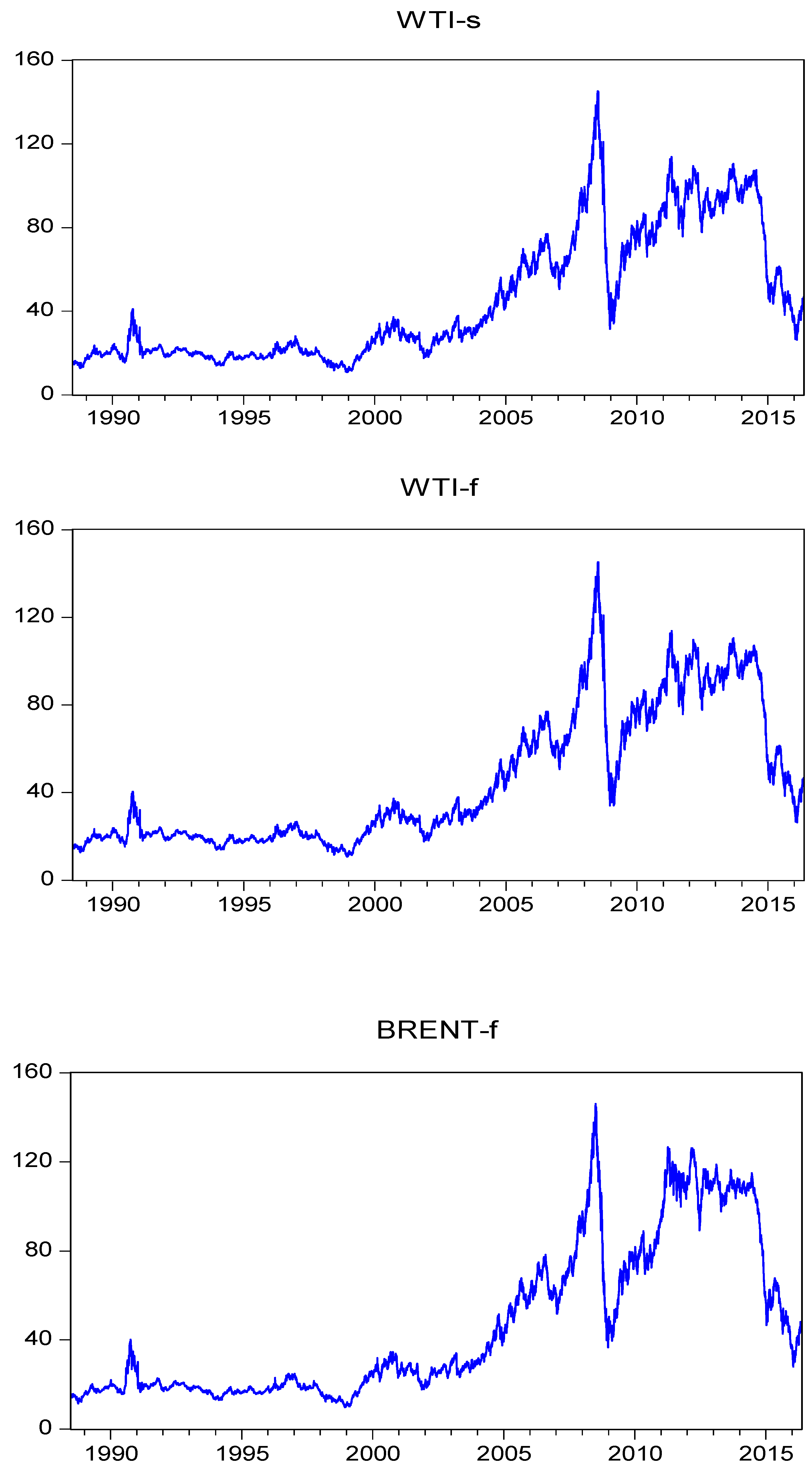
As shown in
Figure 1, which shows the spot and futures price of WTI and futures price of BRENT for 1988–2016, the historical price of spot and futures prices of crude oil in the UK and the USA have had enormous fluctuations since 2007, which coincided with the beginning of the Global Financial Crisis (GFC). Thus, analyzing the correlations and spillovers between crude oil markets and financial markets seems to be very useful for making investment strategies.
A stock index is a weighted average of stock prices of selected listed companies. Weights mostly depend on market capitalization. Stock indexes give investors insights into decision-making by providing a historical perspective of stock market performance. Investors can invest in index mutual funds to expect as good a performance as the market index. Stock index also provides a yardstick for investors to compare with their individual stock portfolios. Stock index can also be used in forecasting movements in the market.
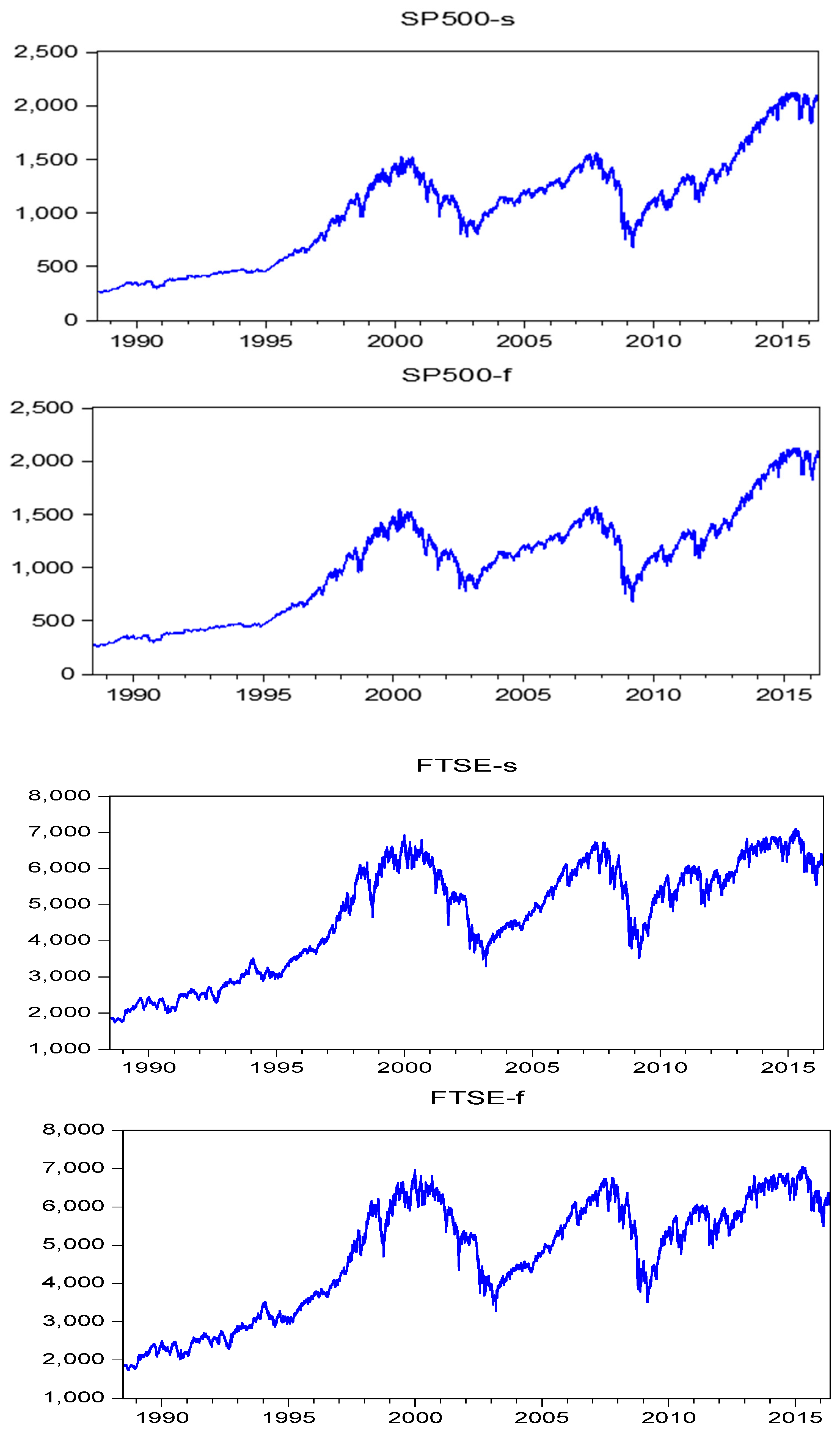
The spot and futures price of S&P 500, and the spot and futures price of FTSE 100 for 1988–2016 are shown in
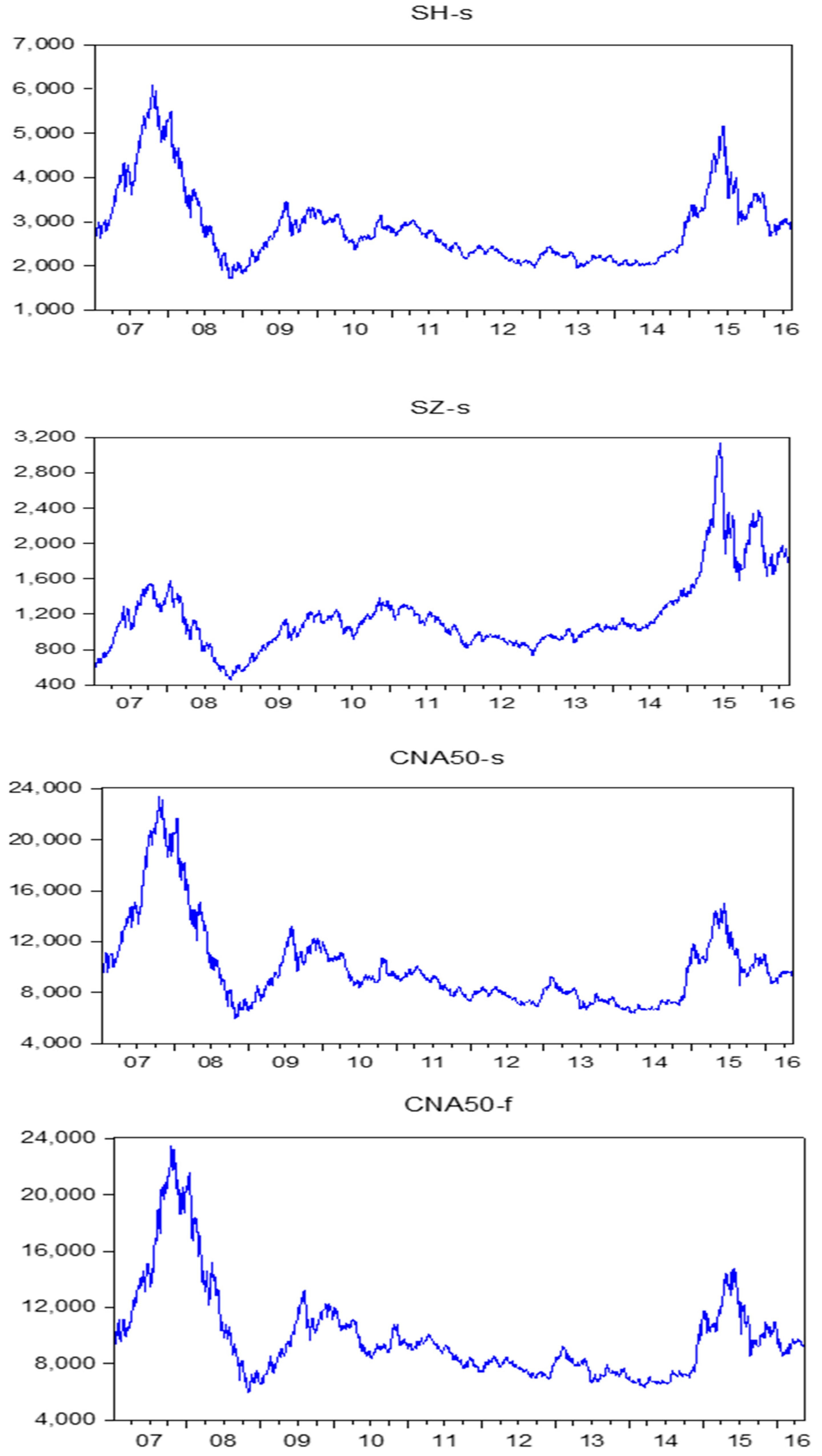
Figure 2, while the spot prices of SSE Composite, SZSE Composite, China A50, and futures price of China A50 for 2007–2016 are shown in
Figure 3. The USA and China are the world’s two largest economies and the UK is the world’s sixth largest economy (and second in the existing EU) behind the USA, China, Japan, Germany, and India. Moreover, the USA and the UK are associated with WTI and Brent oil, respectively.
Given the importance of the Chinese financial and economic systems (see Mao and McAleer (2017) [
1]), it is important to examine how the oil and financial markets vary across the UK, the USA, and China. China hosted a summit on 14–15 May 2017 on its new Silk Road Plan, called the Belt and Road Initiative (BRI) Forum for International Co-operation. In numerous government press releases, it is stated that China intends to build land and sea trade routes linking Asia, Africa, the Middle East, and Europe, based on ancient trade routes. The land route is intended to go through China and Central Asia to Europe, while the sea route is intended to go through South-East Asia to South Asia, Africa, the Middle East, and Europe.
With this in mind, the empirical results for China suggest numerous opportunities for optimal dynamic hedging across the oil and financial markets, as well as with the UK and USA. The empirical results for China also suggest numerous opportunities for optimal dynamic hedging across the oil and financial markets, as well as with the UK and the USA. This is important as the extant literature does not seem to have examined the issue of conditional correlations, conditional covariances, and co-volatility spillovers on optimal hedging strategies.
Volatility is essential in analyzing any markets with high frequency (daily and weekly data) or ultra-high frequency data (second, minute, or hourly data), but it is usually unobservable in commodity and financial markets. Volatility spillovers seem to be widespread in both the crude oil and financial markets. A volatility spillover is the lagged effect on one market due to changes in return shocks in another market. Unfortunately, the analysis of volatility and co-volatility spillovers is typically conducted in a confused and confusing manner, with incorrect definitions and inappropriate models being used, mainly with no standard statistical properties underlying the empirical analysis.
The findings of Arouri et al. (2009) [
2] show significant volatility spillovers between oil price and stock returns. Thus, volatility spillovers and asymmetric effects in crude oil markets and financial markets play important roles in calculating optimal hedge ratios and optimal portfolios.
In an early analysis on the topic of volatility spillovers, Sadorsky (1999) [
3] uses a vector autoregression to show that oil price returns and oil price volatility both play important roles in influencing real stock returns in financial markets. Oil price fluctuations and interest rates were shown to account for approximately 5–6% of the stock return forecast error variance in the USA.
Faff and Brailsford (1999) [
4] find the pervasiveness of an oil price factor, beyond the influence of the market, is detected across some Australian industries. Significant positive oil price sensitivity is found in the oil and gas and diversified resources industries and significant negative oil price sensitivity is found in the paper and packaging and transport industries.
A multivariate vector autoregression was used by Cong et al. (2008) [
5] to investigate the interactive relationships between oil price shocks and the Chinese stock market. The empirical results show that an increase in oil volatility does not affect most stock returns, but may increase the speculative behavior in the mining index and petrochemicals index, which would lead to an increase in their stock returns.
In analyzing six OECD countries, Miller and Ratti (2009) [
6] show that stock market indexes respond negatively to increases in the oil price in the long run. The empirical findings support a conjecture of change in the relationship between real oil prices and real stock prices in the last decade compared with earlier years, which may suggest the presence of several stock market bubbles and/or oil price bubbles since the turn of the Century.
Aloui and Jammazi (2009) [
7] use a two-regime Markov-switching EGARCH model to analyze the relationship between crude oil and stock market returns. Unfortunately, the EGARCH model is well-known not to have any regularity conditions, hence is not invertible and has no asymptotic properties, specifically consistency and asymptotic normality (see McAleer and Hafner (2014) [
8] and Chang and McAleer (2017) [
9]). The paper detects two episodes of Markov-switching time series behavior, specifically, one related to a low mean/high variance regime and the other related to a high mean/low variance regime.
Given the high chance that the expansion is followed by a recession, Jammazi and Aloui (2009) [
10] find that the stock market variables respond negatively and temporarily to crude oil changes during moderate phases in France and expansion phases in the UK and France, but not at levels that would plunge them into a recession phase.
Kilian and Park (2009) [
11] show that the reaction of US real stock returns to an oil price shock differ greatly depending on whether the change in the price of oil is driven by demand or supply shocks in oil markets. Fundamental supply and demand shocks are identified as underlying the innovations to the real price of crude oil. These shocks together explain one-fifth of the long-term variation in US real stock returns.
The effects of oil price shocks on stock returns in a major oil-exporting country, namely Norway, are analyzed in Bjørnland (2009) [
12]. The author shows that increasing of oil prices had a simulating effect on the economy in Norway, which is consistent with the expectation for a country that exports large amounts of crude oil. Specifically, following a 10% increase in oil prices, stock returns increased by 2.5%. The maximum effect is reached after 14–15 months (having increased by 4–5%), after which the effect gradually subsides.
Chang et al. (2013) [
13] investigate the crude oil and financial markets by examining the effect of conditional correlations on volatility spillovers. The alternative models used in the empirical analysis are the CCC model of Bollerslev (1990) [
14], the VARMA-GARCH model of Ling and McAleer (2003) [
15], the VARMA-AGARCH model of McAleer, Hoti, and Chan (2008) [
16], and the DCC model of Engle (2002) [
17].
The paper will apply the diagonal version of the multivariate extension of the univariate GARCH model, namely Diagonal BEKK, as presented in Baba et al. (1985) [
18] and Engle and Kroner (1995) [
19]. Chang et al. (2018) [
20] analyze the literature on volatility and co-volatility spillovers between the energy and agricultural markets, providing and defining useful methodology for testing the effects of such spillovers.
2. Financial Econometrics Methodology
There are alternative multivariate volatility models of conditional covariance for accommodating volatility spillover effects. For example, the Baba, Engle, Kraft, and Kroner (1985) [
18] (BEKK) multivariate GARCH model, the diagonal model of Bollerslev et al. (1988) [
21], the constant conditional correlation (CCC) (specifically, multiple univariate rather than multivariate) GARCH model of Bollerslev (1990) [
14], the vech and diagonal vech models of Engle and Kroner (1995) [
19], the Tse and Tsui (2002) [
22] varying conditional correlation (VCC) model, the Engle (2002) [
17] dynamic conditional correlation (technically, dynamic conditional covariance rather than correlation model; for further details, see McAleer (2018) [
23]) (DCC), the Ling and McAleer (2003) [
15] vector ARMA-GARCH (VARMA-GARCH) model, and the VARMA–asymmetric GARCH (VARMA- AGARCH) model of McAleer et al. (2009) [
16]. For further details on these multivariate static and dynamic conditional covariance models see, for example, McAleer (2005) [
24].
In order to estimate multivariate models, it is necessary to estimate and acquire the standardized shocks from the conditional mean returns shocks. Therefore, the univariate conditional volatility model GARCH and the multivariate conditional covariance models, Diagonal BEKK and the special case of scalar BEKK will be presented briefly.
It is worth emphasizing that the full BEKK model does not have an underlying stochastic process that leads to its derivation. It follows that there are no regularity conditions, including invertibility, and hence no likelihood function. It also follows that there are no derivatives of the likelihood function that will lead to the Hessian matrix and hence no asymptotic properties (for further details, see Chang, Li and McAleer (2018) [
25], Chang and McAleer (2019) [
26], and McAleer (2019a) [
27]).
Consider the conditional mean of returns, which may be univariate or multivariate, as follows:
where the returns,
, represent the log-difference in commodity or financial indexes prices,
,
is the information set available at time
t − 1, and
is an unconditionally homoscedastic, but conditionally heteroskedastic, random error term. In order to derive conditional volatility specifications, it is necessary to specify the stochastic process underlying the returns shocks,
.
Much of the following section follows closely the presentation in McAleer (2005) [
24], McAleer et al. (2008) [
28], Chang, Li and McAleer (2018) [
25], Chang, McAleer and Zuo (2017) [
29], and Chang, McAleer and Wang (2018) [
20].
2.1. Univariate Conditional Volatility Models
Various univariate conditional volatility models are used in single index models to describe individual financial assets and markets. Univariate conditional volatilities can also be used as standardization of the conditional covariances in different multivariate conditional volatility models to estimate conditional correlations, which are especially useful in developing optimal dynamic hedging strategies. The GARCH model, as the most popular univariate conditional volatility model, is discussed below.
Consider the random coefficient autoregressive process of order one:
where
and
is the standardized residual.
Tsay (1987) [
30] derived the ARCH(1) model of Engle (1982) [
31] from Equation (2) as:
where
is conditional volatility, and
is the information set at time
t − 1. The use of an infinite lag length for the random coefficient autoregressive process in Equation (2), with appropriate geometric restrictions (or stability conditions) on the random coefficients, leads to the GARCH model of Bollerslev (1986) [
32]:
where the stability parameter,
, lies in the range (−1, 1). From the specification of Equation (2), it is clear that both
and
should be positive as they are the unconditional variances of two independent stochastic processes.
Asymmetric effects could be added to the GARCH model to derive the GJR model, and the EGARCH specification with asymmetry and leverage could also be considered (for further details, see Caporin and McAleer (2013) [
33], Chang and McAleer (2017) [
9], McAleer (2014) [
34], and McAleer and Hafner (2014) [
8]). However, the primary purpose in presenting univariate models is to discuss the first step in estimating the multivariate models.
The Quasi Maximum Likelihood Estimator (QMLE) of the parameters of ARCH and GARCH have been shown to be consistent and asymptotically normal in several papers. For example, Ling and McAleer (2003) [
15] showed that the QMLE for GARCH(
p,
q) is consistent if the second moment is finite. Moreover, a weak sufficient log-moment condition for the QMLE of GARCH(1,1) to be consistent and asymptotically normal is given by:
which is not easy to check in practice as it involves two unknown parameters and a random variable. The more restrictive second moment condition, namely
, is much easier to check in practice.
In general, the proofs of the asymptotic properties follow from the fact that ARCH and GARCH can be derived from a random coefficient autoregressive process. In this context, McAleer et al. (2008) [
28] provide a general proof of the asymptotic properties of multivariate conditional volatility models that are based on proving that the regularity conditions satisfy the regularity conditions given in Jeantheau (1998) [
35] for consistency and the conditions given in Theorem 4.1.3 in Amemiya (1985) [
36] for asymptotic normality.
2.2. Multivariate Conditional Volatility Models
The multivariate extension of the univariate GARCH model is given in Baba et al. (1985) [
18] and Engle and Kroner (1995) [
19]. In order to establish volatility spillovers in a multivariate framework, it is useful to define the multivariate extension of the relationship between the returns shocks and the standardized residuals, that is,
.
The multivariate extension of Equation (1), namely
, can remain unchanged by assuming that the three components are now
vectors, where
is the number of crude oil or financial assets. The multivariate definition of the relationship between
and
is given as:
where
is a diagonal matrix comprising the univariate conditional volatilities. Define the conditional covariance matrix of
as
. As the
vector,
, is assumed to be
iid for all
elements, the conditional correlation matrix of
, which is equivalent to the conditional correlation matrix of
, is given by
. Therefore, the conditional expectation of (4) is defined as:
Equivalently, the conditional correlation matrix,
, can be defined as:
Equation (5) is useful if a model of is available for purposes of estimating , whereas Equation (6) is useful if a model of is available for purposes of estimating .
Equation (5) is convenient for a discussion of volatility spillover effects, while both Equations (5) and (6) are instructive for a discussion of asymptotic properties, especially for the full BEKK model without appropriate parametric restrictions (for further details, see Chang and McAleer (2019) [
26]). As the elements of
are consistent and asymptotically normal, the consistency of
in (5) depends on consistent estimation of
, whereas the consistency of
in (6) depends on consistent estimation of
.
As both and are products of matrixes and the inverse of the matrix D is not asymptotically normal, even when D is asymptotically normal, neither the QMLE of nor will be asymptotically normal, especially based on the definitions that relate the conditional covariances and conditional correlations given in Equations (5) and (6).
Diagonal BEKK
The vector random coefficient autoregressive process of order one is the multivariate extension of Equation (2), and is given as:
where
and
are
vectors,
is an
matrix of random coefficients, and
Technically, a vectorization of a full (that is, non-diagonal or non-scalar) matrix A to vech A can have dimension as high as , whereas vectorization of a symmetric matrix A to vech A can have dimension as low as . Neither of these possibilities is as small in dimension as m × m, which is required to generate an appropriate BEKK model with any regularity conditions or asymptotic properties.
In a case where
A is either a diagonal matrix, or the special case of a scalar matrix,
, McAleer et al. (2008) [
28] showed that the multivariate extension of GARCH(1,1) from Equation (7), incorporating an infinite geometric lag in terms of the returns shocks, is given as the diagonal (or scalar) BEKK model, namely:
where the matrixes
A and
B must be diagonal (or scalar) for multiplication conformability with the vector,
and matrix,
McAleer et al. (2008) [
28] showed that the QMLE of the parameters of the diagonal, and hence also the scalar, BEKK models are consistent and asymptotically normal, so that standard statistical inference on testing hypotheses is valid. Moreover, as
in Equation (8) can be estimated consistently,
in Equation (6) can also be estimated consistently. However, as explained above, asymptotic normality cannot be proved given the definitions in Equations (5) and (6).
In terms of volatility spillovers, as the off-diagonal terms in the second term on the right-hand side of Equation (8), have typical (i,j) elements , there are no full volatility or full co-volatility spillovers. However, partial co-volatility spillovers are not only possible, but they can also be tested using valid statistical procedures.
2.3. Spillovers
Conditional correlations and spillovers between international crude oil and associate financial markets describe the delayed effect of a returns shock in one commodity or financial asset on the subsequent volatility or co-volatility in another commodity or financial asset.
Define as the conditional covariance matrix of . It follows that:
Full volatility spillovers:
;
Full co-volatility spillovers:
;
Partial co-volatility spillovers:
,
where is returns shocks, and is the conditional covariance matrix of .
Full volatility spillovers occur when the returns shock from financial asset k affects the volatility of a different financial asset i.
Full co-volatility spillovers occur when the returns shock from financial asset k affects the co-volatility between two different financial assets, i and j.
Partial co-volatility spillovers occur when the returns shock from financial asset k affects the co-volatility between two financial assets, i and j, one of which can be asset k.
When m = 2, only full volatility spillovers and partial co-volatility spillovers are possible as full co-volatility spillovers depend on the existence of a third financial asset.
2.4. Dynamic Optimal Hedging Strategies
As investors trade massively in both commodity and financial assets, spillovers can provide investors with a basis to understand and hedge optimally using derivatives in both markets. The optimal dynamic hedge ratio is the size of the futures contract relative to the cash transaction.
According to Chang et al. (2011) [
37], consider the case of an oil company which seeks to protect their exposure in the crude oil spot price by taking a position in a futures financial markets. The return on the oil company’s portfolio of spot and futures position can be denoted as:
where
is the return on holding the portfolio between
t − 1 and
t,
and
are the returns on holding spot and futures positions between
t and
t − 1, and
is the dynamic hedge ratio, that is, the number of futures contracts that the hedger must sell for each unit of a spot commodity on which price risk is borne.
According to Johnson (1960) [
38], the variance of the returns of the hedged portfolio, conditional on the information set available at time
t − 1, is given by
where the terms in the second line of Equation (10), namely
,
, and
, are the conditional variances of the spot and futures returns and the covariance between the spot and futures returns, respectively. The Optimal Hedging Ratios (
OHR) are defined as the value of
which minimizes the conditional variance (risk) of the hedged portfolio returns.
Taking the partial derivative of Equation (10) with respect to
, setting it equal to zero, and solving for
, yields the
conditional on the information available at
t − 1 (see, for example, Baillie and Myers (1991) [
39]):
where returns are defined as the logarithmic differences of spot and futures prices. Estimates of dynamic conditional volatility and co-volatility for purposes of testing spillover effects will be undertaken using alternative univariate and multivariate conditional volatility models, as discussed above.
These issues are important as the extant literature does not seem to have examined the issue of conditional correlations, conditional covariances, and co-volatility spillovers on optimal hedging strategies.
3. Data and Variables
As the topic of the paper is to test co-volatility spillovers in the crude oil and financial markets, important indexes in both markets are taken into consideration and will be discussed below.
3.1. Crude Oil Markets
Two key indexes used in crude oil markets are West Texas Intermediate (WTI) in the USA and Brent Blend Oil Index in the UK. Daily spot and futures price of WTI, and the futures price of Brent, are available from 24 June 1988 to 13 May 2016, but there is no spot price available for Brent. All the crude oil indexes used in the paper are expressed in US dollars and in cents per barrel.
WTI refers to oil extracted from wells in the USA and sent via pipeline to Cushing, Oklahoma. The transportation price of WTI is relatively expensive because supplies are land-locked and cannot be transported in large quantities, as can be done where large container ships are used. WTI oil is very light and sweet, which makes it ideal for the refining of gasoline.
The New York Mercantile Exchange (NYMEX) designates petroleum with less than 0.42% Sulphur as sweet. Higher levels of Sulphur content are called sour crude oil. NYMEX defines light crude oil for domestic USA oil as having an American Petroleum Institute (API) gravity between 37° API (840 kg/m3) and 42° API (816 kg/m3). API gravity is a measure of how heavy or light a petroleum liquid is compared with water. If its API gravity is greater than 10, it is lighter and floats on water; if it is less than 10, it is heavier and sinks. Light crude oil produces a higher percentage of gasoline and diesel, so the price is higher than that of heavy crude oil.
The daily spot price of WTI is available using “Bloomberg West Texas Intermediate (WTI) Cushing Crude Oil Spot Price”. It uses benchmark WTI crude at Cushing, Oklahoma, and other USA crude oil grades trade on a price spread differential to WTI, Cushing. Prices are on a free-on-board basis. WTI crude oil at Cushing, Oklahoma typically trades in pipeline lots of 1000 to 5000 barrels a day, for delivery between the 25th day in one month to the 25th of the following month. These prices are for physical shipments. API gravity is 39°, while the sulfur content is 0.34%. The number of barrels per ton is 7640.
Daily futures price of WTI is available under the designation “CL1 COMDTY” in Bloomberg. It is Generic 1st “CL” Future, which is one-month-front contract, traded at NYMEX. The contract trades in units of 1000 barrels and the delivery point is Cushing, Oklahoma.
Brent Blend refers to oil from four different fields in the North Sea, namely Brent, Forties, Oseberg, and Ekofisk. Crude oil from this region is less “light” and “sweet” than that of WTI, but it is still an excellent product for the refining of diesel fuel, gasoline, and other high-demand products. As the supply is water borne, it is relatively easy to transport large quantities to distant locations.
The daily futures Price of Brent Blend is available under the designation “CO1 COMDTY” in Bloomberg. It is Generic 1st “CO” Future, which is also one-month-front contract, traded at the Intercontinental Exchange (ICE) in the UK. The unit of trading is one or more lots of 1000 net barrels of Brent crude oil.
3.2. Financial Markets
The paper examines three leading financial markets internationally, namely the USA, the UK, and China. Daily data are used for eight indexes, namely S&P 500 Spot, S&P 500 Futures, FTSE 100 Spot, FTSE 100 Futures, SSE Composite Spot, SZSE Composite Spot, China A50 Spot, and China A50 Futures.
For the US market, both daily spot and daily futures prices of the widely-used Standard & Poor’s 500 Composite Index (S&P 500) is accessible from 24 June 1988 to 13 May 2016. S&P 500 is based on the market capitalizations of 500 large companies listed on the NYSE or NASDAQ. It is one of the most suitable representations available of the stock market in the USA, which is expressed in US dollars.
For the UK market, daily spot and daily futures prices of the Financial Times Stock Exchange 100 Index (FTSE 100) are available from 24 June 1988 to 13 May 2016. FTSE 100 is an index of the 100 companies with the largest capitalization listed on the London Stock Exchange. The index is considered a benchmark of prosperity for business under the company law of UK, which is calculated in GDP.
Regarding the Chinese markets, both domestic and non-domestic indexes are considered. In domestic Chinese financial markets, the daily spot price of the Shanghai Stock Exchange Composite Index (SSE Composite) and Shenzhen Stock Exchange Composite Index (SZSE Composite) are seen as the leading indicators of financial market trends in China. The SSE Composite includes all stocks (A shares and B shares) that are traded at the Shanghai Stock Exchange and SZSE Composite calculates all stocks listed on the Shenzhen Stock Exchange.
A shares are denominated in Chinese yuan (CNY) traded by domestic investors, whereas B shares are denominated in foreign currencies traded by qualified international investors. Until 13 May 2016, there were 1140 listed companies are included in SSE Composite and 1808 companies were available in SZSE Composite. Both spot prices are calculated in CNY. SSE Composite is available from 19 December 1990 and SZSE Composite is available from 2 January 1992.
Another important index is the FTSE China A50, which is the benchmark for international investors to access China’s domestic financial market through A Shares. The index incorporates the 50 largest A share companies by market capitalization. Daily spot and futures price of FTSE China A50 are available from 5 January 2007 to 13 May 2016, and are denominated in CNY. As the paper emphasizes hedging strategies in both spot and futures markets, for Chinese financial markets, only data after 5 January 2007 are used when China A50 futures price were initiated.
The paper uses daily time series data from 24 June 1988 to 13 May 2016, where all the data are downloaded from Bloomberg. Three time periods are also analyzed from the whole period due to the Global Financial Crisis (GFC) that occurred between 2007 and 2009, namely pre-GFC (from 24 June 1988 to 4 January 2007), GFC (from 5 January 2007 to 5 March 2009) and post-GFC (from 6 March 2009 to 13 May 2016).
The initial date of the GFC is widely regarded as having started somewhere between November 2007 (the high point of the S&P 500 Composite Index prior to the GFC) to August 2009 (after Lehmann Brothers entered bankruptcy). In the paper, the starting point of the GFC is taken to be the date when the futures price of China A50 became available, namely August 2007. By adding seven months of data, the prices and returns move with slightly lower volatility.
3.3. Descriptive Statistics
The returns of crude oil prices and financial market indexes are calculated on a continuous compound basis, defined as:
where
and
are the closing prices
i of market
j for days
t and
t − 1, respectively. WTI-s, WTI-f, BRENT-f, SP500-s, SP500-f, FTSE-s, FTSE-f, SH-s, SZ-s, CNA50-s, CNa50-f denote returns of WTI spot prices, returns of WTI futures prices, returns of BRENT futures prices, returns of S&P 500 spot prices, returns of S&P futures prices, returns of FTSE 100 spot prices, returns of FTSE 100 futures prices, returns of SSE Composite, returns of SZSE Composite, returns of FTSE China A50 spot prices, and returns of FTSE China A50 futures prices, respectively.
The descriptive statistics for crude oil returns and financial index returns in the UK and the USA for four time periods, which are whole sample (1988–2007), pre-GFC (1988–2007), GFC (2007–2009) and post-GFC (2009–2016), are reported in
Table 1.
All the series present large negative mean returns for the during-GFC period, whereas mean returns for each of the variables are positive for pre-GFC, post-GFC and the whole period. Crude oil returns show a larger standard deviation than financial index returns for all periods, indicating that crude oil markets are more volatile than financial markets, in general, at the aggregate level. Not surprisingly, all the variables have the largest standard deviations for all variables during-GFC.
However, except for futures returns of BRENT, all the maximum values exist during-GFC, indicating that, although crude oil markets and financial markets are volatile during-GFC, large positive returns can be obtained during the same period. As for the minimum value, crude oil returns display large negative returns pre-GFC, due to the fact that, on 16 January 1991, the USA began an air attack against Iraqi military targets, as well as the drawdown of Strategic Petroleum Reserves (SPR) in the USA.
The normal distribution has skewness of zero and kurtosis of 3. Spot and futures returns of WTI show positive skewness during-GFC and post-GFC. Futures returns of BRENT also have positive skewness. These statistics show that post-GFC, crude oil markets have more extreme positive returns. Nevertheless, financial index returns always present negative skewness, except futures returns of S&P 500 during-GFC, indicating that compared with crude oil markets, financial markets are more likely to have extreme negative returns.
All the return series have high kurtosis, suggesting the existence of fat tails. The Jarque-Bera Lagrange Multiplier statistics of all series of returns are statistically significant, indicating non-normality in the distribution of returns.
As shown in
Table 2, descriptive statistics for China during-GFC and post-GFC display similar results to those in
Table 1. SSE Composite, China A50 spot and futures show negative mean returns during-GFC and positive mean returns post-GFC. SZSE Composite has positive mean returns for the during-GFC and post-GFC periods, indicating that, in general, the companies listed on SZSE performed well during-GFC and post-GFC. All returns during-GFC and post-GFC show negative skewness, large kurtosis, and large Jarque-Bera Lagrange Multiplier statistics, indicating that it is likely to have negative returns in Chinese financial markets, on average, and that the returns are not normally distributed.
Table 3 presents the correlation matrix for crude oil and financial markets in the UK and the USA for the pre-GFC, during-GFC, and post-GFC periods. Most of the correlation coefficients between pairs of variables show an increasing trend from pre-GFC to post-GFC, indicating that spot and futures returns for crude oil and financial markets have been more closely tied together in recent years. This empirical regularity strengthens the need and importance of testing for co-volatility spillovers between indexes in crude oil and financial markets.
The highest correlation coefficient in the whole sample is between the spot and futures returns of S&P 500, at 0.974, followed by the spot and futures return correlation coefficient of 0.963. The spot and futures returns are also highly correlated in WTI, at 0.901, and with BRENT, at 0.804. The correlation coefficient between WTI spot returns and BRENT futures returns is 0.795, indicating that returns of oil markets are relatively highly correlated between the UK and the USA.
The financial markets in the UK and the USA are only moderately correlated. The correlation coefficient between spot returns of S&P 500 and FTSE 100 is 0.491. However, by examining the whole sample, returns from crude oil markets and financial markets are slightly correlated. Specifically, the highest correlation coefficient is 0.147 between futures returns of WTI and spot returns of FTSE 100.
Pre-GFC, the correlation coefficients are all negative and close to 0 between the crude oil and financial markets. During-GFC and post-GFC, the two markets become moderately correlated. Specifically, the highest correlation between crude oil and financial markets post-GFC is 0.430, which is between the spot or futures returns of WTI and spot returns of S&P 500.
Table 4 shows the correlations of crude oil in the UK and the USA, and financial markets in China during-GFC and post-GFC. Focusing on the financial markets in China during-GFC and post-GFC, the highest correlation coefficient is 0.948 between SSE Composite returns and China A50 spot returns, followed by 0.930 between spot and futures returns of China A50.
Interestingly, the correlation coefficient between SSE Composite returns and SZSE Composite returns is 0.902, whereas SZSE Composite returns and China A50 spot returns have a correlation coefficient of only 0.783. The reason behind these statistics might be the fact that there are only seven SZSE-listed companies in China A50, so the leading companies in SSE Composite are also included in China A50.
The correlation coefficients between crude oil in the UK and the USA and financial markets in China are generally very low. The highest coefficient is 0.132, which is between futures returns of BRENT and SSE Composite returns post-GFC. Comparing this number with the correlation coefficients between crude oil and financial markets in the UK and the USA, it is only one-third of those in the UK and the USA. These results indicate that China has limited experience regarding trading in international crude oil markets.
In the interests of saving space, the unit root tests of all the variables for all time periods are not reported. In order to summarize the unit root tests results, all prices are found to be nonstationary, while all return series are found to be stationary.
4. Empirical Results
By testing the significance of the estimates of matrix A in the Diagonal BEKK model, the co-volatility spillover effects can be obtained directly. Specifically, if the null hypothesis is rejected, there will exist spillovers from the returns shock of commodity or financial index j at t − 1 to the co-volatility between commodities or financial indexes i and j at t that depend only on the returns shock of commodity or financial index i at t − 1. Estimation of the model in Equations (1) and (2) by QMLE is accomplished by using the EViews 8 econometric software package.
The QMLE of the parameters of the underlying univariate models are not presented as they form the first step in estimating the multivariate Diagonal BEKK model. The estimates of the univariate models typically lead to iid standardized shocks as that is one of the primary purposes in estimating univariate conditional volatility models.
Some diagnostic checks have been used, for example, in Dimitriou et al. (2013) [
40] and Kenourgios et al. (2015) [
41]. The former paper uses the DCC model of Engle (2002) [
17] to examine the global financial crisis and emerging stock market contagion, though they incorrectly cite Tse and Tsui (2002) [
22] as the developers of the model. Tse and Tsui (2002) [
22] actually developed the varying conditional correlation (VCC) model. The latter paper considers intraday exchange rate volatility transmissions across Quantitative Easing (QE) announcements (for further discussion of the difficulty associated with interpreting DCC and VCC as conditional correlation models, see Caporin and McAleer (2013) [
33]).
Both DCC and VCC suffer from fatal flaws in that there are no known underlying stochastic processes that lead to either of the model specifications, no mathematical regularity conditions, including invertibility, which is essential to connect the standardized residuals from the conditional volatility models to the returns shocks, and hence to the observed returns. Consequently, there is no known likelihood function of the parameters given the data and hence no first and second derivatives to generate the Jacobian and Hessian matrixes that are essential for deriving the asymptotic properties of the QMLE. These and related issues are discussed in detail in McAleer (2019b) [
42].
The paper pays particular attention to the different patterns of co-volatility spillovers between two markets across three stages around the GFC. It is worth noting that the extant literature does not seem to have examined this issue. Such comparisons provide greater practical implications and make the findings of the paper more useful to practitioners.
4.1. UK and USA
Table 5,
Table 6,
Table 7,
Table 8,
Table 9 and
Table 10 reports the empirical results of the estimates of matrix
A of the Diagonal BEKK model, with various dimensions for the UK and US markets. The estimates of the coefficients in matrix
A can be interpreted as the weights that each variable have on the co-volatility. Mean return shocks and mean co-volatility spillovers are calculated in order to obtain a more precise interpretation and understanding of the two markets. However, the key estimates for the empirical analysis are the elements of the matrixes
A and
B.
Table 5 shows the estimates of matrix
A using 2 × 2 Diagonal BEKK for spot markets for the UK and the USA for four periods. Specifically, spot returns of WTI are tested with spot returns of S&P 500 and spot returns of FTSE 100, respectively. Thus, for each period, there are two pairs of mean co-volatility spillovers.
From the estimates of matrix
A of the Diagonal BEKK model in
Table 5, all the coefficients are statistically significant at the 1% level. For example, the coefficients are 0.236 and 0.248 for WTI spot and S&P 500 spot prices during the whole sample. The empirical results show that there are spillover effects from the spot returns of WTI at
t − 1 to the co-volatility between WTI spot and S&P 500 spot prices and from the spot returns of S&P 500 at
t − 1 to the co-volatility between WTI spot and S&P 500 spot prices. Similar empirical results and interpretations hold for the pre-GFC, during-GFC, and post-GFC sub-periods.
As highlighted in bold in
Table 5, there are two of eight scalar matrixes
A, which are WTI spot and S&P 500 spot prices for the whole period and WTI spot and FTSE spot prices pre-GFC. The scalar matrix
A shows that the two variables have similar weights on the co-volatility between the pair. If the two variables have different effects on their respective co-volatility, a diagonal matrix
A will be interpreted as appropriate weights. In
Table 5, there are four of eight diagonal matrixes
A, which are highlighted in italics.
The mean return shocks for all pairs of variables are shown alongside the estimates of the weight matrix
A. The highest difference in mean return shocks is between WTI spot and S&P 500 spot prices pre-GFC, at 0.036. The partial co-volatility spillover effects are calculated according to the definition presented in
Section 2. The columns of mean co-volatility spillover effects show that there are significant co-volatility spillovers in all the cases presented.
The largest absolute value of mean co-volatility spillovers in
Table 5 is from spot returns of FTSE 100 to the mean co-volatility between WTI spot and FTSE 100 spot prices during-GFC. It can also be found that the mean co-volatility spillovers have the largest absolute values during-GFC as compared with pre-GFC and post-GFC. These empirical results correspond with the fact that during-GFC, the volatility in crude oil markets and financial markets is higher than in the pre-GFC and post-GFC sub-periods.
Table 5 shows that pre-GFC, the mean co-volatility spillovers have different signs in each of the testing pairs, whereas the mean co-volatility spillovers all have negative signs in the pairs during-GFC and post-GFC. Optimal hedging strategies can be considered if the product of the two mean return shocks is negative. Therefore, there are little or no hedging opportunities between the oil spot and financial spot markets during-GFC and post-GFC, as indicated by the 2 × 2 Diagonal BEKK model, whereas dynamic hedging is possible in the pre-GFC sub-period. These results are important as the
extant literature does not seem to have examined this issue. Table 6 demonstrates the estimates of the weight matrix
A using the 2 × 2 Diagonal BEKK model for futures markets for UK and USA for the four periods. In each period, WTI futures returns are analyzed in combination with S&P 500 returns and FTSE 100 returns. BRENT futures returns are also tested in related to the futures returns of the two financial markets. Therefore, there are four pairs of spillovers tests to be considered for each period.
As shown in
Table 6, all the estimates of the weight matrix
A are significant at the 1% level, indicating that each of the variables has significant impacts on the co-volatility in alternative pairs. Among 16 pairs that are considered, 4 pairs show scalar matrixes
A. WTI futures and FTSE 100 futures, BRENT futures and FTSE 100 futures pre-GFC both demonstrate scalar weights in matrix
A. Of 16 pairs, 7 are found to have diagonal matrixes
A.
The results of the signs for futures mean co-volatility spillovers are similar to those of the spot prices. Positive and negative signs of mean co-volatility spillovers can be seen pre-GFC. The signs are always the same for each pair during-GFC and post-GFC. When the products of the mean return shocks are examined, optimal hedging strategies can only be applied pre-GFC. These results are important as the literature does not seem to have examined this issue for the UK and USA. Moreover, such comparisons provide greater practical implications and make the findings of the paper more useful to practitioners.
A 3 × 3 Diagonal BEKK model can be used if three spot returns, namely WTI spot, S&P 500 spot, and FTSE 100 spot prices, are estimated simultaneously.
Table 7 shows the results of the weight matrix
A in the 3 × 3 Diagonal BEKK model, the mean return shocks, and mean co-volatility spillovers for all sets of three spot prices. All the estimates of matrix
A are statistically significant at the 1% level. For the whole sample period, the coefficients are scalar, whereas the estimates of matrix
A are diagonal in the separate sub-periods pre-GFC, during-GFC, and post-GFC.
The mean co-volatility spillovers have similar results as for the 2 × 2 Diagonal BEKK model. On examination of the whole sample and pre-GFC sub-period, optimal hedging strategies can be considered between WTI spot and S&P 500 spot prices and WTI spot and FTSE 100 spot prices. However, there is little or no opportunity of hedging between these two pairs during-GFC and post-GFC.
Table 8 presents the results of the weight matrix
A in the 4 × 4 Diagonal BEKK model, the mean return shocks, and mean co-volatility spillovers for the UK and US futures markets in the four periods. It is notable that in the post-GFC sub-period, WTI futures, BRENT futures and FTSE 100 futures have similar estimates of the weights, namely 0.217, 0.222, and 0.225, respectively, but S&P 500 futures provide a distinctly different coefficient (at 0.291). As for the results of mean co-volatility spillovers, it confirms the interpretation of the results in
Table 5,
Table 6 and
Table 7. Optimal dynamic hedging is not possible between crude oil futures markets and financial futures markets during-GFC and post-GFC by using a 4 × 4 Diagonal BEKK model.
It would be interesting to analyze the spot and futures markets in pairs.
Table 9 and
Table 10 provide the results of a 7 × 7 Diagonal BEKK model consisting of three crude oil returns, namely WTI spot, WTI futures, and BRENT futures, and four financial index returns, namely S&P 500 spot, S&P 500 futures, FTSE 100 spot, and FTSE 100 futures. As can be seen from the estimates of the weights of matrix
A, all the matrixes are found to be diagonal. Although spot and futures markets are analyzed together to determine mean co-volatility spillovers, similar results are found to hold as in the cases of lower dimensions, namely the crude oil and financial markets in the UK and the USA cannot be hedged using a 7 × 7 Diagonal BEKK model.
These empirical results are important as the literature does not seem to have examined this issue for the UK and the USA. Furthermore, such comparisons provide greater practical implications and make the findings of the paper more useful to practitioners.
4.2. China
Table 11 and
Table 12 present the estimates of the weight matrix
A in the Diagonal BEKK model, mean return shocks, and mean co-volatility spillovers, for the crude oil markets in the UK and USA and the financial markets in China, for the during-GFC and post-GFC sub-periods.
Table 11 shows the results of the 2 × 2 Diagonal BEKK model. All the coefficients of matrix
A are statistically significant at the 1% level. Among the 15 pairs of spillovers that are analyzed, there are nine pairs of variables that display estimates of diagonal matrixes
A. It is worth mentioning that for the post-GFC period, diagonal matrix
A exists in each pair of variables, indicating that post-GFC, Chinese financial markets and crude oil markets in the UK and USA have nearly the same impacts on the co-volatility among any pair of commodities and markets.
These results are important as the literature does not seem to have examined this issue for China. Moreover, such comparisons provide greater practical implications and make the findings of the paper more useful to practitioners.
Interestingly, the results of the mean co-volatility spillovers in Chinese markets are quite different from the empirical results presented for the UK and USA. One of the purposes of the paper was to examine how China might be different from the USA and the UK, which seems to be borne out in the empirical analysis. Positive and negative mean co-volatility spillovers pairs can be seen post-GFC, indicating that there is an opportunity that optimal dynamic hedging strategies can be obtained by using a 2 × 2 Diagonal BEKK model.
Table 12 shows the results of a 5 × 5 Diagonal BEKK model, using three crude oil indexes, namely WTI spot, WTI futures, and BRENT futures, and two financial indexes in China, namely China A50 spot and China A50 futures. The estimates of matrix
A are all statistically significant at the 1% level and all the matrixes are diagonal. In addition, the resulting mean co-volatility spillovers are consistent with the results presented in
Table 9, which demonstrate that it is possible to hedge by using a 5 × 5 Diagonal BEKK model in Chinese financial markets, together with UK and US crude oil markets post-GFC.
As discussed above, these results are important as the literature does not seem to have examined this issue for the UK and the USA. Furthermore, such comparisons provide greater practical implications and make the findings of the paper more useful to practitioners.
5. Concluding Remarks
The main purpose of the paper was to analyze the conditional correlations, conditional covariances, and spillovers between international crude oil and associated financial markets and to analyze data for oil and financial markets for the USA, the UK, and China. The prices of oil and its interactions with financial markets makes it possible to determine the associated prices of financial derivatives, such as carbon emission prices.
The approach taken in the paper is different from others in the literature and the purpose of the paper is to examine the usefulness of modeling and testing volatility spillovers in the oil and financial markets. In view of China’s new Silk Road Plan, called the Belt and Road Initiative (BRI), it is important to examine how the empirical results for China raise numerous opportunities for optimal dynamic hedging across the oil and financial markets, as well as with the UK and the USA.
The oil industry has four major regions, namely the North Sea, USA, Middle East, and South-East Asia. Associated with these four regions are three major financial centers, namely those centered in the UK, the USA, and China, for which the data are more recent. The USA and China are the world’s two largest economies, the UK is the world’s sixth largest economy (and second in the existing EU) behind the USA, China, Japan, Germany, and India. Moreover, the USA and the UK are associated with WTI and Brent oil, respectively.
The paper examined the co-volatility spillover effects between crude oil and financial markets among these three countries by partitioning the whole sample time period from 1988 to 2016 into three representative time periods that are associated with the Global Financial crisis (GFC), namely pre-GFC, GFC, and post-GFC. These results are important as the literature does not seem to have examined this issue for the UK, the USA, and China. One of the purposes of the paper was to examine how China might be different from the USA and the UK, which seems to be borne out in the empirical analysis.
The paper analyzed three crude oil indexes returns and eight financial indexes returns using various dimensions of the multivariate conditional covariance Diagonal BEKK model, from which the conditional covariances were used for testing co-volatility spillovers. Based on these results, dynamic hedging strategies could be suggested to analyze market fluctuations in crude oil prices and associated financial markets.
The empirical findings revealed that, for markets in the UK and the USA, there were significant negative co-volatility spillover effects for any pairs of crude oil and financial indexes during-GFC and post-GFC, whereas for pre-GFC and for the whole sample period, most of the pairs had different signs of co-volatility effects. These empirical results suggested opportunities for optimal dynamic hedging.
However, for China, there were significant negative co-volatility effects for numerous pairs of crude oil indexes and financial indexes during-GFC, but positive and negative signs of co-volatility spillovers in the post-GFC period.
The empirical results for China also suggested numerous opportunities for optimal dynamic hedging across the oil and financial markets, as well as with the UK and the USA. These results are important as the literature does not seem to have examined this issue. Moreover, such comparisons provide greater practical implications and make the findings of the paper more useful to practitioners.


