Modeling Latent Carbon Emission Prices for Japan: Theory and Practice

Abstract

Climate change and global warming are significantly affected by carbon emissions that arise from the burning of fossil fuels, specifically coal, oil, and gas. Accurate prices are essential for the purposes of measuring, capturing, storing, and trading in carbon emissions at regional, national, and international levels, especially as carbon emissions can be taxed appropriately when the price is known and widely accepted. This paper uses a novel Capital (K), Labor (L), Energy (E) and Materials (M) (or KLEM) production function approach to calculate the latent carbon emission prices, where carbon emission is the output and capital (K), labor (L), energy (E) (or electricity), and materials (M) are the inputs for the production process. The variables K, L, and M are essentially fixed on a daily or monthly basis, whereas E can be changed more frequently, such as daily or monthly, so that changes in carbon emissions depend on changes in E. If prices are assumed to depend on the average cost pricing, the prices of carbon emissions and energy may be approximated by an energy production model with a constant factor of proportionality, so that carbon emission prices are a function of energy prices. Using this novel modeling approach, this paper estimates the carbon emission prices for Japan using seasonally adjusted and unadjusted monthly data on the volumes of carbon emissions and energy, as well as energy prices, from December 2008 to April 2018. The econometric models show that, as sources of electricity, the logarithms of coal and oil, though not Liquefied Natural Gas (LNG,) are statistically significant in explaining the logarithm of carbon emissions, with oil being more significant than coal. The models generally displayed a high power in predicting the latent prices of carbon emissions. The usefulness of the empirical findings suggest that the methodology can also be applied for other countries where carbon emission prices are latent.

1. Introduction

Climate change and global warming are two of the most important environmental issues presently facing the international community. Global warming is typically defined as the observed century-scale rise in the average temperature of the Earth’s climate system and its related effects, while climate change refers to change in the statistical distribution of weather patterns, specifically average weather conditions, over an extended period, such as a century. Neither climate change nor global warming refer to changing weather conditions on a daily basis (see [1] Allen and McAleer (2018)).

Both climate change and global warming are significantly affected by carbon emissions that arise from the burning of fossil fuels, specifically coal, oil, and gas. One of the major environmental challenges of the climate policy of the European Union Emissions Trading Scheme (or System) is the reduction and mitigation of greenhouse gas emissions by capturing and storing carbon emissions.

Although the clear leader in the battle to reduce and mitigate the effects of carbon emissions is the European Union, China has also started to mitigate the effects of greenhouse gases through the development of domestic regional carbon emission trading markets, with the goal of extending it to the national level in the near future. The creation of such markets that trade in carbon emissions is intended to establish prices that can be used to buy and sell carbon emissions, and to reduce the harmful effects of such emissions on the social and physical environment.

Accurate prices are essential for the purposes of measuring, capturing, storing, and trading in carbon emissions at the regional, national, and international levels, especially as carbon emissions can be taxed appropriately when the price is known and widely accepted. In the absence of an active trading market for carbon emissions, the prices are typically decided through arbitrary administrative deliberations, and hence are not efficient or even necessarily accurate. In this sense, carbon emission prices are latent.

The purpose of this paper is to price the latent carbon prices through a novel econometric approach that can be used to calculate realized latent prices of carbon emissions as a function of capital (K), labor (L), energy (E) (that is, electricity), and materials (M) inputs. The novelty is in extending the KLEM production function to the multivariate setting, modeling latent carbon emission prices, and providing a novel method of estimating monthly latent carbon emission prices that are based on the observed monthly prices of alternative forms of energy using innovative econometric time series models.

The inputs K, L, and M are typically fixed at a monthly observation interval, and are not readily available on any well-known website, whereas E can be changed daily, so that changes in carbon emissions will depend on changes in E. If prices are assumed to depend on the average cost pricing, the prices of carbon emissions and energy may be approximated by an energy production model with a constant factor of proportionality, so that carbon emission prices are a function of energy prices.

Given the relationship between the prices of carbon emissions and energy, econometric models of the latent carbon emission prices are specified, estimated, evaluated, and used for forecasting carbon emissions prices for Japan, based on monthly data from December 2008 to April 2018. The econometric models will show that, as sources of electricity, the logarithms of coal and oil, though not LNG, as well as a deterministic time trend and a tax change dummy variable, are statistically significant in explaining the logarithm of carbon emissions, with oil being more significant than coal.

The plan of the remainder of the paper is as follows. A review of the literature on pricing carbon emissions for the European Union, and at the regional and national levels for China, is given in Section 2. Section 3 discusses the KLEM production function that obtains prices for the output of carbon emissions as a function of the inputs of capital, labor, energy (or electricity), and materials. The formal models of latent carbon emission prices are discussed in Section 4, estimation of the models is presented in Section 5, the monthly data and diagnostic checks are analyzed in Section 6, the empirical estimates and analysis are evaluated in Section 7, and some concluding remarks are given in Section 8.

Proof of the derivation of the correct standard errors for valid statistical inference for realized latent carbon emissions and the ranking of important underlying factors, a discussion on the theoretical structure for latent endogenous and exogenous variables, and extensions to more complicated decision strategies, are given in the Appendix A.

2. Literature Review

Much of the research literature on pricing carbon emissions in recent years has concentrated on Europe and China. The European Union Emissions Trading Scheme established the world’s first greenhouse gas emissions trading scheme in 2005, and remains the largest and most influential organization mitigating the effects of global warming and climate change.

In the sparse literature for Europe, most of which has been based on the European Union Emissions Trading Scheme (EUETS), [2] Daskalakis and Mrkellos (2009) developed a framework for future pricing and hedging, and examined data from EEX, Nord Pool, and Powernext, to analyze whether electricity risk premia were affected by the prices of emission allowances. [3] Daskalakis et al. (2009) provided evidence from modeling the prices of CO₂ emissions allowances and derivatives using European Trading Scheme data.

More recently, [4] Bushnell et al. (2013) examined profiting from regulation, based on European carbon market data. [5] Oestreich and Tsiakas (2015) analyzed carbon emissions and stock returns using EUETS data. Additionally, [6] Martin et al. (2016) examined the impacts of the EUETS on regulated firms for ten years from inception.

China’s market for national carbon emissions was established at a later stage than in Europe, and has been progressing steadily. The development of such markets since their inception in China in 2013 has not necessarily been based on competitive market principles. The National Government in Beijing has made it clear that the regional markets are a first step in the development of a national carbon emission pricing scheme. Just as the market for carbon emissions trading is presently at a formative stage in China, the academic theoretical and empirical research on the emerging regional and national carbon emissions pricing markets is also at a development stage.

A review of the admittedly sparse literature on the prices of carbon emissions in Europe and China, as well as a comprehensive analysis regarding the availability of price data at the domestic regional level, is analyzed in [7,8] Chang et al. (2018, 2019). Following earlier work, the authors discuss a number of developments in China since 2005. [9] Chen (2005) evaluated the costs associated with mitigating carbon emissions. [10] Gregg et al. (2008) analyzed the carbon emissions patterns associated with fossil fuel consumption and cement production. Moreover, [11] Li and Colombier (2009) evaluated carbon emissions and energy efficiency. Using a multivariate modeling approach, [12] Chang (2010) developed a multivariate causality test of various combinations of carbon dioxide emissions, energy consumption, and economic growth.

In more recent years, there have been analyses of interactions between China and one or more other regions. For example, [13] Nam et al. (2014) compared the synergy between China and the USA associated with pollution and carbon emissions controls. For China alone, [14] Zhang et al. (2014) considered the effects of emissions trading on progress and future prospects, [15] Zhang et al. (2014) used the Shapley value to analyze carbon emissions quotas across regions, [16] Liu et al. (2015) reviewed trading in carbon emissions and future challenges, [17] Tang et al. (2015) evaluated the trading scheme for carbon emissions using a multi-agent-based model, and [18] Zhang (2015) reformulated a strategy for low-carbon green growth. [19] Xiong et al. (2017) provided a comparison of China’s carbon trading allowance scheme and related schemes in the EU and California.

There seems to be even less research on pricing carbon emissions at an international level. [20] Zhang and Sun (2016) applied a Full BEKK multivariate conditional volatility model to analyze the time-varying covariances and the associated dynamic spillovers between the respective markets for Euro carbon and fossil fuel (for caveats regarding the Full BEKK model, particularly regarding the lack of mathematical regularity conditions, invertibility, the absence of a likelihood function, and hence the lack of valid asymptotic statistical properties, see [21] Chang and McAleer (2019)) [22]. Chang et al. (2017) and [21] Chang and McAleer (2019) analyzed the novel issues of volatility spillovers and Granger causality on the basis of daily data for the futures prices of EU carbon emissions, spot prices of US carbon emissions, and spot and future prices of oil and coal.

Interesting recent research has been undertaken on analyses of price and volatility from the perspective of derivative markets and alternative volatility models, such as the price impact, trading volume and volatilities associated with mission permits and the announcement of realized emissions in [23] Hitzemann, Uhrig-Homburg, and Ehrhart (2015); a Bayesian approach to the stochastic volatility of future prices of emission allowances in [24] Kim, Park, and Ryu (2017); and the empirical performance of reduced form models for emission permit prices in [25] Hitzemann and Uhrig-Homburg (2019).

As stated above, there seems to have been no published research on pricing carbon emissions in Japan. The existing published research seems to have primarily focused on Europe and, very recently, China. For these reasons, this paper makes a novel contribution to the pricing of carbon emissions for Japan. The usefulness of the empirical findings suggests that the methodology can also be applied for other countries where carbon emission prices are latent.

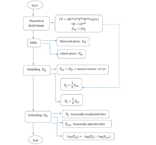
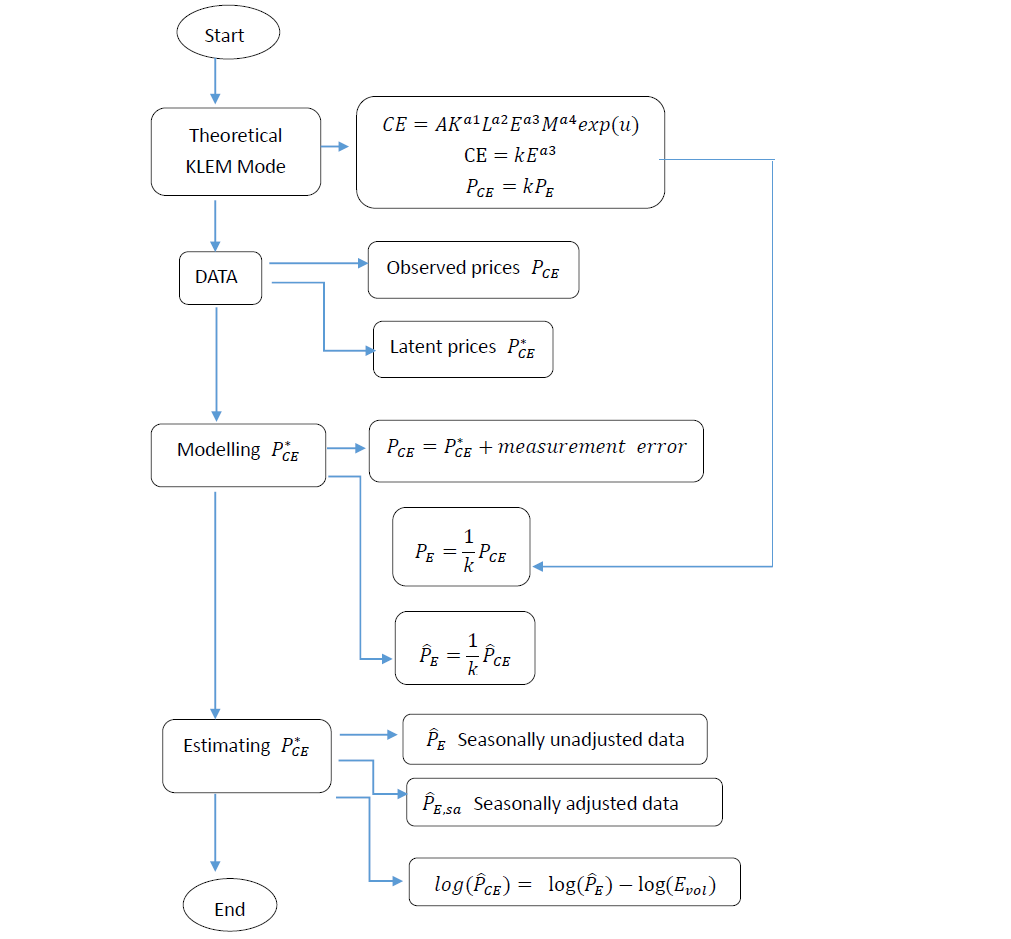
3. KLEMS Production Function for Carbon Emissions and Energy

Inputs are required to produce outputs, and the relationship is captured in a production function. A relatively broad specification is the KLEMS production function ([26] OECD, 2001), which uses capital ($K$), labor ($L$), energy ($E$), materials ($M$), and services (S) as the inputs for the production process. The function captures the most widely-used inputs for producing the output. Typically, the most widely observable input is energy, which is based on the use of electricity, whereas the services associated with a specific output are typically difficult to observe.

As a special case of KLEMS, consider the KLEM production function (see, for example, [27] Lecca et al., 2011) that is given as

$$CE=A{K}^{a1}{L}^{a2}{E}^{a3}{M}^{a4}exp\left(u\right),$$

(1)

where CE denotes the production of the output of carbon emissions; capital ($K$), labor ($L$), energy or electricity ($E$), and materials ($M$) are the inputs; $A$ is a constant; for simplicity, the partial production parameters are assumed to satisfy constant returns to scale, that is, $a1+a2+a3+a4=1$ (as in the Cobb-Douglas production function); and the random error term is assumed to be $u~iid\left(0,1\right).$

In practice, the output $CE$ and input $E$ may be observed at daily or monthly data frequencies, whereas the inputs $K$, $L$, and $M$ are generally fixed at much lower data frequencies, such as one year. Consequently, when the data are observed at monthly frequencies, as in this paper, $CE$ and $E$ may be assumed to be proportional, with the random factor of proportionality given by

$$k=A{K}^{a1}{L}^{a2}{M}^{a4}exp\left(u\right).$$

(2)

It is worth noting that $k$ is not restricted in its range, such as (0, 1). As $k$ has a unit of measurement, $k$ can take any value, depending on the units of measure of the variables, such as

$$CE=k{E}^{a3}$$

(3a)

or

$$\log \left(CE\right)=\log \left(k\right)+a3\log \left(E\right),$$

(3b)

where $a3$ is a scalar. If it is assumed that output prices are set according to an average cost pricing rule (see [28] Chang et al. (2018)), the prices of $CE$ and $E$ may be approximated by a model with a constant factor of proportionality. Let this relationship be given as

$$P_{CE}=k{P}_E,$$

(4)

where $P_{CE}$ is the price of $CE$, and $P_E$ is the price of energy (such as electricity), such that k in Equation (4) is the constant factor of proportionality. In practice, k may be known in advance or may be determined empirically using appropriate modeling techniques. [28] Chang et al. (2018) considered estimating k through the use of Equations (3b) and (4). The estimation of $P_{CE}$ through the use of econometric models, and acknowledging the presence of measurement errors, will be developed in the next section.

4. Modeling Latent Carbon Emission Prices

The definitional relationship for a random variable, Y, can be seen in Equation (5):

Y = Y* + measurement error,

(5)

where Y is the measured value of the random variable, which is subject to measurement error, and Y* is the true value of the random variable, with no measurement error, for which the following four relationships are possible:

(i)

$Y=P_{CE}, Y^{*}=P_{CE}^{*}$;

(ii)

$Y=P_{CE}, Y^{*}=P_E^{*}$;

(iii)

$Y=P_E, Y^{*}=P_E^{*}$;

(iv)

$Y=P_E, Y^{*}=P_{CE}^{*}$.

Here, $P_{CE}$ and $P_{CE}^{*}$ denote the (possibly) observed prices of carbon emissions and their underlying true prices, respectively, and $P_E$ and $P_E^{*}$ denote the observed and underlying true prices of energy, respectively.

In cases (i) and (ii), the price of carbon emissions is not available, together with the true underlying prices of carbon emissions and energy, respectively. case (iii) is not of particular interest as it relates to the observed and true underlying prices of energy, respectively. In case (iv), the price of energy is available, but the true underlying price of carbon emissions is not. Therefore, this paper is concerned with case (iv).

The remainder of the paper uses a novel econometric model to calculate the latent prices of carbon emissions, as will be discussed below. The approach has been used in the literature to calculate latent variables, and this paper is the first to use the methodological approach to calculate latent carbon emission prices.

For the sake of argument, in case (iv), if the price of energy is stationary, $P_E$ can be regressed on a set of observable variables using Ordinary Least Squares (OLS), as given in Equation (6):

$$P_E=b_0+b_1{Z}_1+b_2{Z}_2+b_3{Z}_3+error,$$

(6)

to yield estimated fitted values, as given in Equation (7):

$$\widehat{P_E}=\widehat{b_0}+\widehat{b_1}{Z}_1+\widehat{b_2}{Z}_2+\widehat{b_3}{Z}_3=\frac{1}{k}\widehat{P_{CE}^{*}},$$

(7)

where $\widehat{b_i}$ denotes the OLS estimates of the unknown parameters $b_i$ (i = 0, 1, 2, 3), and $\widehat{P_E}$ denotes the estimated fitted values of energy prices from Equation (6), which are equivalent to the estimated fitted values of carbon emissions, ($\widehat{P_{CE}^{*}}$), adjusted by the factor (1/k) (see Equation (4)), where k may be known in advance or may be determined empirically.

If energy prices are nonstationary rather than stationary, the price model for energy in Equation (6) can be estimated using a cointegrating relationship or a vector autoregressive distributed lag model to accommodate the nonstationarity. Alternatively, prices can be transformed into log differences in prices, which are equivalent to the rate of growth in prices, and then estimated by OLS (in empirical finance, log differences in prices are referred to as rates of return), which would be based on stationary processes.

5. Estimating Latent Carbon Emission Prices

This section describes a novel method of estimating monthly latent carbon emissions prices for Japan that are based on the observed monthly prices of alternative forms of energy and the models presented in the previous section.

Monthly prices (p) and volumes (quantities, q) of the following energy variables are typically available in a variety of energy databases, where almost ethanol refers to bio-ethanol:

(1)

Volume of carbon emissions;

(2)

Prices and volume of electricity;

(3)

Prices and volume of oil;

(4)

Prices and volume of crude coal;

(5)

Prices and volume of natural gas;

(6)

Prices and volume of nuclear energy;

(7)

Prices and volume of solar energy;

(8)

Prices and volume of wind energy;

(9)

Prices and volume of hydro energy;

(10)

Prices and volume of wave energy;

(11)

Prices and volume of bio-mass;

(12)

Prices and volume of ethanol;

(13)

Prices and volume of bio-ethanol.

In what follows, the models presented in the previous section will be estimated using the available price and volume data to obtain estimated fitted latent prices of carbon emissions. It is assumed that there is a known expected relationship between carbon emissions and the generation of electricity using the data in cases (2)–(12) above. This is based on applied engineering practice and structural form modeling, as presented in the previous section, as follows:

$$p_0{q}_0=k{p}_1{q}_1\exp \left(u\right)$$

(8)

or equivalently as

$$\log (p_0{q}_0)=\log \left(k\right)+\log \left(p_1{q}_1\right)+u,$$

(9)

where k is assumed to be a known factor of proportionality, and u is assumed to be a random measurement error, possibly independently and identically distributed, with a mean of 0 and constant variance.

Equation (8) relates the unknown price and known quantity of carbon emissions to the known price and known quantity of energy (or electricity), which confirms that the resulting price equation directly refers to carbon emissions. Equation (9) is the logarithmic equivalent of Equation (8).

Let $pq=e$ (expenditure), with $k=1$, without a loss of generality, so that Equation (8) becomes

$$\log \left(e_0\right)=\log \left(e_1\right)+u.$$

(10)

It follows that

$$\mathrm{E}\left[\log \left(e_0\right)\left]=E\right[\log \left(e_1\right)\right]$$

(11)

as $\mathrm{E}\left(u\right)=0$, such that the estimated fitted value of Equation (10) is given as

$$\widehat{\log \left(e_0\right)}=\widehat{\log \left(e_1\right)}.$$

(12)

A regression of $\log \left(e_1\right)$ on $\log \left(e_2\right),\dots ,\log \left(e_{12}\right)$ gives

$$\log \left(e_1\right)=c+{\delta }_2\log \left(e_2\right)+\dots +{\delta }_{12}\log \left(e_{12}\right)+error,$$

(13)

for which the estimated fitted value of $log\left(e_1\right)$ is given as

$$\widehat{\log \left(e_1\right)}=\widehat{c}+\widehat{{\delta }_2}\log \left(e_2\right)+\dots +\widehat{{\delta }_{12}}\log (e_{12}),$$

(14)

where $\widehat{c}, \widehat{{\delta }_2 },\dots ,\widehat{{\delta }_{12}}$ are the OLS estimates of $c, {\delta }_2,\dots ,{\delta }_{12}$, respectively.

Recalling Equation (11), it follows that

$$\widehat{\log \left(e_0\right)}=\widehat{\log \left(e_1\right)}= \widehat{c}+\widehat{{\delta }_2}\log \left(e_2\right)+\dots +\widehat{{\delta }_{12}}\log \left(e_{12}\right),$$

(15)

which gives an “optimal” estimate of $\log \left(e_0\right)$.

As $\log \left(e_0\right)=\log \left(p_0{q}_0\right)$ and $\widehat{\log e_0}=\widehat{\log \left(p_0\right)}+\log q_0$, the prices of carbon emissions can be “optimally” calculated as

$$\widehat{\log \left(p_0\right)}=\widehat{\log \left(e_0\right)}-\log \left(q_0\right).$$

(16)

Equation (16) gives the estimated fitted value, $\widehat{\log p_0}$, as the “optimal” estimate of carbon emission prices as it uses valid statistical techniques that are efficient and optimal.

This novel method would seem to be the first to calculate carbon emissions prices in theory, as well as in practice, using monthly data for Japan.

Further to the above discussion, if data were available for $p_0$, the price of energy (or electricity), as well as prices on some renewable ($Z_1$, say) and nonrenewable ($Z_2$, say) energy inputs, we could compare whether $Z_1$ jointly was more or less significant than $Z_2$ in explaining $p_0$.

The Japanese Government imposes energy taxes on industry, in particular, as well as on households. The use of government data is crucial for consumers and businesses that use energy, as they are expected to pay carbon taxes as users of energy. This is not a financial product, but an application of optimal carbon tax policies.

6. Monthly Data and Diagnostic Checks

The empirical analysis uses a monthly sample period from December 2008 to April 2018 for Japan, where carbon emission prices have not yet been calculated by any government agency or research institute. The definitions of the variables are given in

Table 1. Definition of variables.

Variable	Definition	Source
$Coal$	Value of coal (Import value of coal)	Trade Statistics of Japan, Ministry of Finance
$Coa{l}_{SA}$	Value of coal seasonally adjusted by X12
$LNG$	Value of LNG (Import value of LNG)	Trade Statistics of Japan, Ministry of Finance
$LN{G}_{SA}$	Seasonally adjusted value of LNG
$Oil$	Value of petroleum (Import value of petroleum)	Trade Statistics of Japan, Ministry of Finance
$Oi{l}_{SA}$	Value of petroleum seasonally adjusted by X12
$E$	Value of electricity obtained by P_E × E vol
$E_{SA}$	Value of electricity seasonally adjusted by X12
$CE$	Volume of carbon emission (ppm) Average of observations	Japan Metrological Agency
$C{E}_{SA}$	Volume of carbon seasonally adjusted by X12
$P_E$	Spot electricity price (Day ahead, 24 h)	Japan Electricity Power eXchange
$E_{vol}$	Total transaction volume of electricity	Japan Electricity Power eXchange
$E_{vol,SA}$	Total transaction volume of electricity seasonally adjusted by X12

Note: The sample period is monthly from December 2008 to April 2018.

as the volume of seasonally unadjusted and seasonally adjusted (using X12) values of coal, LNG, petroleum, electricity, carbon emissions, the spot electricity price, the total transaction volume of electricity, and the price of electricity that represents the price of energy. The sources of the data are the Trade Statistics of Japan, Ministry of Finance, Government of Japan; the Japan Metrological Agency; and the Japan Electricity Power eXchange.

Prior to econometric estimation, the seasonally unadjusted and adjusted volumes of the logarithms of electricity, coal, oil, and LNG were tested for unit roots, for both levels and first differences of the variables, using the non-parametric Phillips-Perron (PP) test of stationarity to ensure that asymptotic theory was valid for the purposes of drawing statistical inferences (see [29] Phillips and Perron (1979)). The test of the null hypothesis that a time series is integrated by an order of 1 is robust to unspecified autocorrelation and heteroscedasticity in the errors of the auxiliary test equation.

The PP tests of the logarithms of the levels and first differences of the seasonally unadjusted and adjusted volumes of electricity, coal, oil, and LNG in

Table 2. Phillips-Perron unit root tests.

(a) Levels
Variable	Test Statistic	p-value
$\log \left(E\right)$	−2.320	0.420
$\log \left(E\right)\log {\left(E\right)}_{SA}$	−1.209	0.904
$\log \left(Coal\right)$	−3.309	0.070
$\log {\left(Coal\right)}_{SA}$	−2.727	0.228
$\log \left(Oil\right)$	−2.541	0.308
$\log {\left(Oil\right)}_{SA}$	−2.069	0.557
$\log \left(LNG\right)$	−2.166	0.504
$\log {\left(LNG\right)}_{SA}$	−1.321	0.878
Notes: SA denotes a seasonally adjusted variable. The auxiliary regression included a constant term and time trend. OLS was used to obtain the estimator of the residual spectrum at a frequency of zero.
(b) First Differences
Variable	Test Statistic	p-value
$\Delta \log \left(E\right)$	−11.862	0.000
$\Delta \log {\left(E\right)}_{SA}$	−10.960	0.000
$\Delta \log \left(Coal\right)$	−15.262	0.000
$\Delta \log {\left(Coal\right)}_{SA}$	−14.411	0.000
$\Delta \log \left(Oil\right)$	−12.241	0.000
$\Delta \log {\left(Oil\right)}_{SA}$	−12.639	0.000
$\Delta \log \left(LNG\right)$	−32.051	0.000
$\Delta \log {\left(LNG\right)}_{SA}$	−11.336	0.000
Notes: SA denotes a seasonally adjusted variable. The auxiliary regression included a constant term. The number of lags for the auxiliary regression was determined by the Akaike Information Criterion (AIC). Ordinary Least Squares (OLS) was used to obtain the estimator of the residual spectrum at a frequency of zero.

were conducted using a constant term with a deterministic trend in order to provide alternative simulated critical values of the non-standard test. OLS was used to obtain the estimator of the residual spectrum at a frequency of zero. The PP test detects unit roots of the logarithmic levels of the variables at all reasonable levels of significance, but rejects the null hypothesis of unit roots in logarithmic first differences, so that the log differences of the data are stationary.

The correlations in the logarithmic levels of the seasonally unadjusted and adjusted data are shown in

Table 3. (a) Correlation: Levels. (b) Correlation: First differences.

(a) Seasonally unadjusted data
	$\mathbf{log}\left(\mathit{E}\right)$	$\mathbf{log}\left(\mathit{Coal}\right)$	$\mathbf{log}\left(\mathit{Oil}\right)$	$\mathbf{log}\left(\mathit{LNG}\right)$
$\log \left(E\right)$	1.000	0.159	−0.008	0.379
$\log \left(\mathit{Coal}\right)$	0.159	1.000	0.317	0.341
$\log \left(\mathit{Oil}\right)$	−0.008	0.317	1.000	0.730
$\log \left(\mathit{LNG}\right)$	0.379	0.341	0.730	1.000
Seasonally adjusted data
	$\mathbf{log}{\left(\mathit{E}\right)}_{\mathit{S}\mathit{A}}$	$\mathbf{log}{\left(\mathit{Coal}\right)}_{\mathit{S}\mathit{A}}$	$\mathbf{log}{\left(\mathit{Oil}\right)}_{\mathit{S}\mathit{A}}$	$\mathbf{log}{\left(\mathit{LNG}\right)}_{\mathit{S}\mathit{A}}$
$\log {\left(E\right)}_{SA}$	1.000	0.146	−0.008	0.375
$\log {\left(\mathit{Coal}\right)}_{SA}$	0.146	1.000	0.294	0.295
$\log {\left(\mathit{Oil}\right)}_{SA}$	−0.008	0.294	1.000	0.737
$\log {\left(\mathit{LNG}\right)}_{SA}$	0.375	0.295	0.737	1.000
(b) Seasonally unadjusted data
	$\mathbf{\Delta }\mathbf{log}\left(\mathit{E}\right)$	$\mathbf{\Delta }\mathbf{log}\left(\mathit{Coal}\right)$	$\mathbf{\Delta }\mathbf{log}\left(\mathit{Oil}\right)$	$\mathbf{\Delta }\mathbf{log}\left(\mathit{LNG}\right)$
$\Delta \log \left(E\right)$	1.000	0.066	0.125	0.211
$\Delta \log \left(\mathit{Coal}\right)$	0.066	1.000	0.299	0.401
$\Delta \log \left(\mathit{Oil}\right)$	0.125	0.299	1.000	0.445
$\Delta \log \left(\mathit{LNG}\right)$	0.211	0.401	0.445	1.000
Seasonally adjusted data
	$\mathbf{\Delta }\mathbf{log}{\left(\mathit{E}\right)}_{\mathit{S}\mathit{A}}$	$\mathbf{\Delta }\mathbf{log}{\left(\mathit{Coal}\right)}_{\mathit{S}\mathit{A}}$	$\mathbf{\Delta }\mathbf{log}{\left(\mathit{Oil}\right)}_{\mathit{S}\mathit{A}}$	$\mathbf{\Delta }\mathbf{log}{\left(\mathit{LNG}\right)}_{\mathit{S}\mathit{A}}$
$\Delta \log {\left(\mathit{E}\right)}_{SA}$	1.000	0.043	0.177	0.038
$\Delta \log {\left(\mathit{Coal}\right)}_{SA}$	0.043	1.000	0.267	0.267
$\Delta \log {\left(\mathit{Oil}\right)}_{SA}$	0.177	0.267	1.000	0.200
$\Delta \log {\left(\mathit{LNG}\right)}_{SA}$	0.038	0.267	0.200	1.000

(a), with the corresponding correlations in the logarithmic first differences of the seasonally unadjusted and adjusted data shown in Table 3(b). The highest correlations for the logarithmic levels of the seasonally unadjusted and adjusted data are between oil and LNG, with surprisingly close values of 0.73 and 0.737, respectively. The highest correlations for the logarithmic first differences of the seasonally unadjusted and adjusted data are quite different, with the highest correlation for the former being between oil and LNG at 0.445, and at a much lower 0.267 for coal and oil, as well as for coal and LNG.

The [30] Johansen (1991) Trace and Maximum Eigenvalue tests of the number of cointegrating vectors for the seasonally unadjusted and adjusted values of coal, LNG, oil, and electricity are presented in

Table 4. Johansen Trace and Maximum Eigenvalue tests of cointegrating vectors.

Trace or Maximum Eigenvalue Test	Number of Cointegrating Vectors	Test Statistic (p-Value)
Trace $\log \left(Coal\right),\log \left(LNG\right),\log \left(Oil\right),\mathrm{and}\log \left(E\right)$	$R=0$	66.725 (0.028)
Maximum Eigenvalue $\log \left(Coal\right),\log \left(LNG\right),\log \left(Oil\right),\mathrm{and}\log \left(E\right)$	$R=0$	37.215 (0.011)
Trace $\log {\left(Coal\right)}_{SA},\log {\left(LNG\right)}_{SA},\log {\left(Oil\right)}_{SA},\mathrm{and}\log {\left(E\right)}_{\mathrm{SA}}$	$R=0$	77.143 (0.003)
Maximum Eigenvalue $\log {\left(Coal\right)}_{SA},\log {\left(LNG\right)}_{SA},\log {\left(Oil\right)}_{SA},\mathrm{and}\log {\left(E\right)}_{\mathrm{SA}}$	$R=0$	40.017 (0.004)

Notes: SA denotes a seasonally adjusted variable. R is the number of cointegrating vectors.

. The null hypothesis of no cointegration (that is, R = 0) can be rejected at the 5% level of significance using both tests for the combination of logarithms of the seasonally unadjusted and adjusted volumes of coal, LNG, oil, and electricity.

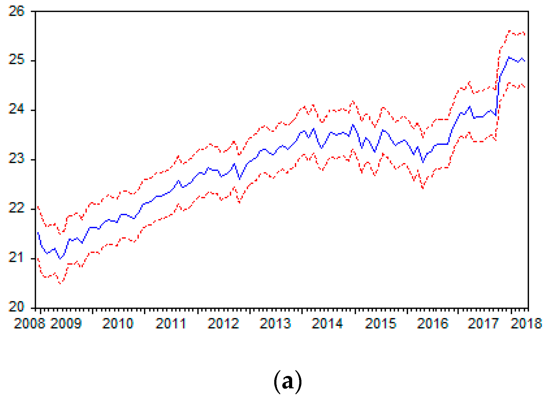
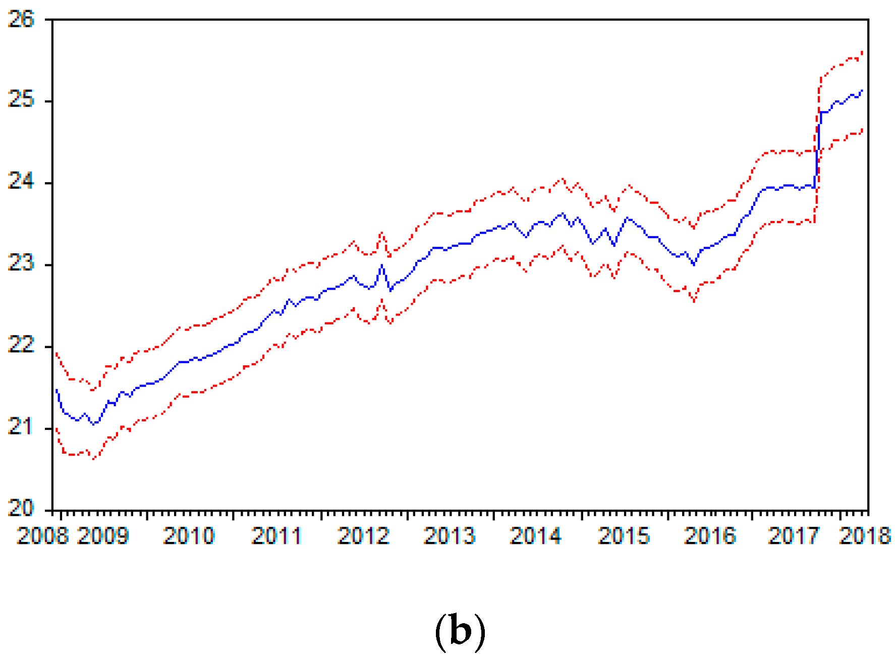
7. Empirical Estimates and Analysis

The results of the PP unit root tests and Johansen tests of the number of cointegrating vectors in the previous section led to fully-modified OLS estimation ([31] Phillips and Hansen, 1990) of the cointegrating regressions, presented in

Table 5. Cointegrating regression (fully-modified OLS) for carbon emissions. Case 1: Seasonally unadjusted data. Case 2: Seasonally adjusted data.

	Case 1	Case 2
Constant	−3.180 (0.409)	−4.141 (0.253)
$\log (Coal)$	0.410 (0.056) *
$\log {\left(Coal\right)}_{SA}$		0.451 (0.025) **
$\log (LNG)$	0.215 (0.210)
$\log {\left(LNG\right)}_{SA}$		0.265 (0.125)
$\log (Oil)$	0.612 (0.001) ***
$\log {\left(Oil\right)}_{SA}$		0.573 (0.002) ***
Trend	0.027 (0.000) ***	0.026 (0.000) ***
Dummy	0.669 (0.000) ***	0.772 (0.000) ***
Adjusted R2	0.943	0.958

Notes: ***, **, and * denote statistical significance at the 1%, 5%, and 10% levels, respectively. Numbers in parentheses indicate p-values of the t-tests. The dummy variable, which was introduced to accommodate the influence of increases in electricity prices on May 2017 arising from tax changes in Japan, equals 0 before September 2017, and 1 after September 2017.

.

Two cases are considered, as follows:

• Case 1: Seasonally unadjusted data, with a deterministic trend and dummy variable;
• Case 2: Seasonally adjusted data, with a deterministic trend and dummy variable.

The dummy variable, which was introduced to accommodate the influence of increases in electricity prices on May 2017 arising from tax changes in Japan, equals 0 before September 2017, and 1 after September 2017.

For both seasonally unadjusted and seasonally adjusted data, that is, Cases 1 and 2, the logarithms of coal and oil, as well as the deterministic time trend and the tax change dummy variable, are statistically significant in explaining the logarithm of carbon emissions, with oil being more significant than coal. The logarithm of LNG is not statistically significant at any conventional level of significance in explaining the logarithm of carbon emissions in either Case 1 or Case 2. The adjusted R² values are reasonably high, at 0.943 and 0.958 for Cases 1 and 2, respectively, which suggests that the models are quite successful in explaining the logarithm of carbon emissions using both seasonally unadjusted and seasonally adjusted data.

The forecasts of $\log \left(E\right)$ for seasonally unadjusted and seasonally adjusted data are shown in Figure 1a,b, respectively, where two standard errors in each figure provide the 95% confidence intervals. In each case, there were noticeable falls in the forecasts of the logarithm of electricity from mid-2015 through to early-2016, and substantial rises toward the end of 2017.

The predicted latent carbon emission prices for seasonally unadjusted and adjusted data are depicted in Figure 2a,b respectively.

The predicted values are based on the formulae for the logarithmic values presented in Equation (16), with the predicted carbon emissions prices having been obtained using the exponential function for the seasonally unadjusted data, as follows:

$$\widehat{\log \left(C{E}_p\right)}=\widehat{\log \left(E\right)}-\log \left(E_{vol}\right)$$

(17a)

$$\widehat{C{E}_p}=\exp \left[\widehat{\log \left(E\right)}-\log \left({\mathrm{E}}_{vol}\right)\right]$$

(17b)

and for the seasonally adjusted data, as follows:

$$\widehat{\log \left(C{E}_{p,SA}\right)}= \widehat{\log \left(E_{SA}\right)}-\log \left(E_{vol,SA}\right)$$

(18a)

$$\widehat{C{E}_{p,SA}}=\exp \left[\widehat{\log (E_{SA})}-\log (E_{vol, SA})\right].$$

(18b)

The patterns of the predicted carbon emissions prices in Figure 2a,b emulate the patterns described in Figure 1a,b with significant upward movements in both the seasonally unadjusted and seasonally adjusted data after mid-2017.

The correlation between $\widehat{\log \left(E\right)}$ and $\widehat{\log {\left(E\right)}_{SA}}$ of 0.997 is given in

Table 6. Correlation between $\widehat{\log \left(\mathrm{E}\right)}$ and $\widehat{\log {\left(\mathrm{E}\right)}_{\mathrm{SA}}}$.

	$\widehat{\mathbf{log}\left(\mathit{E}\right)}$	$\widehat{\mathbf{log}{\left(\mathit{E}\right)}_{\mathit{S}\mathit{A}}}$
$\widehat{\log \left(\mathit{E}\right)}$	1.000	0.997
${\widehat{\log \left(\mathit{E}\right)}}_{SA}$	0.997	1.000

Note: SA denotes seasonally adjusted values.

, while the correlation between the seasonally unadjusted and seasonally adjusted predicted carbon emissions prices of 0.992 is given in

Table 7. Correlation between predicted carbon emissions price and predicted carbon emissions price (SA).

	$\widehat{\mathit{C}{\mathit{E}}_{\mathit{p}}}$	$\widehat{\mathit{C}{\mathit{E}}_{\mathit{p},\mathit{S}\mathit{A}}}$
$\widehat{\mathit{C}{\mathit{E}}_{\mathit{p}}}$	1.000	0.992
$\widehat{\mathit{C}{\mathit{E}}_{\mathit{p},\mathit{S}\mathit{A}}}$	0.992	1.000

Note: SA denotes seasonally adjusted values.

. It is clear that the forecasts of carbon emission prices are very similar, regardless of whether seasonally unadjusted or seasonally adjusted data are used.

8. Concluding Remarks

It is widely accepted in the international scientific and global communities that climate change and global warming are significantly affected by carbon emissions that arise from the burning of fossil fuels, specifically coal, oil, and gas. Although prices of fossil fuels are readily available, the prices of carbon emissions arising from competitive markets for the product are not yet commercially available.

As carbon emissions can be taxed appropriately when accurate commercial market prices are known and accepted at an international level, carbon emissions can be taxed appropriately for the purposes of measuring, capturing, storing, and trading in carbon emissions at regional, national, and international levels.

This paper used a novel KLEM production function approach to calculate the latent carbon emission prices, where carbon emissions are regarded as the output and capital (K), labor (L), energy (E) (or electricity), and materials (M), are the inputs for the production process. As the inputs K, L, and M are essentially fixed on a monthly basis, whereas E can be changed daily, it follows that changes in carbon emissions are functions of changes in E.

On the condition that prices depend on the average cost pricing, the prices of carbon emissions and energy may be approximated by an energy production model with a constant factor of proportionality, so that carbon emission prices will be a function of energy prices. Using this novel modeling approach, this paper estimated carbon emission prices for Japan using seasonally adjusted and unadjusted monthly data on the volumes of carbon emissions and energy, as well as energy prices, from December 2008 to April 2018.

The novel methods presented in the paper are straightforward to understand and implement, based on simple methods of estimation. The usefulness in establishing carbon emission prices goes to the heart of tackling global warming and climate change.

The econometric models showed that, as sources of electricity, the logarithms of coal and oil, though not LNG, are statistically significant in explaining the logarithm of carbon emissions, with oil being more significant than coal. The models generally displayed a high power in predicting the latent prices of carbon emissions. In particular, the forecasts of carbon emission prices were very similar, regardless of whether seasonally unadjusted or seasonally adjusted data were used. The usefulness of the empirical findings suggests that the methodology can also be applied for other countries where carbon emission prices are latent.

The theoretical approach and empirical application developed in the paper should be useful for purposes of public policy debate and decision making. Accurate predictions of the latent prices of carbon emissions, and the imposition of appropriate environmental taxes, are essential in order to mitigate the effect of carbon emissions on global warming and climate change.

References

1. Allen, D.E.; McAleer, M. Fake news and indifference to scientific fact: President Trump’s confused tweets on global warming, climate change and weather. Scientometrics 2018, 117, 625–629. [Google Scholar] [CrossRef]
2. Daskalakis, G.; Markellos, R. Are electricity risk premia affected by emission allowance prices? Evidence from the EEX, Nord Pool and Powernext. Energy Policy 2009, 37, 2594–2604. [Google Scholar] [CrossRef]
3. Daskalakis, G.; Psychoyios, D.; Markellos, R.N. Modeling CO2 emission allowance prices and derivatives: Evidence from the European Trading Scheme. J. Bank. Financ. 2009, 33, 1230–1241. [Google Scholar] [CrossRef]
4. Bushnell, J.B.; Chong, H.; Mansur, E.T. Profiting from regulation: Evidence from the European Carbon Market. Am. Econ. J. Econ. Policy 2013, 5, 78–106. [Google Scholar] [CrossRef]
5. Oestreich, A.M.; Tsiakas, I. Carbon emissions and stock returns: Evidence from the EU Emissions Trading Scheme. J. Bank. Financ. 2015, 58, 294–308. [Google Scholar] [CrossRef]
6. Martin, R.; Muuls, M.; Wagner, U.J. The impact of the European Union Emissions Trading Scheme on regulated firms: What Is the evidence after ten years? Rev. Environ. Econ. Policy 2016, 10, 129–148. [Google Scholar] [CrossRef]
7. Chang, C.-L.; Mai, T.-K.; McAleer, M. Pricing carbon emissions in China. Ann. Financ. Econ. 2018, 13, 1–37. [Google Scholar]
8. Chang, C.-L.; Mai, T.-K.; McAleer, M. Establishing national carbon emission prices for China. Renew. Sustain. Energy Rev. 2019, 106, 1–16. [Google Scholar] [CrossRef] [Green Version]
9. Chen, W. The costs of mitigating carbon emissions in China: Findings from China MARKAL-MACRO modeling. Energy Policy 2005, 33, 885–896. [Google Scholar] [CrossRef]
10. Gregg, J.S.; Andres, R.J.; Marland, G. China: Emissions pattern of the world leader in CO2 emissions from fossil fuel consumption and cement production. Geophys. Res. Lett. 2008, 35. [Google Scholar] [CrossRef]
11. Li, J.; Colombier, M. Managing carbon emissions in China through building energy efficiency. J. Environ. Manag. 2009, 90, 2436–2447. [Google Scholar] [CrossRef] [PubMed]
12. Chang, C.-C. A multivariate causality test of carbon dioxide emissions, Energy consumption and economic growth in China. Appl. Energy 2010, 87, 3533–3537. [Google Scholar] [CrossRef]
13. Nam, K.-M.; Waugh, C.J.; Paltsev, S.; Reilly, J.M.; Karplus, V.J. Synergy between pollution and carbon emissions control: Comparing China and the United States. Energy Econ. 2014, 46, 186–201. [Google Scholar] [CrossRef] [Green Version]
14. Zhang, D.; Karplus, V.; Cassisa, C.; Zhang, X. Emissions trading in China: Progress and prospects. Energy Policy 2014, 75, 9–16. [Google Scholar] [CrossRef]
15. Zhang, Y.-J.; Wang, A.D.; Da, Y.-B. Regional allocation of carbon emission quotas in China: Evidence from the Shapley value method. Energy Policy 2014, 74, 454–464. [Google Scholar] [CrossRef]
16. Liu, L.; Chen, C.; Zhao, Y.; Zhao, E. China’s carbon-emissions trading: Overview, challenges and future. Renew. Sustain. Energy Rev. 2015, 49, 254–266. [Google Scholar] [CrossRef]
17. Tang, L.; Wu, J.; Yu, L.; Bao, Q. Carbon emissions trading scheme exploration in China: A multi-agent-based model. Energy Policy 2015, 81, 152–169. [Google Scholar] [CrossRef]
18. Zhang, Y. Reformulating the low-carbon green growth strategy in China. Clim. Policy 2015, 15, 40–59. [Google Scholar] [CrossRef]
19. Xiong, L.; Shen, B.; Qi, S.; Price, L.; Ye, B. The allowance mechanism of China’s carbon trading pilots: A comparative analysis with schemes in EU and California. Appl. Energy 2017, 185, 1849–1859. [Google Scholar] [CrossRef]
20. Zhang, Y.J.; Sun, Y.F. The dynamic volatility spillover between European carbon trading market and fossil energy market. J. Clean. Prod. 2016, 112, 2654–2663. [Google Scholar] [CrossRef]
21. Chang, C.-L.; McAleer, M. The fiction of full BEKK: Pricing fossil fuels and carbon emissions. Financ. Res. Lett. 2019, 28, 11–19. [Google Scholar] [CrossRef]
22. Chang, C.-L.; McAleer, M.; Zuo, G.D. Volatility spillovers and causality of carbon emissions, oil and coal spot and futures for the EU and USA. Sustainability 2017, 9, 1789. [Google Scholar] [CrossRef]
23. Hitzemann, S.; Uhrig-Homburg, M.; Ehrhart, K. Emission permits and the announcement of realized emissions: Price impact, trading volume and volatilities. Energy Econ. 2015, 51, 560–569. [Google Scholar] [CrossRef]
24. Kim, J.; Park, Y.; Ryu, D. Stochastic volatility of the futures prices of emission allowances: A Bayesian approach. Physica A 2017, 465, 714–724. [Google Scholar] [CrossRef]
25. Hitzemann, S.; Uhrig-Homburg, M. Empirical performance of reduced-form models for emission permit prices. Rev. Deriv. Res. 2019, 22, 389–418. [Google Scholar] [CrossRef]
26. OECD. OECD Productivity Manual: A Guide to the Measurement of Industry-Level and Aggregate Productivity Growth; Statistics Directorate, Directorate for Science, Technology and Industry: Paris, France, 2001. [Google Scholar]
27. Lecca, P.; Swales, K.; Turner, K. An investigation of issues relating to where energy Should enter the production function. Econ. Model. 2011, 28, 2832–2841. [Google Scholar] [CrossRef]
28. Chang, C.-L.; Hamori, S.; McAleer, M. Pricing carbon emissions based on energy production, unpublished paper, Department of Applied Economics and Department of Finance, National Chung Hsing University, Taiwan; Graduate School of Economics, Kobe University, Japan; Department of Finance, Asia University, Taiwan, 2018.
29. Phillips, P.C.B.; Perron, P. Testing for a unit root in time series regression. Biometrika 1988, 75, 335–346. [Google Scholar] [CrossRef]
30. Johansen, S. Estimation and hypothesis testing of cointegration vectors in Gaussian vector autoregressive models. Econometrica 1991, 59, 1551–1580. [Google Scholar] [CrossRef]
31. Phillips, P.; Hansen, B. Statistical inference in instrumental variables regression with I(1) processes. Rev. Econ. Stud. 1990, 57, 99–125. [Google Scholar] [CrossRef]
32. Chang, C.-L.; McAleer, M. Ranking leading econometric journals using citations data from ISI and RePEc. Econometrics 2013, 1, 217–235. [Google Scholar] [CrossRef]
33. Chang, C.-L.; McAleer, M. How should journal quality be ranked? An application to agricultural, energy, environmental and resource economics. J. Rev. Glob. Econ. 2014, 3, 33–47. [Google Scholar]
34. Chang, C.-L.; McAleer, M. Ranking economics and econometrics ISI journals by quality weighted citations. Rev. Econ. 2014, 65, 35–52. [Google Scholar] [CrossRef]
35. Chang, C.-L.; McAleer, M. Just how good are the top three journals in finance? An assessment based on quantity and quality citations. Ann. Financ. Econ. 2014, 9, 1450005. [Google Scholar] [CrossRef]
36. Chang, C.-L.; McAleer, M. Bibliometric rankings of journals based on the Thomson Reuters citations database. J. Rev. Glob. Econ. 2015, 4, 120–125. [Google Scholar]
37. Chang, C.-L.; McAleer, M. Quality weighted citations versus total citations in the sciences and social sciences, with an application to finance and accounting. Manag. Financ. 2016, 42, 324–337. [Google Scholar] [CrossRef] [Green Version]
38. Chang, C.-L.; McAleer, M.; Oxley, L. What makes a great journal great in economics? The singer not the song. J. Econ. Surv. 2011, 25, 326–361. [Google Scholar] [CrossRef]
39. Chang, C.-L.; McAleer, M.; Oxley, L. What makes a great journal great in the sciences? Which came first, the chicken or the egg? Scientometrics 2011, 87, 17–40. [Google Scholar] [CrossRef] [Green Version]
40. Chang, C.-L.; McAleer, M.; Oxley, L. Great expectatrics: Great papers, great journals, great econometrics. Econom. Rev. 2011, 30, 583–619. [Google Scholar] [CrossRef]
41. Chang, C.-L.; McAleer, M.; Oxley, L. How are journal impact, prestige and article influence related? An application to neuroscience. J. Appl. Stat. 2011, 38, 2563–2573. [Google Scholar] [CrossRef]
42. Chang, C.-L.; McAleer, M.; Oxley, L. Coercive journal self citations, impact factor, journal influence and article influence. Math. Comput. Simul. 2013, 93, 190–197. [Google Scholar] [CrossRef]
43. Chang, C.-L.; Maasoumi, E.; McAleer, M. Robust ranking of journal quality: An application to economics. Econom. Rev. 2016, 35, 50–97. [Google Scholar] [CrossRef]
44. Newey, W.; West, K. A simple, positive semi-definite, heteroskedasticity and autocorrelation consistent covariance matrix. Econometrica 1987, 55, 703–708. [Google Scholar] [CrossRef]
45. Smith, J.; McAleer, M. Newey-West covariance matrix estimates for models with generated regressors. Appl. Econ. 1994, 26, 635–640. [Google Scholar] [CrossRef]
46. McAleer, M. The Rao-Zyskind condition, Kruskal’s theorem and ordinary least squares. Econ. Rec. 1992, 68, 65–72. [Google Scholar] [CrossRef]
47. Pagan, A. Econometric issues in the analysis of regressions with generated regressors. Int. Econ. Rev. 1984, 25, 221–247. [Google Scholar] [CrossRef]
48. McAleer, M.; McKenzie, C.R. When are two-step estimators efficient? Econom. Rev. 1991, 10, 235–252. [Google Scholar] [CrossRef]
49. McAleer, M.; McKenzie, C.R. Recursive estimation and generated regressors. Econ. Lett. 1992, 39, 1–5. [Google Scholar] [CrossRef]
50. McAleer, M.; McKenzie, C.R. On the effects of misspecification errors in models with generated regressors. Oxf. Bull. Econ. Stat. 1994, 56, 441–455. [Google Scholar]
51. McAleer, M.; McKenzie, C.R. On efficient estimation and correct inference in models with generated regressors: A general approach. Jpn. Econ. Rev. 1997, 48, 368–389. [Google Scholar]
52. Fiebig, D.G.; McAleer, M.; Bartels, R. Properties of ordinary least squares estimators in regression models with non-spherical disturbances. J. Econom. 1992, 54, 321–334. [Google Scholar] [CrossRef]
Figure 1. (a) Forecast of log ( E ) ( ± 2 standard errors). (b). Forecast of log ( E ) SA ( ± 2 standard errors).
Energies 12 04222 g001aEnergies 12 04222 g001b
Figure 2. (a) Predicted carbon emission prices. log ( C E p ) ^ = log ( E ) ^ log ( E v o l ) . C E p ^ = exp [ log ( E ) ^ log ( E v o l ) ] . (b) Predicted carbon emission prices (SA). log ( C E p , S A ) ^ =   log ( E S A ) ^ log ( E v o l , S A ) . C E p , S A ^ = exp [ log ( E S A ) ^ log ( E v o l ,   S A ) ] .
Energies 12 04222 g002aEnergies 12 04222 g002b