1. Introduction
The size of living space is important for people. It indicates the capability of housing supply to respond to changes in housing demand and modern requirements for the living environment. Hence, any change in the size of living space has considerable consequences for different population groups such as families with children, single parents, younger and older people, low-income households, and individuals with disabilities.
Housing is one of the dimensions used by the Organisation for Economic Co-operation and Development (
OECD 2020a) for measuring people’s well-being. The most common measure for examining living conditions is the average number of rooms shared per person and if the dwellings have access to basic facilities. The number of rooms in a dwelling, divided by the number of persons living there, indicates whether residents are living in crowded conditions (
OECD 2020b). Overcrowding might lead to a negative impact on physical and mental health, relations with others, and children’s development (
Ferguson and Evans 2019;
Lopoo and London 2016;
Solari and Mare 2012).
However, the average number of rooms shared per person might be a misleading indicator. Modern architectural approaches allow more flexible solutions such as studio apartments where the kitchen space is united with the living room, and more open space areas might be used for various activities such as working, exercising, meeting, and sleeping. At the same time, although an apartment may have a larger number of rooms, this does not necessarily indicate that these rooms are spacious enough and effectively used for various daily needs. Therefore, housing dimensions and the average size of the dwelling are also important to consider as an alternative measure of well-being.
The size of housing units in new construction reflects the renewal of the housing market. It indicates if new housing supply meets the dimensional requirements for living space coming from people who want to improve their living conditions by moving to a new dwelling. Thus, the focus in housing policies should lie not only on the total amount of new dwellings being built in response to growing demand, but also on the size of these dwellings and how it might vary over time due to changes in different macroeconomic fundamentals such as rents, house prices, interest rates, and cost of land. For example, in Sweden, the average home contains 1.7 rooms per person, which is in line with the OECD average (
OECD 2020a). However, the average apartment size in new construction in the largest urban regions such as Stockholm, Gothenburg, and Malmo has decreased between 1998 and 2017 by 12–30 percent depending on housing tenure type (source: Swedish Statistical Central Bureau (SCB Statistics Sweden), own calculations). This makes Sweden a good case country to consider when analyzing factors that might explain this downsizing in new dwelling construction over the long run.
Decreasing housing size may lead to different kinds of adverse socio-economic effects in the longer run and present an impediment to the socio-economic development of the housing market in Sweden and in other countries. Thus, it is interesting to analyze the factors that affect the downsizing of apartments in new residential construction. In addition, we put a particular focus on how land and building policies contribute to potential imbalances in the housing market.
The relevance of this study comes partly from the societal and planning perspective in, for example, a municipality and partly from the preferences of households. Land policy and the building permit’s relationship with what is being built affect the current population and the population structure in the municipality for a long time. Fewer larger homes might mean increased overcrowding or that households choose not to live in the municipality. The composition of the population will then probably be that younger people settle in the municipality, but families with children find it more challenging to settle in the municipality due to the lack of larger housing. In turn, this may affect the municipalities’ future income tax revenues and their range of public services. If restrictions on building permits and a land policy mean that what is being built is smaller, the socio-economic efficiency will also be affected, and there is a risk that welfare losses will arise. Therefore, the aim of this paper is to explore the effects of market fundamentals together with municipal land and building policies on apartment size in new residential construction in Sweden.
Contrary to previous studies that focus on the number of new dwelling units in housing construction, we analyze the average size of new housing units and factors that affect this on an aggregate level. We estimate the interrelationship between apartment size and relevant variables through a seemingly unrelated regressions model. The data cover both the rental and the cooperative housing sectors in the three largest urban regions in Sweden for a period of 20 years. Our analysis demonstrates that land prices and building policies, along with market fundamentals, affect the average apartment size in new residential construction.
The remainder of this paper is organized as follows:
Section 2 provides a brief literature review on factors affecting new construction.
Section 3 describes the regulatory framework for land use and building policies in Sweden.
Section 4 provides an overview of the econometric methodology and explains the theoretical model used in this paper.
Section 5 presents the empirical model as well as a description of the data.
Section 6 contains the empirical results of the regressions and a discussion of the results. Finally,
Section 7 contains conclusions and policy implications.
2. Literature Review
2.1. Housing Size in an International Context
Size of living space is an indicator of quality of life (
OECD 2020b). An increase in wealth and quality of living conditions should produce quality in well-being (
Nakazato et al. 2011). As found in previous studies, larger accommodations increase housing satisfaction and subjective well-being for all households in China (
Zhang and Zhang 2019) and, particularly, for increasing shares of older Europeans that live independently in their own house until later ages (
Herbers and Mulder 2017).
Foye (
2017) demonstrates that space has a positive, but diminishing over time, marginal effect on housing satisfaction because space facilitates values and activities. In addition, space signals wealth, which in turn influences social status. At the same time, the relationship between size of living space and subjective well-being may be asymmetrical; i.e., decreases in space may lead to decreases in subjective well-being, but increases in space may not lead to increases in subjective well-being (
Foye 2017).
Apartments, including both rental housing and housing cooperatives, are an important part of the housing stock in larger urban agglomerations. Along with continuous urban development in recent years, which has led to the rapid growth of urban residential construction, one can observe some new trends in apartment construction itself—for example, the emergence of new forms of apartments, such as studio apartments and micro-apartments. These trends are accompanied by a decrease in the average size of apartments and housing affordability problems due to price appreciation.
Infranca (
2014) points to the efforts of city planners, business leaders, and local officials to create a more affordable new supply as a response to changing demographics in New York City.
Downsizing in housing goes along with recent socio-demographic trends. According to
Lesthaeghe (
2010), many European countries have followed the so-called “Second Demographic Transition” which is characterized by a range of socio-demographic changes such as longer life expectancy, decreasing marriage rates, increasing levels of divorces, lower fertility rates, and larger numbers of immigrants and refugees. This might have affected the housing developers that have to meet the changing demand for housing.
Appolloni and D’alessandro (
2021), through a comparison of dimensional requirements for housing spaces in nine European countries, emphasize that housing dimensions and functional characteristics are relevant issues, mainly considering aging populations and disabilities, new social needs such as foreign populations and increases in separations and divorces, and new ways of working such as remote working and related technological needs. They argue that an adequate space should meet environmental requirements, mainly related to person–space relationship needs based on the activities that are carried out within, but it should also meet psychological needs, hygiene requirements, safety needs, and full housing usability requirements (
Appolloni and D’alessandro 2021).
2.2. Housing Supply Determinants
The set of characteristics related to dwelling space and neighborhood quality are reflected in prices (
Costa-Font 2013). In particular, housing size is directly connected with the total price that a household pays for a place to live. A higher price does not always imply more space. Growing land and construction costs in new development projects make new homes less affordable for those who really need one.
As mentioned by
Evans (
1991), growing land prices are often associated with the shrinking of living space. Shrinking of dwelling space affects the home environment and decreases ease of mobility around the dwelling along with other psychological benefits. The amount of individual space is also associated with individual satisfaction. This is especially important for older people, who might spend more time at home (
Costa-Font 2013), and for people with disabilities, who often need more space to ensure their mobility inside the dwelling unit (
Imrie 2004). In addition, as found in the work of
Alidoust and Huang (
2021), dwelling size is an important determinant of health.
A plethora of studies from many different countries demonstrates that financing and construction costs, land values, existing housing stocks, planning regulations, and local restrictions such as zoning are major determinant factors in the construction supply of housing. Analyses performed by
DiPasquale and Wheaton (
1994),
Mayer and Somerville (
2000),
Riddel (
2004), and
Stevenson and Young (
2014) report a low to medium effect of house prices on new residential supply in USA. Likewise,
Lerbs (
2014) presents similar results for German counties and cities, while
Owusu-Ansah (
2014) presents similar results for the United Kingdom.
Wigren and Wilhelmsson (
2007) estimate housing stock and price adjustments in 12 Western European countries.
DiPasquale and Wheaton (
1994) argue that new construction is a function of new housing prices, short-term real interest rate, price of agricultural land, construction costs, lagged housing stock, the change in aggregate employment, and number of months on the market.
Warsame et al. (
2010) have found that real income, population, and interest rates, as well as lagged building permit rates, have an impact on the number of single-family and multifamily houses constructed in Swedish municipalities. Similar factors are important drivers of new local housing investment in Germany according to
Lerbs (
2014). A recent study performed by
Engerstam et al. (
2022) confirms that population and income growth are the fundamental variables that affect the construction of new apartments in Sweden.
In addition, other factors such as construction costs might be relevant to the price elasticity of the new housing supply. However, the role of regulations and land policies that could have an impact on land values and subsequently downsizing of dwellings in new construction is the focus of this brief literature review.
2.3. The Role of Regulation and Land Policies for New Housing Supply
Extensive literature deals with zoning and its consequences on what and how much is built, including housing prices (see the work of
Quigley and Rosenthal (
2005) for a comprehensive review of land use regulation).
Meikle (
2001) analyzed the trends in house construction and land prices in Great Britain. He demonstrated that the price of land is the most significant non-construction element of house prices.
Ball et al. (
2010) analyzed the price elasticity of supply in the UK, the US, and Australia and found that planning regulation affects supply elasticity both at local and national levels.
Jackson (
2016) analyzed whether land use restrictions have an impact on the number of completed housing projects. His results indicate that land use restrictions indeed have an impact on the number of building projects granted. Of the regulations, zoning and general control had the most significant impact. Similarly,
Gyourko and Molloy (
2015) reviewed the literature on regulation and housing supply. They focused on both the causes and the effects of regulations. They concluded that regulations have a significant effect on house prices, residential construction, resilience, and the way the city is shaped. Likewise,
Oikarinen et al. (
2015) emphasize that the low elasticity of supply observed for Finnish cities may be explained by the relatively strict Finnish land use regulations.
Gabbe (
2015) found that land use regulations and planning requirements in San Francisco, USA, create barriers to the development of smaller housing units.
Glaeser and Gyourko (
2018) discussed the economic effects of housing supply restrictions. They concluded that cities with a high degree of regulation will have higher prices and a population growth that is lower than it would otherwise be. Thus, a high degree of regulation might affect the affordability of dwellings in new construction.
Molloy (
2020) provides an extensive literature review on the welfare effects of housing supply regulations on housing affordability.
2.4. Factors That Lead to Housing Downsizing
Population growth not only exacerbates rising house prices and rent levels but also raises concerns about affordability and spatial segregation of different groups of society. However, the final users (renters and buyers) of apartments might not always perceive this downsizing. According to
Clinton (
2019), Australian occupants of micro-apartments perceived affordability not as a numerical threshold, but rather as a relative and qualitative concept that considers both the price and quality of comparable dwellings. Thus, apartment downsizing might be the joint result of improvements in construction technologies, architectural efforts to utilize the apartment area efficiently, and government policies to increase the affordability of the housing market for different population groups such as younger people and households with low income.
An additional explanation behind this trend might simply be “new ways of living” coming from the demand side. Indeed, a more flexible labor market drives people to live in locations that are more accessible but causes them to sacrifice size in exchange for more affordable rents or monthly mortgage payments (
Clinton 2019). Furthermore, these trends from the demand side are amplified by the continuous growth of land prices and restrictive local housing policies.
Hulse and Yates (
2017) argue that high land prices in the inner urban areas of the major capital cities in Australia lead to the redevelopment of previously underutilized land and the construction of smaller dwelling units. It is not surprising that population density increases when land prices increase. Hence, municipal land policy may be one important factor that explains the construction of smaller apartments. Construction in a more central location within the urban area may also explain the trend towards smaller apartments. Therefore, municipal building permit policies may be another important factor that explains the construction of smaller apartments.
Downsizing in residential development might be caused by an aging population (
Bonnet et al. 2010;
Gibler and Tyvimaa 2015;
Li et al. 2022). The elderly typically downsize to relieve their financial needs (
Li et al. 2022).
Bonnet et al. (
2010) point out widowed women downsize to adjust their dwelling to the income loss due to widowhood and to their current or anticipated need for care. Downsizing usually reduces the need for housing maintenance tasks, and apartments are easier to manage than houses.
However, moving at later ages does not necessarily imply downsizing in housing. Downsizing might occur in the physical form, which is considered as moving from one household into a smaller-sized unit, or in financial form when moving to a unit that has a lower value, or both (
Li et al. 2022).
Gibler and Tyvimaa (
2015) point out that the extended period during which people live alone or as a couple without children at younger ages may create ongoing demand for smaller housing units.
Downsizing in residential development should not only be seen as a supply response to preferences coming from the demand side of the market but rather as limitations driven by property developers’ inducements.
Clinton (
2019) surveyed people who purchased micro-apartments in Sydney, Australia. Most respondents explained that they did not actively seek out this dwelling type but incidentally came across it when looking for conventional studios. This could imply that smaller apartments are not a question of household preferences but relate to a lack of choice that is driven by the supply side and changes in macroeconomic fundamentals.
Randolph (
2006) notes that the desire to accommodate smaller households with higher-density centers may lead to a degree of urban spatial segregation based on lifestyle or life stages. Singles, couples, and empty nesters will become concentrated in apartments in high-density centers, while large household families will be consigned to houses in lower-density areas. Higher-density developments should be included in a mix of apartments of various sizes in order to achieve socially inclusive cities with more balanced communities (
Randolph 2006;
Talen 2002).
On the other hand, the construction of smaller apartments can also be associated with lower energy consumption per capita since the amount of energy used is related to the number of residents, which is determined by the total size of the apartment’s area (
Danielsky 2012). Building smaller apartments can be a good long-term strategy for increasing density and reducing the ecological footprint, thus meeting the Sustainable Development Goals stated by the United Nations (
United Nations 2015).
In addition, the preferences of individual households can play a role in the demand for small apartment sizes. Proximity to public transportation, affordability, and flexibility to move out later are factors households consider when living in small units (
Lau and Wei 2018).
In summary, the body of research considers a variety of macroeconomic factors that affect the total number of housing units in new construction. These factors include such factors as population, employment and income growth, house prices, rent levels, construction costs, and land values. However, current research lacks studies that consider different factors that affect the size of housing units in the new supply in Sweden from a macroeconomic perspective. This is an important aspect to investigate because even if the quantity in the new housing supply, expressed as the number of housing dwellings, follows demographic and economic trends, the relative quantity of the new supply might be different due to changes in the average size of the new housing unit constructed. Thus, the research questions of this study are as follows:
What are the factors that affect apartment downsizing in Sweden’s largest urban areas?
What is the effect of land prices and building permit regulations on apartment downsizing in Sweden’s largest urban areas?
We place a special focus on municipal land policies and building permit regulations since these are channels that local governments might use to drive housing market development in the direction that meets the requirements for living space from diverse population groups. The local residential land use regulatory environment might be measured by various indices that are composed of survey data (see, for example, the study of
Lewis and Marantz (
2019) on using surveys about local land use regulation, the study of
Gyourko et al. (
2021) on the regulatory environment in the US, and the study of
Han et al. (
2020) for an overview of the land use regulation in China). We do not explicitly use different types of land use restrictions in our analysis, but instead, we use building permits per capita as a proxy for a direct measure of the number of local restrictions in Sweden.
3. Land Use and Building Policies in Sweden: Regulatory Framework
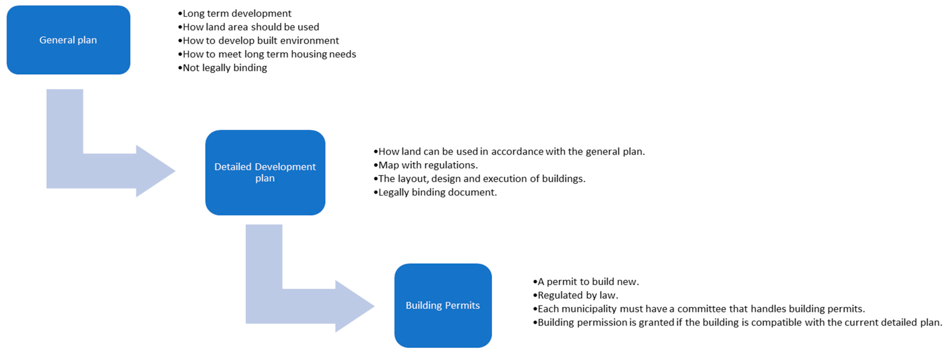
The relationship between land use policies and building permits can be described as regulation and compliance. Land use policies in Sweden provide a framework for the responsible use and development of land within each jurisdiction, while building permits serve as a tool for local governments to ensure adherence to these policies. The connection between the two runs through the development of municipal plans, from general plans to detailed development plans, which outline the long-term goals and direction for the municipality’s land use.
These plans, shaped through a collaborative process between local authorities, politicians, and citizens, consider a wide range of factors, including the optimal use and preservation of the built environment, housing needs, sustainable development goals, national interests, and environmental quality requirements. In metropolitan regions, regional plans are created to act as a principal guide for the municipality’s general plans. Although the general plan is not legally binding, it provides a clear vision for future land use.
The general plan provides an overview of the municipality’s land use goals and direction, while the detailed development plan is a more specific and legally binding document that governs the building permit process. Land use policies, such as zoning codes, regulate the types of land use allowed in different areas of the jurisdiction. These policies aim to control and manage growth, promote compatibility between different types of development, and preserve communities’ character. For example, a residential zone may only allow single-family homes, while a commercial zone may allow businesses and multistory buildings.
The detailed development plan, which includes a plan map and associated regulations, is the legally binding document that guides the building permit process (
Nyström 1994). It is part of the physical planning of the city adopted by the municipality management (
Olerup and Snickars 2017). The detailed development plan governs what can be built on a specific piece of land such as whether the land is intended for housing, offices, or a park. It also states whether the land is to be developed with, for example, multifamily or single-family houses, as well as restrictions on how the buildings may be designed, placed, and constructed. Thus, the detailed development plan outlines the specific land use designations for various parts of the municipality and ensures that new construction and development align with the broader land use policies and goals. The connection between land use policies and building permits in Sweden is crucial for responsible and sustainable land use and development. The combination of general and detailed development plans provides a comprehensive framework for regulating and compliance with new construction and development projects.
The issuance of building permits is a key component of Sweden’s land use and development process. When an individual or organization intends to construct a new building or make significant alterations to an existing structure, the individual or organization must first obtain a building permit from the local government. It is important to note that building permits are issued by the municipality (
Francart et al. 2019) after building permit documents have been tested against current national requirements and local regulations regulated in the Planning and Building Act (
Granath Hansson 2017;
Meijer et al. 2002). A building committee handles building permit issues in the municipality (
Meijer et al. 2002).
Therefore, the building permit process is a critical mechanism that enables local governments to enforce their land use policies and ensure that new developments align with broader community goals. Before a permit is issued, the proposal is thoroughly reviewed to determine its compliance with existing land use policies. The requirement of a building permit before new construction or significant alterations can begin is a safeguard for the responsible use and development of land within each jurisdiction. It gives local governments the authority to enforce land use policies and promote the community’s overall well-being.
As a result, land use policy and building permits are closely linked because land use policy sets development rules and standards, while building permits ensure that those rules and standards are observed in practice. The interaction between the land use policy, general plan, detailed development plan, and building permits is visualized in
Figure 1.
In summary, a building permit means that a new building meets the requirements set in the detailed development plan and the requirements of the Planning and Building Act. This implies that the municipality can control the number of building permits (even if no building permit caps are used) and that this control occurs through requirements and restrictions in the detailed development plan. Research also indicates that land use regulation reduces the number of building permits (
Jackson 2016). Our interpretation of this process of obtaining building permits via the detailed development planning process means that building permits per capita might be considered a good approximation for the municipality’s policy on land use. Furthermore, we scale the number of building permits on a per capita basis to control for differences in population size. The growth of building permits is likely to reflect a mix of supply and demand forces, and therefore, it might be considered as a measure of local restrictions as an alternative to indices of regulation constructed by using survey data. A growing number of building permits per capita is likely to reflect how well the local authorities comply with the expected growth of the urban population, while a decrease in this number might indicate an increased level of control over urban growth.
4. The Theoretical Model
We follow
DiPasquale and Wheaton’s (
1994) theoretical framework for housing market equilibrium. They emphasize that the general approach in theoretical studies with no capital constraints is that the demand for owner-occupied housing should depend only on the relative annual costs of owning as opposed to renting. However, in most empirical studies, demand depends separately upon price levels, interest rates, and average rents (
DiPasquale and Wheaton 1994). The long-term housing demand,
, can be expressed as a function of price,
Pt, and a set of demand variables,
Xt:
where subscript
t is the time period.
The long-term equilibrium stock,
, is expressed as a function of price,
Pt, and exogenous variables,
Yt:
DiPasquale and Wheaton (
1994) note that if
is measured in units, the demand function in Equation (1) reflects household formation decisions as well as tenure choice. Alternatively, if
is measured in money units, the demand function combines decisions about not only household formation and tenure choice but also the consumption of housing services.
In contrast to
DiPasquale and Wheaton (
1994), we apply a model that measures the
as the average size of housing units in the new construction of apartments. In other words, we descale the total number of square meters in new construction on an aggregate level to the number of square meters of the average housing unit in new construction, which reflects the number of square meters supplied in newly constructed units per household/ housing unit. A long-run equilibrium in the housing market is described as follows:
where
is equal to supplied quantity and
is equal to the demanded quantity. We transform Equation (3) in such a way that in our model,
is equal to the average size of the supplied housing unit (apartment) and
is equal to the average size of the demanded housing unit (apartment). Thus, following the approach used by
Warsame et al. (
2010), we have the following:
where
P is equal to price,
X1 is equal to other positive demand determinants such as the growth of population and disposable income, and
X2 is equal to negative determinants such as the growth of mortgage interest rates.
Y1 is equal to negative supply determinants such as the growth of land prices and construction costs, and
Y2 represents positive supply determinants such as the growth of rents and prices in the housing market. In equilibrium, the quantity demanded is equal to the quantity supplied. Given this model, we would like to find the price,
P*, at which the market is in equilibrium,
:
which can be written as follows:
Rearranging for price,
Pt, we obtain the following:
If
Pt = P*, then by inserting (7) into (4a) and solving for equilibrium between supply and demand,
Q*, we obtain the following:
We perform further mathematical rearrangements of Equation (8):
Finally, after all transformations performed in Equation (9), we obtain Equation (10), which represents Equation (8) in a short form:
where
All estimations in this paper are based on Equation (10).
5. Empirical Model and Data
5.1. Empirical Model
Our model analyzes long-run demand and supply for new apartments in Stockholm, Gothenburg, and Malmo—the three major urban regions in Sweden (see
Figure 2). A socio-economic description of these regions is presented in
Table 1.
Sweden is one of the countries that is experiencing a housing shortage due to a range of factors including rapid urban growth and a relatively low level of residential construction. About 83 percent of the counties in Sweden reported a shortage of housing in 2019. Around 94 percent of the Swedish population resides in those counties (
Swedish National Board of Housing, Building and Planning 2019). The situation is more difficult in larger urban regions such as Stockholm, Gothenburg, and Malmo, where it takes up to between 8 and 12 years longer to obtain a rental apartment in the inner city than it does in small and medium-sized cities (
The Stockholm Housing Agency 2018). This creates certain problems for different migration groups such as young people, labor migrants, divorced and single parents, and low-income households. The analysis conducted in the
Region Stockholm (
2018) report reveals differences in the migration flows between various age groups. The major group that moves to large urban regions is the “young adults”, i.e., people 18–29 years old. More than half of this group moved from one residence to another during the period of 2014–2016. At the same time, the absolute majority of older people live in the same house, and only ten percent of them move. The major migration flows normally occur into or within the same region (
Region Stockholm 2018).
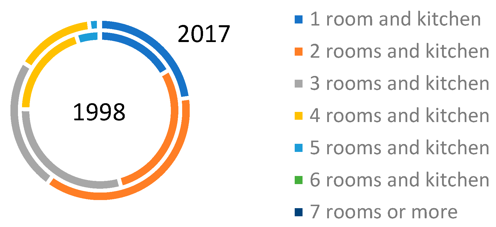
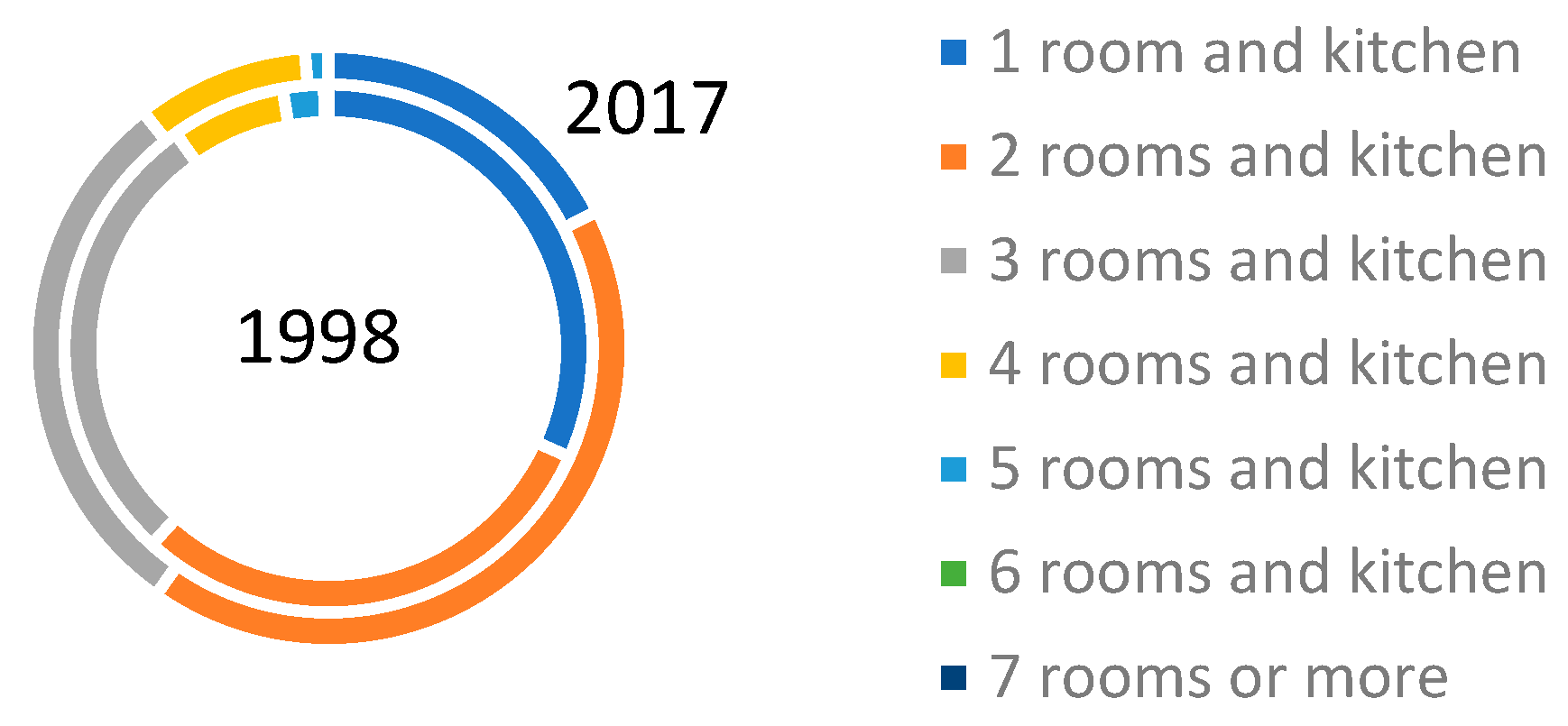
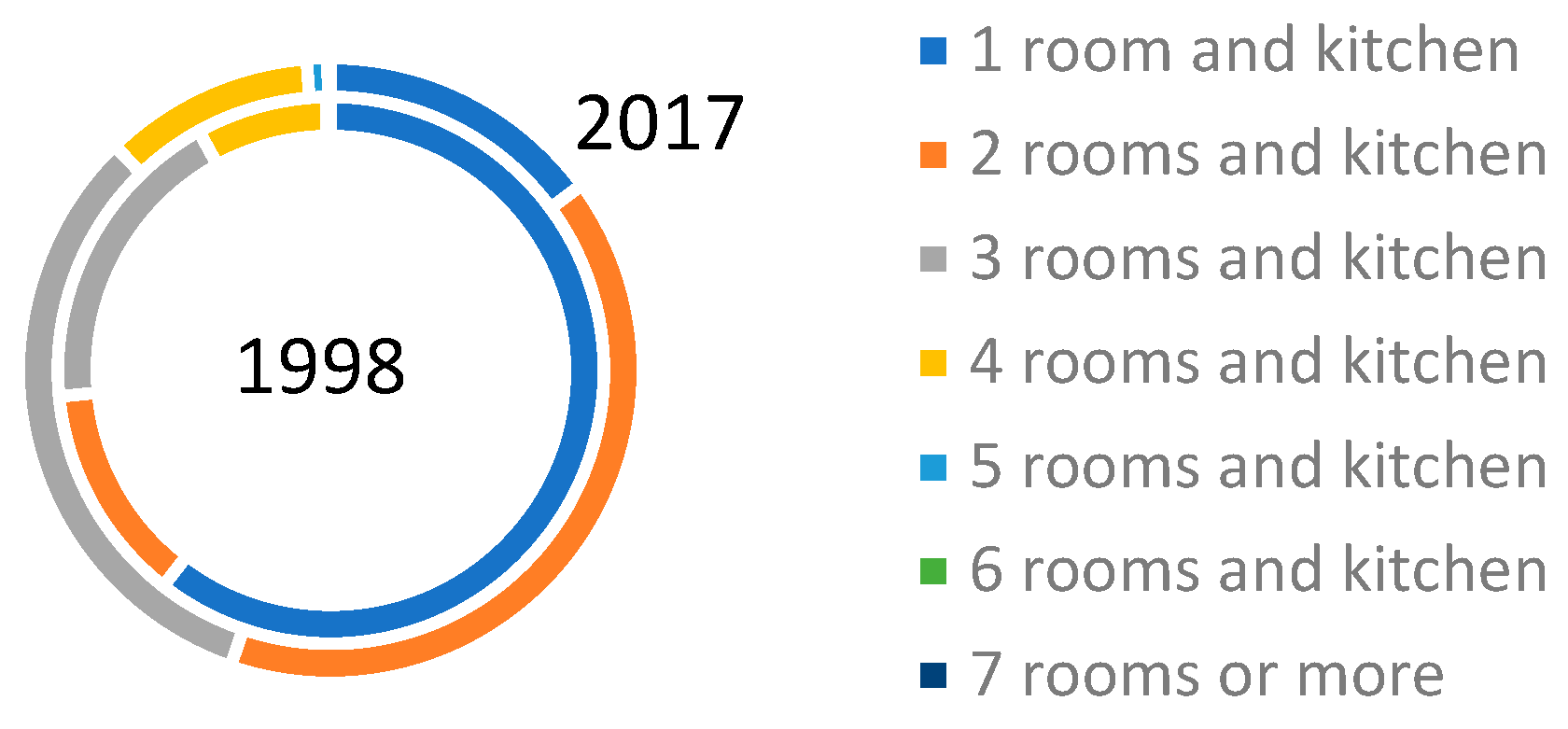
According to data from SCB Statistics Sweden, construction activity in larger urban agglomerations is in tandem with demographic trends, with a slight trend towards a slowdown in recent years. In other words, supply seems to be in line with population growth, the number of people per dwelling unit has not varied significantly in the last two decades, and the average household size is quite stable in major Swedish urban regions. For example, the number of people per dwelling unit was 2.09 in 1995 and 2.07 in 2019. The average household size was 2.1 persons per household in Stockholm and 1.9 in the Gothenburg and Malmo urban regions during 2012–2022. (Source: SCB Statistics Sweden, own calculations). However, the share of “smaller apartments” (in terms of the number of rooms in the apartment) in new construction has increased in recent years. Of all new apartments, 6 out of 10 are two-room apartments or smaller, while the share of similarly sized apartments in the existing stock is about half of the total apartment stock. There is a notable difference in housing tenure forms as more rental apartments are built as “small apartments” in comparison to those in the housing cooperative sector. Only 5 percent of all newly constructed apartments have five rooms or more, which is smaller in comparison with the share of apartments of similar size in the existing stock. The typical apartment built in both the rental and housing cooperative sector has two rooms and a kitchen (
Region Stockholm 2019). The structure of new construction of apartments by type in three Swedish regions in 1998 and 2017 is presented in
Figure 3,
Figure 4 and
Figure 5. The size of each piece on the diagram communicates the proportion of each apartment’s type in the size of the total new construction of apartments as a whole. As can be seen from
Figure 3,
Figure 4 and
Figure 5, the largest share of new apartments in Stockholm in 2017 belongs to one- and two-room apartments with a kitchen, while in Gothenburg and Malmo, it is two- and three-room apartments with a kitchen. In 1998, the distribution looked slightly different, with a larger share of two- and three-room apartments in new construction in Stockholm, one- and two-room apartments in Gothenburg, and one-room apartments in Malmo.
The size of the multifamily housing segment in the total housing stock in three major urban areas in Sweden varies between 63 and 74 percent in 2018. The cooperative apartment segment contributed to 35–53 percent of the multifamily housing stock; the rest is rental apartments. The share of condominiums in multifamily housing in larger urban areas in Sweden is less than 0.03 percent, and therefore it is neglected in this study. The share of the single-family housing segment in housing stock varies between 24 and 35 percent depending on the city, but it stays relatively constant in each city over the long run (SCB Statistics Sweden, own calculations).
The size of the multifamily housing segment in new construction in three major urban areas in Sweden varied between 33 and 85 percent in 2018. The share of multifamily housing construction was less than 50 percent only in one out of three areas and only during 11 out of 20 years of the period (SCB Statistics Sweden, own calculations). Thus, the apartment segment represents a major part of the total housing stock in large metropolitan areas in Sweden; therefore, the analysis in this study has a main focus on it.
The model divides the housing sectors into renter-occupied and cooperative housing since these two are the major forms of housing tenure for the apartment segment in Sweden. These two subsectors are interconnected and affect each other in two ways. The price of renting an apartment in comparison to buying affects the number of households that rent or buy new apartments. The total demand for urban land depends on the total demand for new apartments in each subsector. The system of equations representing these subsectors represents these markets in our model of the urban housing sector.
The aggregate tenant demand in the rental sector depends on the growth of the population (renters), the price of rental housing services relative to the price of other goods, and average disposable income. The aggregate tenant demand in the housing cooperative sector depends on the growth of population (potential buyers looking for a new apartment), price per square meter relative to the price of other goods, average disposable income, and mortgage interest rates. Though there may be some differences in the factors mentioned above, for example, differences in the average income or preferences in the type of housing for a certain population, this formulation of the fundamental factors affecting demand and supply in the rental and housing cooperative sectors is in line with previous studies in the literature review.
Land is an essential component in the provision of housing services, and its supply is not elastic. In the market, investors (or property owners) demand rental and housing cooperative properties, and property developers build them. The aggregate long-run supply of rental and housing cooperative properties depends on the investment values of real estate land prices and other components, such as the price for building materials and wages for construction workers. Therefore, we include land prices as a direct measure of municipal land policies in our model. An alternative could be to include the gap between housing prices or rent and land prices as an indirect measure of municipal land policies. A similar indirect measure as an approximation of regulation is used in the study conducted by
Glaeser et al. (
2005). In their study, they emphasize that since the degree of housing market regulation is difficult to measure, an alternative approach based on the neoclassical economic theory of perfect competition might be used. This theory predicts that competition among builders will ensure that prices equal average costs. In unregulated markets, building heights will rise to the point where the marginal cost of adding an additional floor equals average costs (which will equal the market price). If market restrictions limit the size of a building, free entry of firms still will keep the price equal to the average cost. Thus, the key difference between a regulated and an unregulated market is the gap between prices and marginal costs.
Glaeser et al. (
2005) use this difference to measure the extent of housing supply restrictions.
One more component to be added to the model as a direct measure of regulation is the number of building permits per capita. As emphasized earlier, it works as a proxy for more/less permissive types of building policies in the municipality.
5.2. Modeling Approach
We follow the standard econometric methodology and focus on the estimation of a set of equations with panel data. Our dataset contains data for three major urban areas in Sweden on an annual basis for a 20-year period and covers new construction in both the rental and housing cooperative markets. In this way, we intend to estimate the equations jointly to allow cross-equation restrictions to be imposed or tested and to gain efficiency, since we expect the error terms across equations might be contemporaneously correlated. Such equations are often called seemingly unrelated regressions (SUR), as proposed by
Zellner (
1962).
According to
Wooldridge (
2009), the SUR estimator is used if the number of units, N, is small, as it is in our dataset (for example, N < 10). Examples of SUR equations might be a set of demand equations across different sectors, industries, or regions.
Zellner’s (
1962) approach is simplified since it captures the efficiency due to the correlation of the disturbances across equations. It matches well with our dataset since there may be factors that affect the dependent variable (average size of apartment) jointly in both the rental and housing cooperative sectors, and we expect that the error terms across equations may be correlated. Thus, the joint set of equations for SUR estimations in Equation (10) will be as follows:
where
is the equilibrium size of an apartment in new construction in the rental sector,
is the same for the housing cooperative sector,
is the error term for the rental sector equation, and
is the error term for the housing cooperative sector equation.
5.3. Data Description
The dataset comprises annual data for several variables in three major urban areas in Sweden (Stockholm, Gothenburg, and Malmo) for 20 years, covering the period from 1998 to 2017. The majority of data come from SCB Statistics Sweden, except for variables such as price per square meter for apartments and single-family homes, which come from the company Mäklarstatistik, a company that collects data about transactions in the housing market in Sweden. Mortgage interest rate data come from Swedbank, which is one of four major banks in Sweden.
The number of building permits per capita is calculated as the number of building permits for the construction of multifamily buildings issued by the city council in each city as the total number of apartments to be constructed in multifamily buildings over the population within its area. All economic variables are transformed into real terms and then transformed into natural logarithms for regression analysis. The summary statistics are presented in
Table 2.
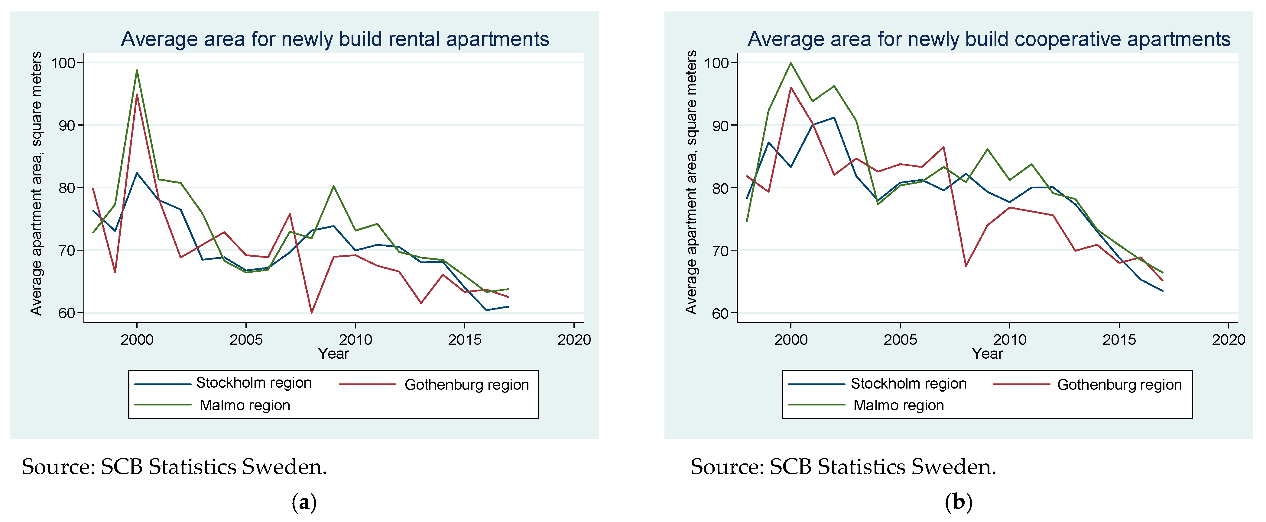
As is shown in
Table 2, the average apartment area is about 71 square meters and 80 square meters for newly built rental apartments and cooperative apartments, respectively. The average apartment area fluctuated during the study period between 60 and 99 square meters for rental apartments and between 64 and 100 square meters for cooperative apartments with standard deviations of 7 and 8 square meters, respectively.
Figure 6 presents the long-run dynamics of the average apartment area. The decrease in the average area was higher for rental apartments and lower for housing cooperatives.
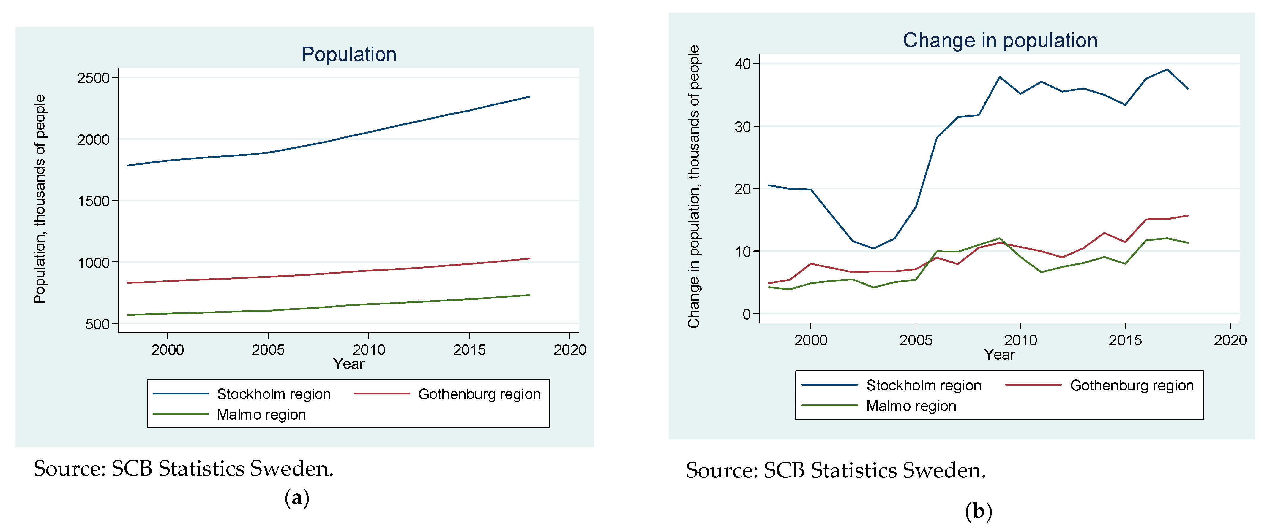
Figure 7 presents the population dynamics during the study period. The annual population change in major Swedish cities is plus 14,739, which is 1.2 percent growth in the average population within these areas.
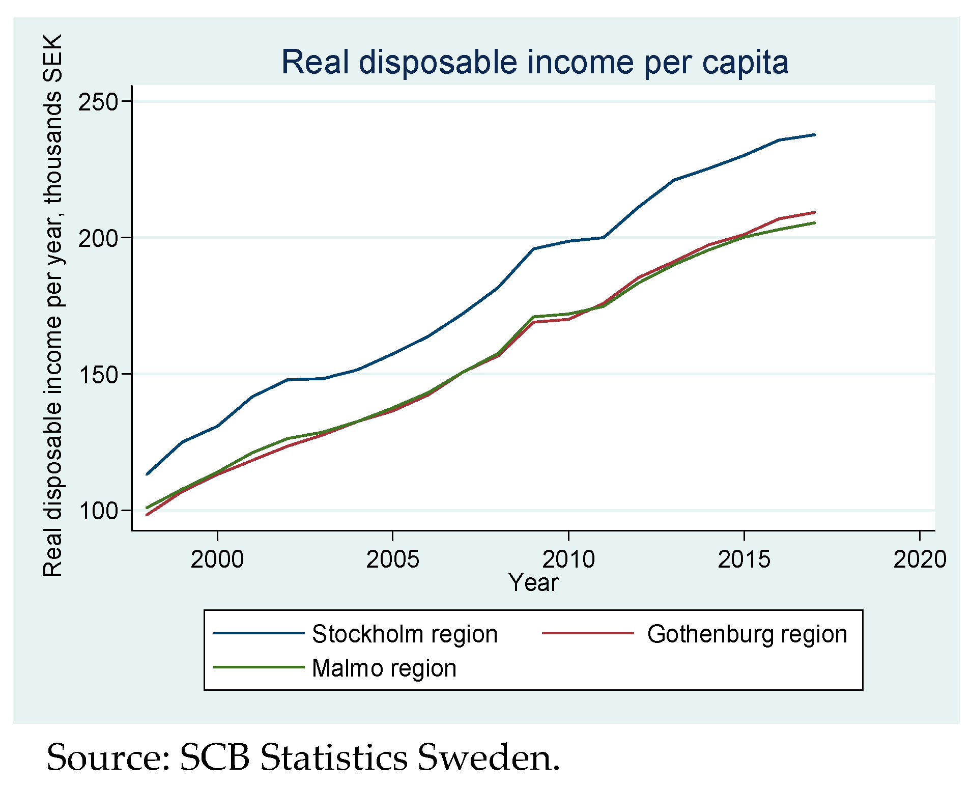
The average disposable income is SEK 164,000 per year, with a standard deviation during the study period of SEK 37,600 (see
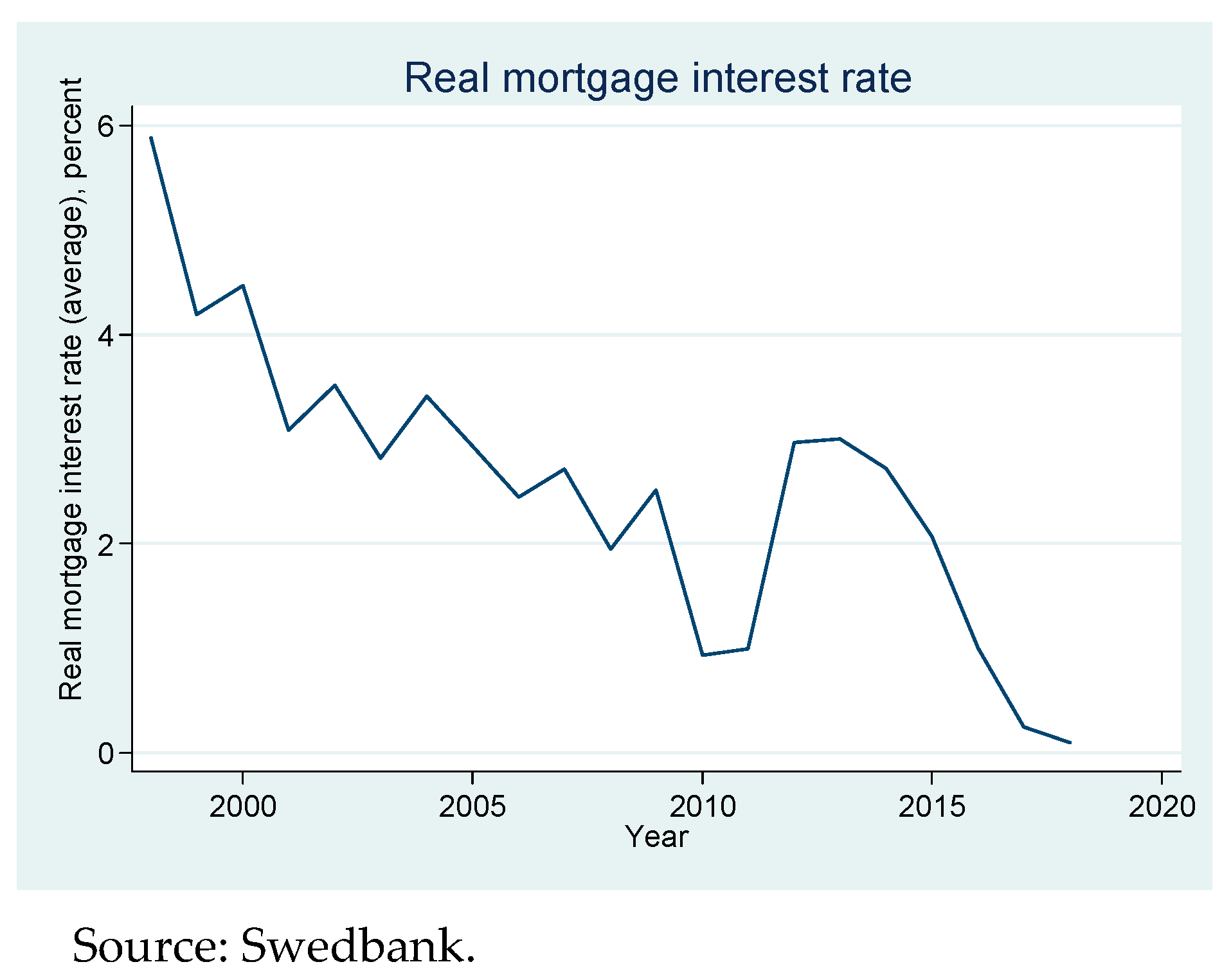
Figure 8). The average mortgage interest rate is about 2.69 percent, with a minimum of 0.3 percent, a maximum of 5.9 percent, and a standard deviation of 1.3 percent during study period (see
Figure 9).
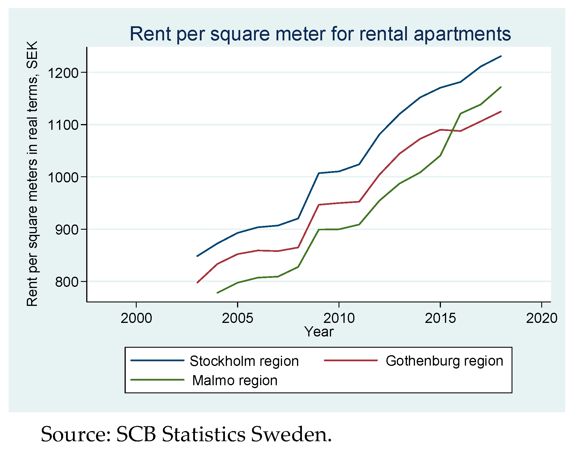
The average real annual rent during the study period is SEK 968 per square meter with a standard deviation of SEK 121 per square meter (see
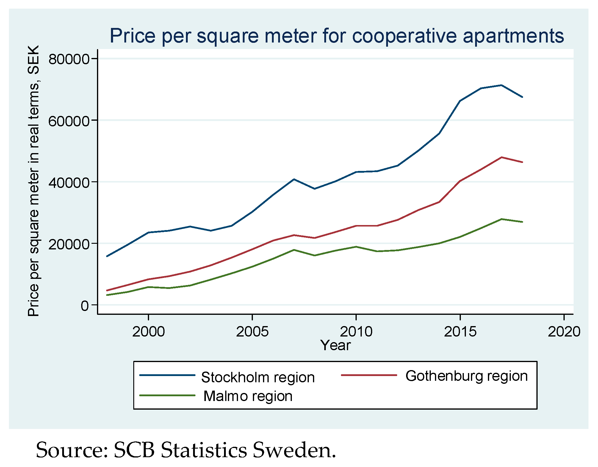
Figure 10). The average real price per square meter during the study period for housing cooperatives is SEK 25,498 per square meter with standard deviation of SEK 16,300 per square meter (see
Figure 11).
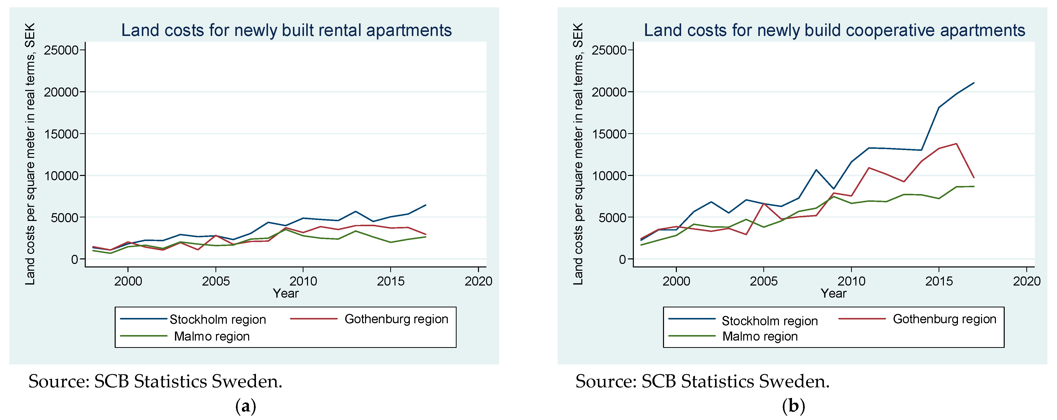
The average land cost per square meter for newly built rental apartments is SEK 2767, which is 2.7 times less than that for cooperative apartments, which is SEK 7454 per square meter (see
Figure 12).
The average number of building permits for multifamily buildings expressed as the number of apartments to be constructed is 3711 per year, which contributes to 0.0028 building permits per capita on average or 2.8 building permits per 1000 inhabitants during the study period (see
Figure 13).
5.4. Pre-Test of Data
Macroeconomic data are often non-stationary, with means, variances, and covariances that change over time. We follow the standard econometric procedure by first checking the data for stationarity.
Im et al. (
2003) developed a set of tests for testing unit roots in panel data. The Im–Pesaran–Shin (IPS) test relaxes the assumption of common autoregressive parameters such as cultural and institutional factors. Moreover, the IPS test does not need balanced datasets. Since property market dynamics depend very much on location, this test is the most appropriate for the type of data we have.
Table 3 presents the results obtained from the stationarity test.
Results reveal the non-stationary character of such variables as population and change in it, real mortgage interest rate, and rent per square meter in real terms. Regression models for non-stationary variables might give spurious results. In order to obtain consistent, reliable results, the non-stationary data were transformed into stationary data by taking the first differences on variable levels.
The results show that all first-difference variables are integrated of order 0; that is, all variables are stationary. Therefore, in regression estimations for Models 1 and 2 below, the dependent variable average apartment area in newly built apartments is taken in levels, while all independent variables except building permits per capita for multifamily buildings are taken as first differences.
6. Results and Discussion
6.1. Regression Results
We adjust for small sample size and estimate the Breusch–Pagan value for independent equations. The default is the two-step SUR estimation (Model 1). Because SUR estimation reduces to OLS if the same set of regressors appears in each equation (
Cameron and Trivedi 2009), we omit some variables from the first equation for the rental sector and other variables from the second equation for the housing cooperative sector (Model 2). We estimate the correlation matrix for the fitted residuals that are used to form a test of the independence of the errors in the two equations. The results from the SUR estimations are presented in
Table 4.
We have obtained the following results for Model 1: A test of the joint significance of all regressors in the equation has a value of 49 percent with a p-value of 0.000 for the rental sector and 54 percent with a p-value of 0.000 for the housing cooperative sector.
The most influential factor affecting apartment size in new construction in both the rental and housing cooperative sectors is the growth of real disposable income. One percent increase in real disposable income growth corresponds to a 1.6 percent larger average apartment area in newly built rental apartments and a 1.2 percent larger average apartment area in new housing cooperative apartments. Change in population growth is significant for apartment size in the rental sector but not in the housing cooperative sector. This might be evidence of the population densification process that occurs in the rental sector of the housing market. One percent increase in population growth leads to a 0.09 percent decrease in the average apartment area in newly built rental apartments.
Model 1 demonstrates that changes in real mortgage interest rates, real rent levels for rental apartments, and real price per square meter for housing cooperatives do not affect the apartment size in new construction in the rental sector. In a similar way, change in the real price per square meter does not affect the apartment size in new construction in the housing cooperative sector. A higher decrease in real mortgage interest rates and growth in real rent per square meter have a negative impact on apartment size in the housing cooperative equation. Both of these estimators are significant. This implies that a one percentage point decrease in mortgage interest rate leads to a decrease in the average apartment size by 0.04 percent. One percent higher real rent growth per square meter leads to a decrease in average apartment area in the housing cooperative sector by 1.19 percent.
Changes in real land costs per square meter and changes in building permits per capita both have negative impacts and are significant for rental and housing cooperative sector equations. Growth in real land costs per square meter by one percent decreases the average apartment area by 0.04 percent in newly built rental apartments and by 0.06 percent in cooperative apartments. An increase in the number of building permits per capita (as the number of apartments to be constructed per capita) by one percent is associated with a decrease in average apartment area by 0.05 percent in newly built rental apartments and 0.08 percent in housing cooperative apartments.
The errors in the two equations positively correlated with a correlation coefficient of 86 percent. The correlation is strong; therefore, the efficiency gains in SUR estimation are substantial. The Breusch–Pagan test of error independence indicates a statistically significant correlation between the errors in the two equations, as should be expected given that the two categories of the average size of the apartment may have similar underlying determinants. This implies that the regression-by-regression results are consistent.
Model 2 is estimated without insignificant factors from Model 1. The overall results for Model 2 indicate that we explain approximately 48 percent of the variation in the apartment size in newly constructed residences in the rental sector. On the other hand, estimation results explain approximately 53 percent of the variation in the average apartment size in the housing cooperative sector. Hence, it seems that the fundamental variables explain the variation in apartment size better in the less regulated market than in the more regulated market, i.e., the rental sector where the rents are subject to rent control. The Breusch–Pagan test of error independence indicates a statistically significant correlation between the errors in the two equations. This implies that SUR estimation is efficient.
Model 2 explains the variation in apartment size across the regions and over time. The results demonstrate that all fundamental variables used in Model 2 are significantly different from zero in the equations for both sectors. The estimated parameter concerning the effects of the change in population on the size of the rental apartment is significant and negative. One percent change in population growth leads to a 0.1 percent decrease in the average apartment area in newly built rental apartments. However, growth in real disposable income leads to construction of larger apartments in both sectors. One percent higher growth of real disposable income corresponds to 1.5 percent higher average apartment area in newly built rental apartments and 1.1 percent higher average apartment area in new housing cooperative apartments.
Adverse effects of change in real land prices and building permits per capita were observed for average apartment size in both sectors. Higher growth in real land costs per square meter by one percent decreases the average apartment area by 0.04 percent in newly built rental apartments and by 0.06 percent in new housing cooperative apartments. Higher growth in real land prices causes developers to build smaller apartments. These negative effects have a larger impact on housing cooperatives in comparison with the regulated rental sector.
The building permits per capita variable is significantly different from zero, indicating that building permit regulations are important, although the effect is negative. The negative sign of this estimator provides evidence that downsizing in housing development occurs even if the number of building permits per capita is growing in relation to population size. An increase in the number of building permits per capita (expressed as the number of new apartments to be built per capita) by one percent is associated with a decrease in average apartment area by 0.05 percent in newly built rental apartments and by 0.08 percent in new housing cooperative apartments.
If we analyze the results from the cooperative housing market in Model 2, we can observe that the change in the real interest rate has a positive impact on constructed apartment size. Real interest rates have decreased in recent decades, and real housing prices have increased considerably, which resulted in the building of smaller cooperative apartments. Estimation results reveal that a one percentage point decrease in mortgage interest rate decreases the average apartment size by 0.04 percent. Rent levels are related to apartment size; that is, higher growth in real rent per square meter is associated with smaller apartments in new construction of housing cooperatives. One percent higher growth of real rent per square meter leads to a decrease in average apartment area in newly built housing cooperatives by 0.9 percent.
It is difficult to relate results from Models 1 and 2 directly to previous studies that analyze downsizing in residential development and use the size of housing units as the subject of analysis. These studies utilize surveys as the main method of data collection and conduct analysis with limited application of logistic regressions. Indirectly, our results might be related to other studies that use the number of dwelling units as a dependent variable and measure of new housing supply. Our regression estimations have similar signs. An increase in real disposable income and population growth has a positive effect, as found by
Warsame et al. (
2010) and
Engerstam et al. (
2022), while a negative effect is observed for growth in real rents (as found by
Riddel (
2004)), interest rate (as found by
Wigren and Wilhelmsson (
2007)), and land prices (as found by
Lerbs (
2014)).
6.2. Testing for Granger Non-Causality in Panel Data
In addition, we tested the stability of relations between dependent and independent model variables by applying the panel Granger non-causality test approach developed by
Juodis et al. (
2021). This test offers a size and power performance superior to that of existing tests of Granger causality in panel data. The test has two other useful properties: (1) it can be used in multivariate systems; (2) it has power against both homogeneous and heterogeneous alternatives. Results of the joint and univariate half-panel jackknife (HPJ) estimators with computed cross-sectional heteroscedasticity-robust variance are presented in
Table 5.
Results of the test demonstrate that the null hypothesis of Granger non-causality is rejected for all independent variables in the equations for the rental sector and housing cooperative sector either at joint or individual test levels depending on number of lags applied. This implies that past values of independent variables in the model help to predict average apartment size as the dependent variable in the model over and above the information contained in the past values of it.
6.3. Discussion
As the results demonstrate, land and building permit policies do contribute to a gradual decrease in average apartment size over the long term. We can observe these effects for both the rental and housing cooperative subsectors of the housing market in the three largest urban regions in Sweden.
Despite the fact that new construction contributes each year only to about 1–2 percent of the total housing stock and therefore cannot be considered a significant change in the structure of the housing market, the impact of these changes is not to be neglected. Moreover, new residential construction and economic indicators, such as prices or rent levels, affect the existing housing stock through spillover effects and play an essential role in providing the information needed for evaluating this development and analyzing the current state of the housing market.
As presented in the results of this paper, the most influential factor affecting the size of apartments in new construction in both the rental and housing cooperative sectors is the change in real disposable income. This effect is positive; i.e., the higher the growth in real disposable income, the higher the average apartment area demanded by the end consumers of the housing goods. A decrease in real disposable income is associated with a smaller average size of the apartments in new construction.
What will the implications of this process be if current conditions persist in the future? Average dwelling size and quality change over time. The housing market has been operating in a low-interest-rate environment in recent decades, which implies that it is becoming somewhat cheaper to finance the purchase of land and new construction for property developers. However, this situation does not lead to a gradual increase in housing supply, but rather a decrease in the size of the final product of construction (i.e., apartment dwellings). This in turn creates an environment where house prices do not fall over the long term due to the lower elasticity of housing supply, and since mortgage loans finance housing, we can instead observe growth in household debt. Thus, a new dwelling unit is becoming somewhat smaller with time, but relatively less affordable over the long run. This creates mismatches between the supply of dwellings coming from construction and the demand for them that is represented by requirements for living space from different population groups.
Another important implication is that a decrease in apartment sizes leads to an increase in the density of the population in large urban regions. This might have negative socio-economic consequences, such as overcrowding and a higher risk for socio-psychological problems.
7. Conclusions and Policy Implications
Rapid population growth within metropolitan areas in Sweden has put pressure on sustainable housing provision in many municipalities and become a topic of intense interest for academicians and policymakers. Although research on new housing construction has been recognized as important, it lacks studies that examine the impact of land and building policies on the size of the new multifamily housing units. If restrictions on building permits and land policy mean that what is being built is smaller, the socio-economic efficiency will also be affected, and there is a risk that welfare losses will arise. Therefore, this study contributes to existing research by deepening the understanding of the effects of land and building policies on new residential supply.
Previous studies on new residential supply focus on the number of new housing units constructed. The number of building permits issued by a municipality is used in some cases as a measure of housing starts. We apply a different approach to analyze the dynamics of new residential construction and utilize the average apartment size as a subject of analysis. This approach allows us to evaluate new construction from both the societal and planning perspectives since changes in the average apartment size might be a result of both the municipal policies and the preferences of households. The average apartment size in new construction might tell us whether there might be a risk for increased overcrowding, a situation in which fewer different population groups will be able to find appropriate housing for their needs. Moreover, the dynamics of average unit size might help in evaluating changes in the structure of the housing market on an aggregate level and determining if, for example, downsizing in new construction occurs. Previous studies on housing downsizing apply survey methods investigating different moving options, reasons for downsizing, and desires and preferences of households at the micro level. We, in distinction from previous research, consider the size of the housing unit at the macro level by applying seemingly unrelated regressions on construction of rental and cooperative apartments in the three largest urban regions in Sweden.
In line with the main objectives of this paper, we can draw several conclusions. The primary factor that affects the size of new apartments in new residential construction in the three largest Swedish regions is disposable income. The effect is positive and strong in comparison with other fundamentals. However, we can conclude that the main factors that bring adverse effects and contribute to the downsizing of the final housing product are land prices and building policies. The more expensive the land allocated for residential construction is, the smaller the apartment sizes will be over the longer run. We expected that restrictive building policies would contribute positively to downsizing the apartment area since developers that operate in an environment with building constraints would compensate for high land prices by sacrificing the size of the final housing goods produced. Our results demonstrated the opposite. High land prices are probably an artifact of regulation and not purely a result of exogenous demand-side factors. Many restrictions on where multifamily development can occur could plausibly be driving up the cost of land for multifamily projects.
Several implications arise from this study: In a market with building policy restrictions and growing land prices, the housing market will react by downsizing the final product to the consumer instead of decreasing the price per square meter. This implies deviations from socio-economic development in housing markets in the long run, which occurs through short-term adjustments in construction. Moreover, unregulated markets, such as the cooperative housing sector in Sweden, react more strongly to these changes in comparison to a regulated market, such as the rental apartment sector in the Swedish housing market. Therefore, building policies are to be formulated and applied in a way that prevents such deviations from socio-economic development in the long run.
Even though this study was conducted in a Swedish context, the results have implications for other countries. For instance, it might be of interest to investigate if differences in institutional settings related to municipal land use and building policies affect the size of dwelling units in new residential construction in other countries in another way.
This empirical study has analyzed apartment size in new construction in both rental and housing cooperative sectors, but it does not address a potential consumer shift between different types of dwellings. As apartments in the rental sector on average tend to be smaller than those in the ownership sector, a larger shift from the housing cooperatives to rental apartments would likely contribute to reducing the average size.
Future research could also address challenges to the housing market that might result from downsizing. For example, additional research could investigate how downsizing can accommodate people in different life situations.
Some other issues of interest are as follows:
Relocation decisions of younger and older households—why do they move and not move?
Gender issues in relation to housing size (for example, whether women’s tendency to downsize is larger than men’s).
Providing further insights into these issues will help policymakers to make the most informed decisions and thereby improve new residential supply so that it is able to meet the needs of different population groups.


