Explaining Deep Learning Models for Credit Scoring with SHAP: A Case Study Using Open Banking Data

Abstract

Predicting creditworthiness is an important task in the banking industry, as it allows banks to make informed lending decisions and manage risk. In this paper, we investigate the performance of two different deep learning credit scoring models developed on the textual descriptions of customer transactions available from open banking APIs. The first model is a deep learning model trained from scratch, while the second model uses transfer learning with a multilingual BERT model. We evaluate the predictive performance of these models using the area under the receiver operating characteristic curve (AUC) and Brier score. We find that a deep learning model trained from scratch outperforms a BERT transformer model finetuned on the same data. Furthermore, we find that SHAP can be used to explain such models both on a global level and for explaining rejections of actual applications.

1. Introduction

The introduction of open banking APIs under the European Payment Services Directive (PSD2) has opened up a new source of credit behavior information for potential bank customers, previously only accessible to their current banks. This increased data availability for competing banks, which includes daily balances, transaction amounts, and textual descriptions of customer transactions, has the potential to significantly increase the performance of application credit scoring models and, thus, impact competition in the lending market. Given this new landscape, it becomes even more crucial for banks to develop more accurate and efficient credit scoring models to maintain their market share and offer better services to customers.

This study is motivated by the need to investigate and understand the predictive value of this data source, specifically textual descriptions from customer transactions accessible through open banking APIs. By developing credit scoring models using state-of-the-art deep learning techniques based on these textual descriptions, banks can potentially leverage this information to more accurately assess the creditworthiness of potential customers, leading to better lending decisions and reduced credit risk.

In addition, when using deep learning methods, it becomes increasingly important to provide interpretable explanations for the credit scoring models, ensuring fair and transparent credit decision-making and abiding by strict regulations. By examining the applicability of SHAP as a tool for explaining predictions from deep learning models developed on textual descriptions from customer transactions, this research aims to contribute to the understanding of model interpretability in the context of credit scoring.

The purpose of this study is, thus, to examine the predictive value of textual descriptions from customer transactions available through open banking APIs when developing state-of-the-art deep learning-based credit scoring models, and to examine whether SHAP can be a useful tool when explaining predictions from such models.

We explore the following research questions: (1) Are textual descriptions from customer transactions available through open banking APIs predictive of future defaults among a bank’s retail customers? (2) Can SHAP be used to explain predictions from state-of-the-art deep learning models developed on textual descriptions from customer transactions?

To answer our research questions, we create credit scoring models using deep learning and natural language processing (NLP) techniques on textual descriptions of bank customer transactions available through open banking APIs. We evaluate the predictive performance of these models using the area under the receiver operating characteristic curve (AUC) and Brier score. We then use SHAP to explain the predictions made by these models, particularly examining which words contribute the most to high-risk (score) predictions.

We find that a deep learning model trained from scratch on text strings from open banking data outperforms a BERT transformer model finetuned on the same data. Furthermore, we find that SHAP can be used to explain such models both on a global level and for explaining actual rejections of loan applications.

Our main contribution is exploring how SHAP can be applied in banking to interpret and understand predictions from state-of-the-art deep learning models trained on raw transaction data available through open banking APIs. We also contribute by showing that training a deep learning model from scratch results in a better performing model than using a transfer learning approach based on a multilingual BERT when the training data consists of concatenated text strings from transaction data.

The rest of this paper is organized as follows. In Section 1.1, we give an overview of the relevant literature on credit scoring, machine learning, and XAI. In Section 2, we describe the dataset. In Section 3, we describe the methods and models applied in the study. In Section 4 and Section 5, we present and discuss the results, respectively. Section 6 concludes and proposes ideas for further research.

1.1. Literature Review

In credit scoring, lenders calculate a score to measure the probability that a customer will default in the future as a basis for accepting or rejecting loan applications. Historically, logistic regression has been the most commonly used technique to calculate these scores in the banking industry (Thomas et al. 2017).

Well-established machine learning techniques have also proven to be successful in building credit scoring models. Some examples are k-nearest neighbor (Hand and Henley 1997; Henley and Hand 1996), neural networks (Desai et al. 1996; West 2000; Yobas et al. 2000), decision trees (Yobas et al. 2000), and support vector machines (Baesens et al. 2003). According to some studies, machine learning methods, including both single classifiers and ensemble models, outperform logistic regression in predicting defaults (Lessmann et al. 2015; Uddin et al. 2019).

During the past decade, more sophisticated machine learning models based on deep learning techniques have been shown to outperform traditional machine learning models, especially for unstructured data sources, such as audio, images, and text. In contrast to conventional machine learning models, where features are handcrafted from raw data by experts, deep learning models take data as inputs in raw form without any preprocessing or creation of variables. Two types of deep learning models have demonstrated state-of-the-art results: the recurrent neural network (RNN) and the convolutional neural network (CNN) (LeCun et al. 2015).

While CNNs have typically been considered state-of-the-art in image classification, RNNs have been crucial in advances in natural language processing (NLP). Historically, supervised learning has been the main learning approach used in state-of-the-art machine learning models in most classification tasks. Large databases with labeled images have been curated to act as the training basis for increasingly larger and more complex end-to-end deep learning models. Generally, the predictive performance of such models has increased with increasing access to labeled training data.

Furthermore, transfer learning has been an essential component in the widespread use of supervised deep learning models, especially for images. Transfer learning is a concept in which a predictive model developed for one task can be finetuned to another similar task (Howard and Ruder 2018). It is mostly beneficial when the training dataset has too few data points to train a full-scale model from scratch and can be seen as an optimization technique that usually improves model performance.

In contrast, only in recent years has NLP witnessed the introduction of models that genuinely utilize transfer learning. Important scientific contributions contributing to this development are the concept of attention (Chorowski et al. 2015), the transformer model architecture in 2017 (Vaswani et al. 2017), the bidirectional encoder representations from transformers (BERT) model in 2018 (Devlin et al. 2018), and the generative pre-trained transformer 3 (GPT-3) model in 2020 (Brown et al. 2020).

Although former state-of-the-art NLP deep learning models were mostly developed using supervised learning only, transformers are commonly pretrained using self-supervised learning on large quantities of unlabeled data to learn patterns about languages, both on a grammatical and semantic level. The use of pre-training addresses the shortage of large, labeled datasets for text. Once pre-training was introduced, NLP models were able to better grasp patterns within the language due to the huge amount of unlabeled data. It also allows anyone with access to these models to use the pre-trained model on similar but different tasks.

In credit scoring, most research involving deep learning techniques has focused on performance comparisons between deep learning models and conventional machine learning and statistical methods. These comparisons have mostly been made on the basis of publicly available, conventional, tabular datasets containing hand-made explanatory variables. Such studies include Hamori et al. (2018), Addo et al. (2018), and Gunnarsson et al. (2021). Generally, these studies show that ensemble models (e.g., gradient-boosting models) are superior in terms of prediction accuracy compared to deep learning models when these models are developed on conventional datasets containing hand-made explanatory variables.

Some researchers have investigated the effect of developing deep learning models on raw, unstructured, and unaggregated data in contrast to conventional credit scoring datasets. Examples are Kvamme et al. (2018), who developed a deep learning model based on daily balances from current accounts, Hjelkrem et al. (2022a, 2022b) and Ala’raj et al. (2022), who applied deep learning algorithms on financial transaction amounts, while Mai et al. (2019), Stevenson et al. (2021), and Kriebel and Stitz (2022) applied deep learning algorithms on raw text. Stevenson et al. (2021) successfully finetuned a BERT model for credit scoring and the Spanish language, focusing on small businesses. Kriebel and Stitz (2022) used a BERT model to extract user-generated text and show that text can significantly improve a credit scoring model based on peer-to-peer lending data. For a more detailed overview of the literature on BERT-based models, see, e.g., Acheampong et al. (2021).

These results indicate that when deep learning algorithms are trained on raw, unaggregated data rather than hand-made, aggregated explanatory variables, they outperform conventional machine learning models. This aligns with findings in other scientific fields, such as image processing, audio, and speech, where end-to-end deep learning has replaced conventional machine learning based on hand-made explanatory variables as state-of-the-art.

Still, while deep learning models have shown great promise in increasing performance for predictive models, they are considered black-box models. That is, it is impossible for humans to comprehend the inner workings of such models, which is crucial to fully understand their predictions. Consequently, the research field of explainable artificial intelligence (XAI) has emerged during the past decade, focusing on developing methods and techniques to explain the predictions of deep learning models (Adadi and Berrada 2018). Examples are LIME (Ribeiro et al. 2016), SHAP (Lundberg and Lee 2016), deepLIFT (Shrikumar et al. 2017), saliency maps (Itti et al. 1998; Simonyan et al. 2014), GradCAM (Chattopadhay et al. 2018; Selvaraju et al. 2017), guided backpropagation (Springenberg et al. 2014), and layer-wise relevance propagation (Bach et al. 2015).

The use of XAI is becoming increasingly important in the financial industry due to the complexity of machine learning models and the need to use them in a safe and understandable way that complies with regulations. Lending presents unique challenges for machine learning models because of the high stakes involved in daily decision-making. Both financial stability and consumer protection are important considerations. The use of deep learning models in credit scoring could pose a risk to financial stability if the underlying mechanisms of the models are not well understood, potentially leading to a financial crisis. At the same time, consumer protection is a key concern in the highly regulated financial sector. For example, under the EU General Data Protection Regulation (GDPR), consumers have the right to an explanation when they are subjected to automated decisions. As a result, the use of AI in credit assessment processes at banks is dependent on XAI techniques that can meet these regulatory requirements.

It is not yet clear which XAI methods and techniques are most suitable for use in credit scoring or if current state-of-the-art methods are able to meet the needs of all stakeholders in the financial industry. There is a lack of consensus on this topic in the literature and financial industry. However, Lundberg and Lee (2017) have shown that SHAP (Shapley additive explanations) is a unified local-interpretability framework with a rigorous theoretical foundation on the game theoretic concept of Shapley values (Shapley 1952).

SHAP is considered to be a central contribution to the field of XAI. After its publication, a variety of explanation approaches based on SHAP methodology have been incorporated into the literature, and this trend continues to grow. Some present a new version of SHAP adapted to a particular type of input data—e.g., text (Chen et al. 2020) and graphs (Yuan et al. 2021)—and to specific models, e.g., random forests (Lundberg et al. 2018). Others modify SHAP’s underlying assumptions—e.g., feature independence—to increase the flexibility of the original framework in cases where the assumptions are too strict or too simplistic (Frye et al. 2020; Aas et al. 2021). In the field of credit scoring, e.g., Melsom et al. (2022) showed that the SHAP framework can be used to explain a state-of-the-art ensemble machine learning model trained on a conventional, tabular credit risk dataset.

2. Data

Open banking APIs allow banks to access historical data from the past 90 days before the score date, but only if the customer gives explicit approval. The data available through these APIs include balances on the customer’s accounts at other banks, financial transactions from these accounts, and textual descriptions of the transactions. However, because these APIs only allow banks to collect transaction data for current loan applications, it may be time-consuming and only feasible for larger banks to obtain sufficient observations to train credit scoring models using actual data from open banking APIs.

Another way to train credit scoring models using data from open banking APIs is by using the transaction history for existing customers that are already stored in a bank’s database. Banks typically possess extensive records of past customer transactions as well as data on whether or not these customers defaulted on their loans. While some of this data may differ from what is available through open banking APIs, there are still many common features, such as account balances, transaction amounts, and descriptions of transactions. These features will be the same for existing customers with a bank transaction history and the data available for new customers through open banking APIs.

The datasets used in this study are provided by a medium-sized bank in Norway. For competitive reasons, we are not able to share detailed information about these data, including the number of defaults or default rates.

Table 1. The total number of observations in datasets used in this paper.

Dataset	Years	No. of Observations
Training data	2009–2017	124,142
Validation data	2009–2017	20,686
Test data	2020	31,030

shows the number of observations in each dataset used in this study. The model development dataset includes textual descriptions of transactions made by the bank’s retail customers in the 90 days prior to the score date, as well as a variable indicating whether or not the customers defaulted during the following 12 months. The training dataset is used to estimate model weights, the validation dataset is used to determine optimal hyperparameters, and the test dataset is used to measure model performance. The training and validation datasets consist of samples from the bank’s retail portfolio from 2009 to 2017, while the test dataset includes samples from 2020 (out-of-sample and out-of-time).

The bank has chosen not to disclose the default rates in its datasets, but the default rates in the training and validation samples are similar, while the default rate in the test dataset is similar to the bank’s actual portfolio. When training the machine learning models, the majority class (non-default) was undersampled using random sampling to address the issue of large class imbalance.

2.1. Textual Descriptions of Transactions

The textual description in our dataset is comparable to the textual descriptions usually found in bank statements. The text describes the financial transaction carried out by the customer and typically includes the date of the transaction and the name and address of the counterparty.

Table 2. Examples of textual descriptions of transaction data.

Examples of Textual Descriptions
‘04.11 HOLE KJØTT AS K. WILHELMSG ÅLESUND’ ‘07.11 LARSGÅRDEN POST LARSGÅRDSV19 ÅLESUND’ ‘14.11 FAVORITTEN A/S LARSGÅRDSVN ÅLESUND’
‘20.11 VINMONOPOLET STORMOA ÅLESUND’

shows four examples of such textual descriptions from a random account in our dataset.

2.2. Preprocessing

The descriptions contain both dates, special characters, numbers, names of counterparties, etc. In this study, we are investigating the predictive value of what the customers have spent money on or received money from, i.e., the textual description of the counterparties. Therefore, we remove numbers, punctuation, and special characters to end up with words that describe the transactions and/or the counterparty. Finally, we transform the text strings to lowercase.

Table 3. Examples of preprocessed textual descriptions from transaction data.

Preprocessed Textual Descriptions
‘hole kjoett as k wilhelmsg aalesund’
‘larsgaarden post aalesund’ ‘favoritten as larsgaardsv aalesund’
‘vinmonopolet stormoa aalesund’

shows the result after preprocessing the examples of textual descriptions in Table 2.

Since different customers can carry out different numbers of transactions per day, they also have different numbers of total transactions during the past 90 days before the score date. We counter this by concatenating all transactions horizontally per customer so that all words from the customer’s transactions are combined in one text string.

Table 4. Concatenated textual descriptions.

Concatenated Textual Descriptions
‘hole kjoett as k wilhelmsg aalesund larsgaarden post aalesund favoritten as larsgaardsv aalesund vinmonopolet stormoa aalesund’

shows the result of concatenating the preprocessed transaction descriptions in Table 3.

3. Methods and Models

This section provides a brief outline of the text classification models applied in this paper, namely a deep learning text classification model where the weights are trained from scratch based on our training dataset and a text classification model based on transfer learning using BERT. Furthermore, we describe SHAP, the framework we use to interpret the model predictions. In addition, we give a short description of the evaluation metrics used in this paper.

3.1. Text Classification Models

The traditional approach to developing a text classification model using deep learning involves several steps. First, a labeled dataset is collected that includes a large number of examples of the text to be classified, along with their corresponding labels. The text data is then preprocessed and converted into numerical vectors, typically using a technique called word embedding.

Next, the model is trained by feeding it the input text and corresponding labels using an optimization algorithm, such as stochastic gradient descent, to adjust its parameters in order to minimize the error between the prediction and the true labels. The model can then be tested on new examples of text to evaluate its performance. Various techniques, such as hyperparameter tuning and regularization, can be used to improve the model’s performance. Different architectures and preprocessing techniques can also be explored.

In contrast, transfer learning using BERT involves using a pre-trained language model and finetuning it on a specific task, such as text classification. This can potentially save time and resources, as the pre-trained model has already learned many of the features of the language.

In the following, we present two different modeling approaches, namely training a text classification model from scratch vs. transfer learning using a pre-trained BERT transformer model.

3.1.1. A Deep Text Classification Model Trained from Scratch

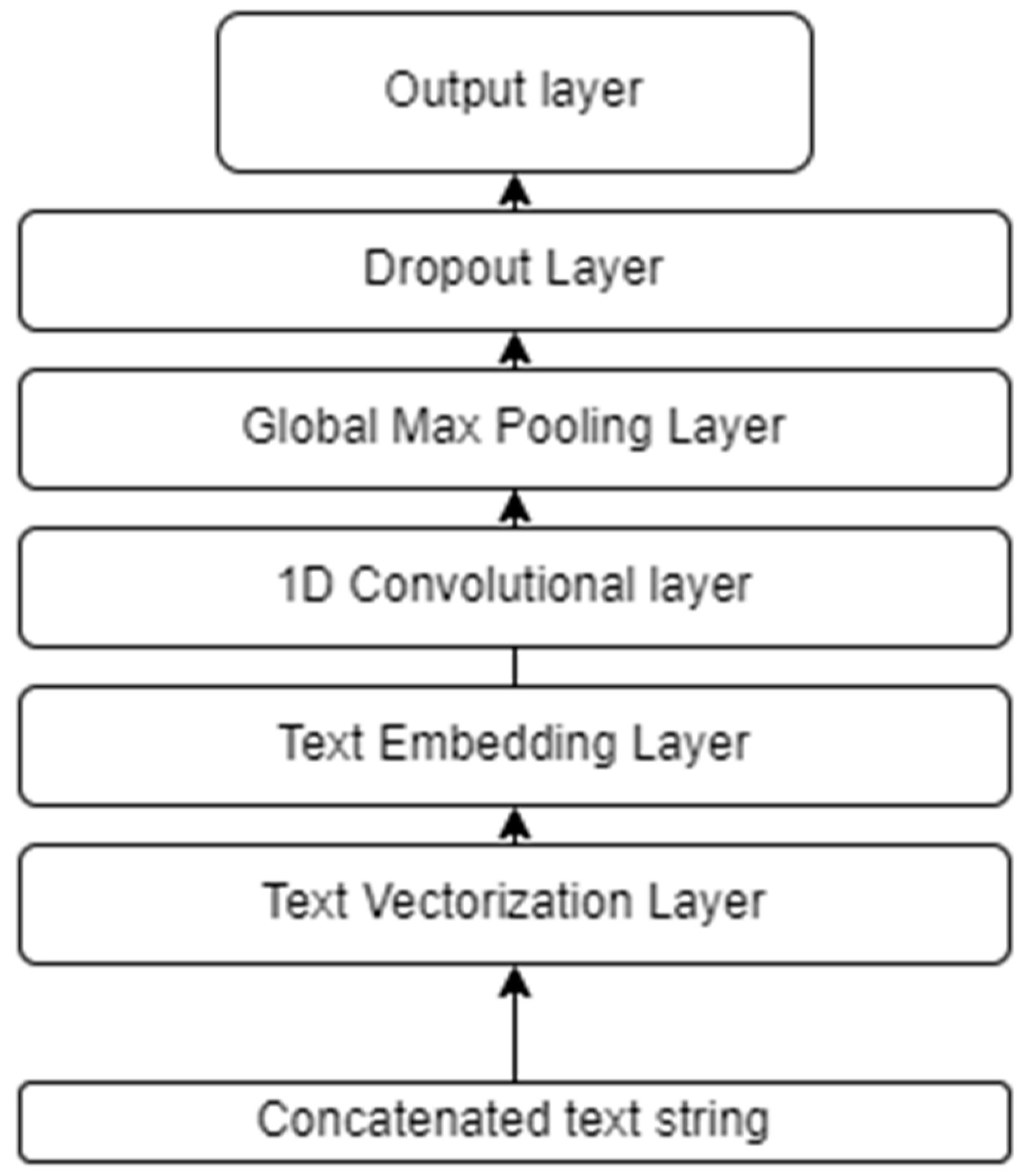
In this subsection, we propose our text classification model trained from scratch using the traditional approach. We propose a deep learning-based text classification model composed of the following layers.

Text Vectorization Layer

Text vectorization transforms a text string (of words) into a list of token indices based on a vocabulary. The vocabulary for the layer must be supplied on construction or learned from the training dataset. When the vocabulary is learned from the training data, the vectorization layer will analyze the dataset, determine the frequency of the values of the individual words, and create a vocabulary from them. The size of the vocabulary is usually capped; if there are more unique values in the input than the maximum vocabulary size, the most frequent words will be used to create the vocabulary.

Text Embedding Layer

Word embeddings are efficient, dense representations where similar words have a similar encoding. The embeddings are not specified manually; rather, they are trainable parameters optimized by the model during training in the same way a model learns weights for a dense layer. Word embedding vectors of different sizes or dimensions are common. A higher-dimensional embedding can capture more complex relationships between words but takes more data to learn.

Table 5. Examples of word embeddings.

Word	Embedding Vector
Sun	[1.2, −0.1, 4.3]
Earth	[2.1, 0.3, 0.1]
Water	[0.4, 2.5, −0.9]

illustrates how word embeddings might be for three different words. Each word is represented as a three-dimensional vector of numerical values. The embedding can be interpreted as a lookup table that maps from integer values (words) to dense vectors (word embeddings). The width (dimensionality) of the embedding is a parameter that can be adjusted, just like the size of a dense layer. The weights in the embedding layer are initialized randomly. During training, they are gradually adjusted through backpropagation. Once trained, the learned word embeddings will roughly encode similarities between words in the training dataset.

Convolutional Layer

A convolutional layer consists of multiple filters that are applied to the input data. Each filter is a vector of weights that is optimized based on the training data. This is carried out by calculating the element-wise product of the filter weights and the input data and taking the sum of these products, resulting in a measure of the correlation between the filter and the relevant part of the data. This is known as a convolved feature. After applying the filters to the input data, the resulting convolved features are passed through a non-linear, differentiable activation function, such as the rectified linear unit (ReLU) function. These filters can be seen as feature detectors; that is, they are used to detect specific patterns in the input data regardless of the location of the pattern in the input data structure. Using multiple filters in a convolutional layer allows one to identify several features simultaneously. Convolutional layers have significantly fewer trainable weights than fully connected layers, making it computationally feasible to stack multiple layers in a neural network.

Global Max Pooling Layer

Global max pooling is a pooling operation commonly used to reduce the spatial size of the feature maps by taking the maximum value of each feature map. This helps the network to focus on the most important features and reduce overfitting.

Dropout Layer

Dropout is a regularization technique that simply sets activation nodes to zero with a given probability during training (Srivastava et al. 2014). This prevents the network from adapting too much to the training data. During testing, the dropout layer scales the activations according to the dropout rate. We use dropout with a rate of 0.2 between the last two layers, but it can, in practice, be applied between any two layers.

Output Layer

The final layer has one output: the model prediction. The sigmoid activation function is applied to the output of the last hidden layer to ensure that the predictions are in the interval [0, 1], as follows:

$$Prediction\left(Z\right)=\frac{1}{1+e^{-Z}}$$

where Z refers to the output of the previous hidden layer.

Figure 1 illustrates the network architecture of the proposed model. In total, the model has 58,705 trainable weights. The network is trained to minimize the binary cross-entropy loss with respect to the weights using standard forward- and backpropagation.

3.2. A Deep Text Classification Model Based on Transfer Learning Using BERT

Our proposed deep text classification model (cf. Section 3.1) generates embeddings that are context-independent: i.e., there is just one representation (numeric vector) for each word. Different meanings of the word are combined into one single vector. In contrast, BERT (bidirectional encoder representations from transformers) (Devlin et al. 2018) and other large language models (LLMs) can create embeddings that allow us to have multiple vector representations for the same word, i.e., these embeddings are context-dependent. For example, the word “bank” can be used to describe a financial entity or land along a river (geography). While our proposed model in Section 3.1 will generate the same single vector for the word “bank”, the BERT model will generate at least two different vectors that will be used in two different contexts. One vector will be similar to certain words, such as money, cash, etc. The other vector would be similar to other vectors, such as beach, coast, etc.

In addition, NLP transformers, such as BERT, are trained on large corpora of text using self-supervised learning, and their resulting embeddings are more precise representations of words and context from natural language than if one were to train such models on a smaller dataset. These properties have propelled the use of transfer learning in NLP problems, where one typically finetunes LLM models with millions of pretrained weights on small datasets using supervised learning, resulting in state-of-the-art performance in several fields.

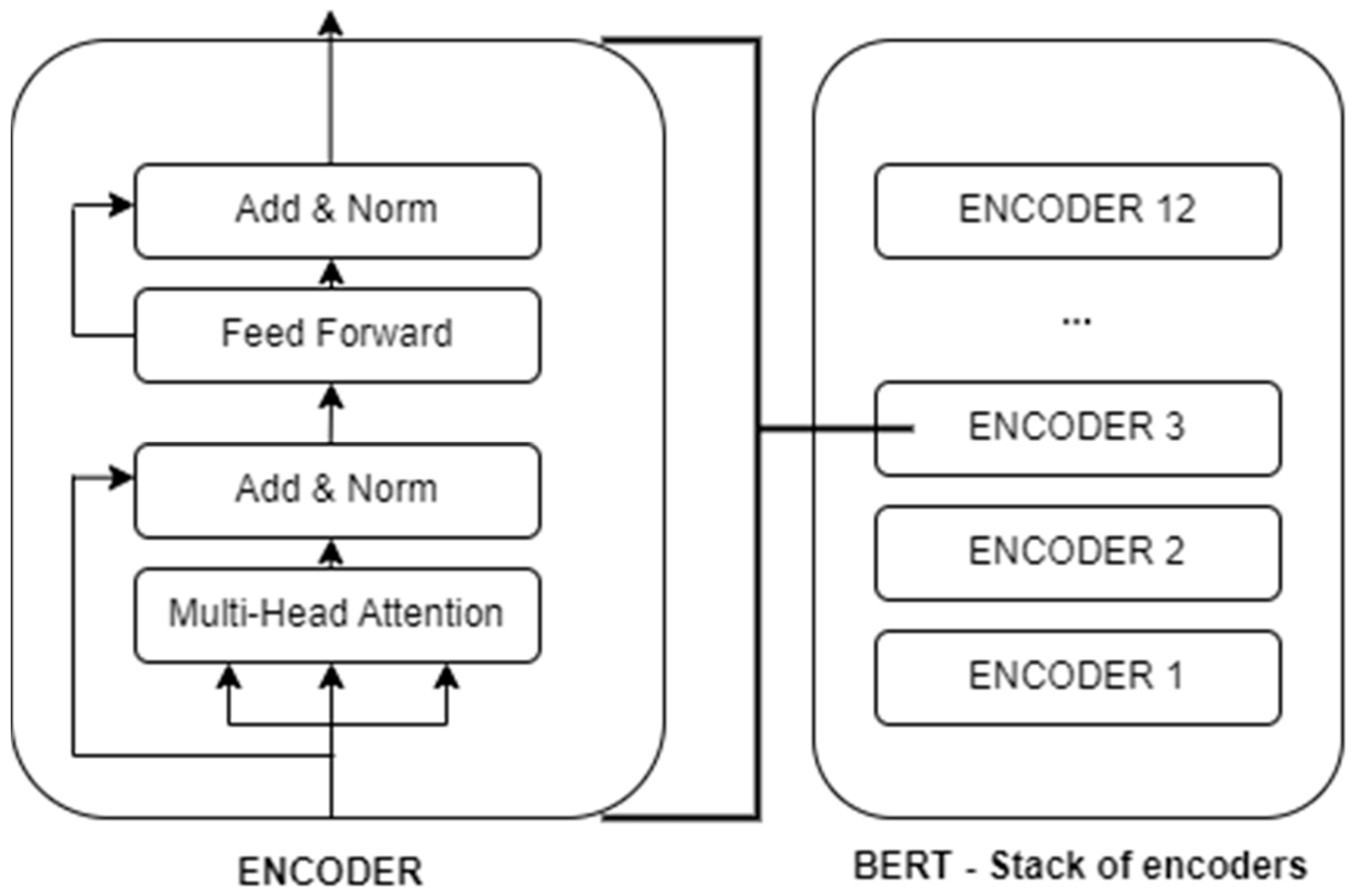
The network architecture of the model consists of a stack of transformer encoder layers through which an input text sequence is transformed into weighted vector representations (cf. Figure 2). The key difference from previous language models is the use of a bidirectional self-attention mechanism that enables the capturing of extensive contextual information. The transformer encoder blocks are composed of self-attention layers, which allow the model to attend to different parts of the input text at the same time, and feed-forward layers, which map the encoded input text to an output representation. These building blocks are what gives BERT its ability to capture the complex interactions between words in the input text and produce highly accurate predictions for a wide range of natural language processing tasks.

The output of the pre-trained BERT is a vector representation of size 1 × 768 for each input text string. The size of the vector depends on the network structure of BERT, which in the base model consists of 768 hidden layers (see Devlin et al. 2018). Thus, a text containing 1000 text strings is BERT-transformed into a matrix of 1000 × 768, representing the text and its contextual information.

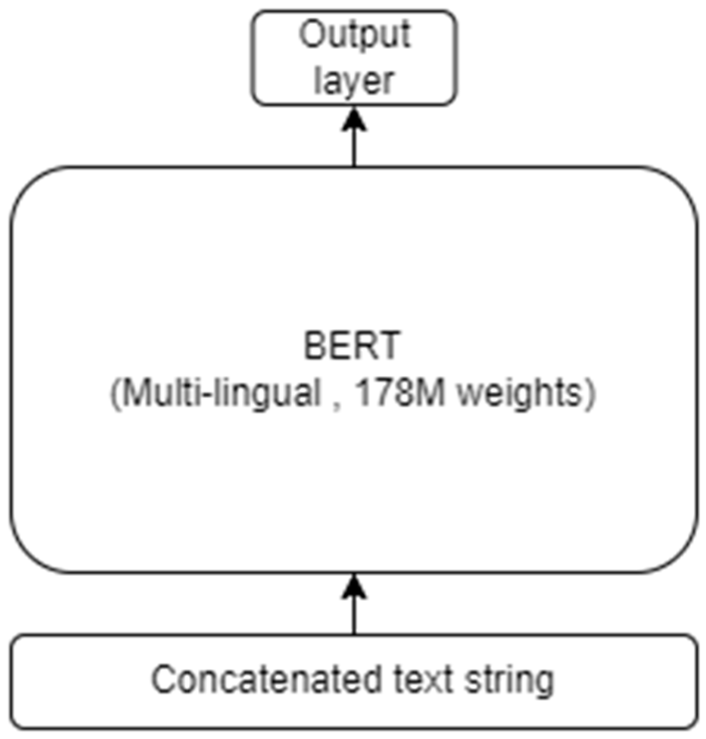
We propose a transfer learning based deep text classification model where we finetune a multilingual BERT to our training dataset. The network architecture is illustrated in Figure 3.

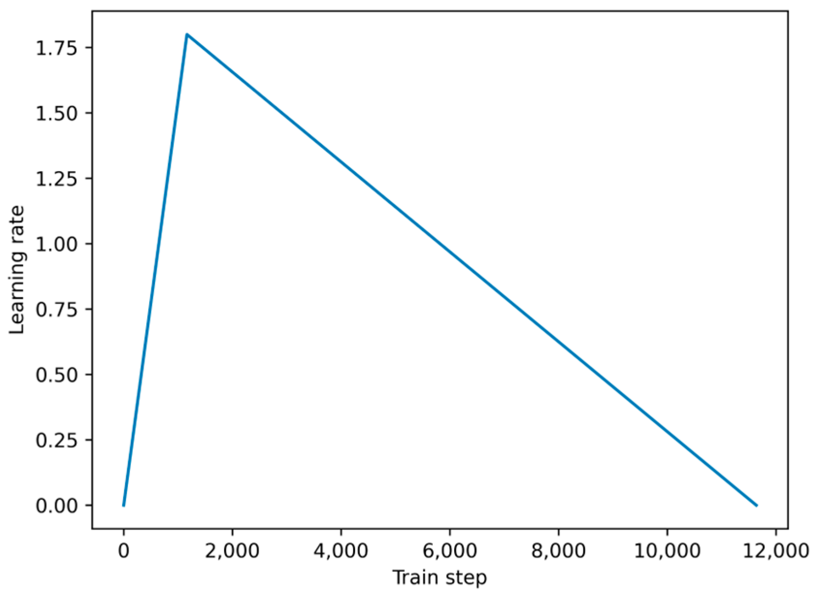
Our transfer learning model based on a multilingual BERT has 178 million weights. We finetune these using a warmup schedule during training, i.e., we increase the learning rate at the start of training before we decrease the learning rate towards zero at the end of training (cf. Figure 4). This approach helps the model converge faster and perform better on the finetuning task. Additionally, a warmup schedule can help prevent the model from becoming stuck in a suboptimal solution.

3.3. SHAP

SHAP (Shapley additive explanations), introduced by Lundberg and Lee (2017), is a framework for explaining individual predictions. The SHAP framework is based on Shapley values (Shapley 1952), originally used to calculate fair payouts in games, that is, payouts reflecting the players’ contribution to the total payout. Thus, SHAP values assume that the contribution (to the model prediction) of each possible coalition of features should be considered to determine the importance of a single feature.

In essence, Shapely values represent the average expected marginal contribution ${\varphi }_i$ of a feature i to the outcome (prediction) after all possible feature combinations have been checked. Here, we think of the text string as a set of players F and the words as embeddings (tokens). For token i, we compute the weighted marginal contribution on all subsets S in F that do not include i. The marginal contribution refers to the change in the output function v caused by the presence of i. Subsets that are close to the initial coalition or the empty set are given higher weights. Formally, the Shapley value of token i is as follows:

$${\varphi }_i\left(v,F\right)=\underset{Averaging}{\underbrace{\frac{1}{\left|F\right|}\sum _{S\subset F\left\{i\right\}}\underset{Combinatorialweights}{\underbrace{{\left(\genfrac{}{}{0pt}{}{\left|F\right|-1}{\left|S\right|}\right)}^{-1}}}\underset{Marginalcontribution}{\underbrace{\left[v\left(S\cup \left\{i\right\}\right)-v\left(S\right)\right]}}}}$$

According to Fadel (2022), Shapley values may be split into three components. The marginal contribution is how much the model changes when a new token $i$ is added. To obtain the overall effect of token $i$ on the final model, i.e., for our purpose the SHAP value of i for a bank customer, it is necessary to consider the marginal contribution of i in all the models where i is present. Given a set of features S, we denote $v\left(S\right)$ as the model trained with features $S$ present. $v\left(S\cup \left\{i\right\}\right)$ is the model trained with an extra token $i$. When these two models make different predictions, the quantity between square brackets is exactly how much they differ from each other. Combinatorial weight is the weight to give each of the different subsets of features with size $\left|S\right|$ (excluding the feature $i$). Finally, averaging will determine the average of all marginal contributions from all conceivable subset sizes ranging from $0$ to $\left|F\right|-1$. We must omit the one feature for which we wish to evalute the feature’s importance. The Shapley value is known to be the unique value that satisfies the following desirable properties:

-

Symmetry: If two tokens contribute equally to all possible coalitions, their contribution value is the same.

-

Efficiency: The sum of all Shapley values fully explains the gain or loss.

-

Dummy: A token that does not affect the result of the model has a contribution value of zero.

-

Additivity: When the output of a model is the additive result of two intermediate outputs, the new Shapley value is the sum of both intermediate Shapley values.

However, the estimation of the precise Shapley values faces some practical constraints due to the extremely high potential number of coalitions $\left(2^{\left|F\right|}\right)$. Calculation of the exact Shapley value is, therefore, computationally too costly. We must, therefore, resort to alternative, approximative methods, and they might affect whether some of these theoretical properties will hold (see, e.g., Aas et al. 2021).

The SHAP library offers a set of different approaches. For natural language processing, by default it computes the Owen value (Owen 1977), using the partition explainer. Owen values can be seen as the coalitional version of Shapley values, i.e., they consider that players may belong to groups. In our setting, this translates to token values being correlated. Although the main reason for SHAP’s partition explainer to use Owen values is to make computation more tractable, it is a nice side-effect that the use of Owen values alleviates the independence assumption problem by grouping highly correlated tokens together and thereby reducing the number of subsets on which marginal contributions need to be computed.

The main consequence when using Owen values as an approximation to Shapley values is that the symmetry property is breached. Contribution values depend on the initial partition and are, thus, now ambiguous.

3.4. Evaluation Metrics: AUC and Brier Score

To evaluate the performance of our credit risk models, two common metrics are typically used: the area under the receiver operating characteristic curve (AUC) and the Brier score.

The receiver operating characteristic (ROC) curve is a graphical representation of the balance between the true positive rate (sensitivity) and the false positive rate (1-specificity). It shows the performance of a classifier without considering the class distribution or the cost of misclassification. The area under the receiver operating characteristic curve (AUC) is a measure of a model’s discriminatory power across a range of cut-off points, and is calculated by determining the area under the ROC curve. It can be used to compare the performance of different classifiers and is useful in practical terms because banks may choose different cut-off points to manage risk tolerance. Additionally, the AUC metric is not sensitive to class imbalance, which is common in credit scoring.

The Brier score, developed by (Brier 1950), measures the accuracy of output predictions, as follows:

$$BS=\frac{1}{N}\sum _{i=1}^N{\left({y_i-PD}_i\right)}^2$$

In effect, it is the mean squared error but is used for binary prediction tasks. A predicted output (PD) that is closer to the true label (y) results in a smaller error. While a model should produce well-calibrated scores, it is not a requirement for a good classifier in practice, as the probability cut-off point can be adjusted accordingly. As such, the Brier score is considered a secondary metric to the AUC when evaluating model performance.

4. Results

4.1. Model Performance—Discriminatory Power (AUC) and Calibration (Brier Score)

We investigate the performance of two different credit scoring models based on the textual descriptions of customer transactions available from the open banking APIs: a model with weights trained from scratch and a model utilizing transfer learning using a multilingual BERT. The main results of our experiments can be found in

Table 6. Discriminatory power, AUC.

Model	Training Data	Validation Data	Test Data
Deep text classification model (trained from scratch)	85.6%	84.7%	90.9%
BERT transfer learning model	81.5%	79.2%	82.5%

and

Table 7. Brier score.

Model	Training Data	Validation Data	Test Data
Deep text classification model (trained from scratch)	0.129	0.061	0.015
BERT transfer learning model	0.154	0.067	0.023

.

The results in Table 6 show the models’ discriminatory power, or ability to distinguish between good and bad credit risks, as measured by the area under the curve (AUC) of the receiver operating characteristic (ROC) curve. The AUC measures the model’s ability to correctly classify good and bad credit risks, with a higher AUC indicating better performance. The results in Table 6 show that the deep text classification model has a higher AUC than the BERT transfer learning model on all three datasets: training, validation, and test. The results in Table 7 show the Brier score, which measures the accuracy of probabilistic predictions. It is calculated as the mean squared difference between the predicted probability and the actual outcome. A lower Brier score indicates better performance. The results in Table 7 show that the deep text classification model has a lower Brier score than the BERT transfer learning model on all three datasets: training, validation, and test.

Overall, these results suggest that the deep text classification model performs better than the BERT transfer learning model in terms of both discriminatory power and accuracy of probabilistic predictions.

4.2. Model and Prediction Explainability (SHAP)

We apply SHAP values to provide explanations of the workings of the best-performing deep learning model (trained from scratch). Since banks are primarily interested in explaining potential loan application rejections and the fact that calculating SHAP values are computationally expensive, we focus on high-risk cases in our analysis. Furthermore, by calculating SHAP values based on high-risk cases, we can identify which features are most important in driving the model’s prediction of high-risk. This approach can help us understand the factors most relevant to the model’s decision.

In our analysis, we set the PD threshold to 25%. This threshold is determined on a discretionary basis to make it possible to carry out the SHAP calculations within a reasonable time, given the computational resources available for this study. The relatively high threshold must be seen in relation to the fact that the model is not properly calibrated to the large test sample. The SHAP values in the following analysis are, thus, based on the 1,166 cases from the large test sample where the model predicts the default probability to be greater than 25%.

In the following, we split our analysis into two parts, namely a global explanation of the model (“what drives the model”) and local explanations (“explaining factual model predictions”).

4.2.1. Global Explainability

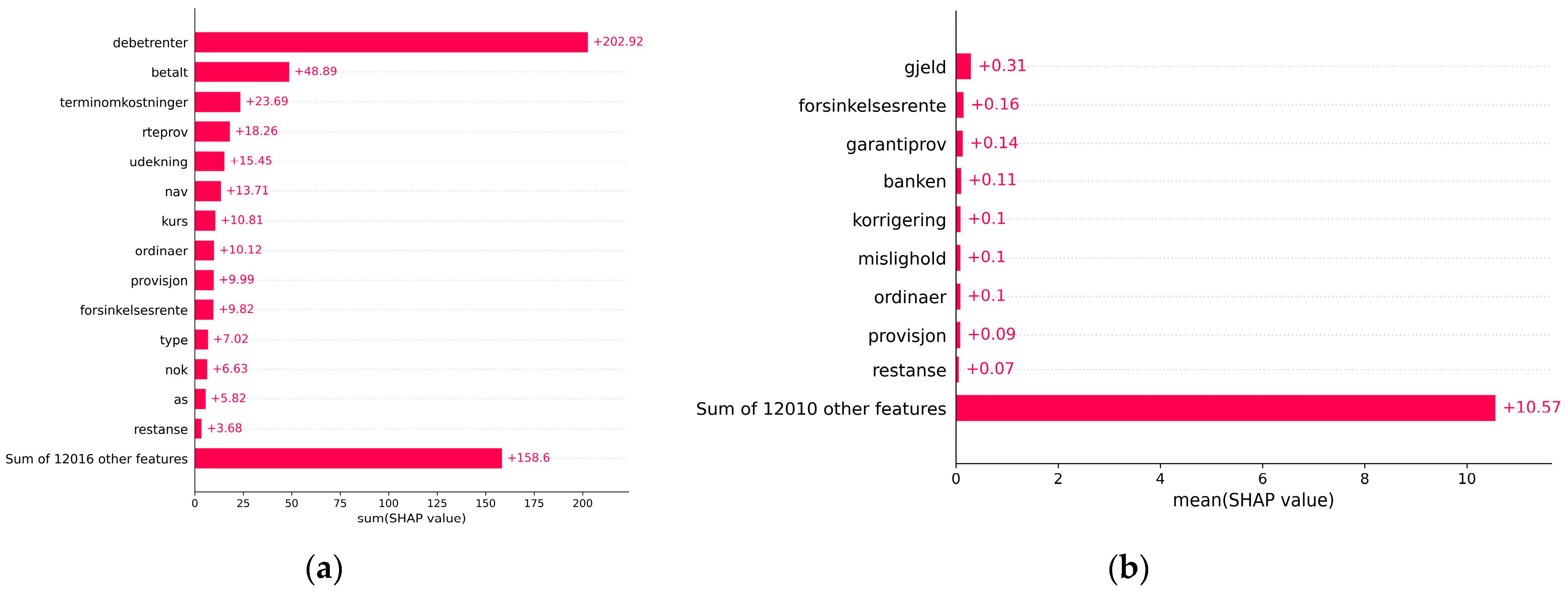
When evaluating the global explainability of our deep learning model, we focus on how much each word contributes, aggregated over all customers’ PDs. Figure 5a shows the most contributing words based on the sum of SHAP values, while Figure 5b shows the most contributing words based on the mean of SHAP values across our 1166 high-risk cases. The words in Figure 5a,b are ranked by importance, and some words are excluded for privacy reasons. The excluded words are not considered important when interpreting the model or its predictions.

Both figures are relevant when interpreting the model. For example, while “debetrenter” (English: “debit interest”) is by far the most contributing word to PDs for high-risk cases in sum (cf. Figure 5a), it is not among the most contributing words when considering the mean contribution (cf. Figure 5b). “Debetrenter” is paid if the current account balance is below zero and might indicate financial hardship in some cases, e.g., for long periods of account overdrafts, while short and infrequent cases of overdrafts might be of less concern. Other words from Figure 5a that might be relevant in identifying high-risk cases are “udekning” (English: payment without sufficient funds), and “nav” (English: a government agency in Norway that is responsible for providing financial assistance and support to individuals and families who are in need). The words “gjeld” (English: debt) and “mislighold” (English: default) from Figure 5b also seem relevant in this regard.

Words that are present in both Figure 5a,b are common among high-risk cases and have, at the same time, a high contribution on average to these cases’ PDs, and are, therefore, considered highly relevant when identifying high-risk cases. Examples are “forsinkelsesrente” (English: “late payment interest” or “late fee”) and “restanse” (English: “arrears”).

4.2.2. Local Explainability

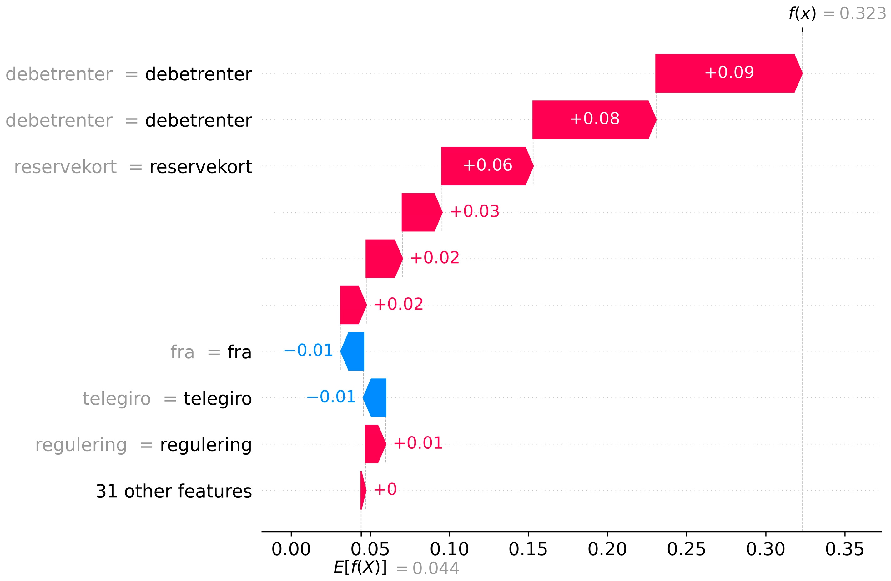
SHAP can provide detailed and intuitive explanations for individual predictions through waterfall plots. These plots illustrate the contribution of each word to the default prediction, with red and blue bars representing positive and negative contributions, respectively. The words are ranked by importance, and the actual words are displayed on the left side. In the following waterfall plots, the prediction by the deep text classification model (trained from scratch) is displayed as f(x), and the positive bias or intercept from the model is shown below the plot as E[f(x)], both measured in probability (of default).

We use waterfall plots to examine three selected cases and try to interpret why the model has assigned relatively high PD to these cases.

Figure 6 shows which words that contribute the most to the PD of our selected case number 1. In this case, the text string contains 40 words from transactions completed during the past 90 days. The figure shows that the words “debetrenter” (+8 pp. and +9 pp.) and “reservekort” (+6 pp.) contribute the most to the customer’s high PD (32.3%), while the words “fra” (English: “from”) and “telegiro” reduces the PD by 1 pp. each. Three highly contributing words are anonymized for privacy reasons.

The two instances of “debetrenter” are connected to two periods of overdrafts, where the first is an overdraft of a “reservekort” (English: a type of credit card), while the second is a period of overdraft of the current account. The model identifies this as high-risk behavior. We observe that this is also the case for other high-risk cases with “debetrenter” in which the number of words (and transactions) is relatively low. Furthermore, we observe that the inflow of funds (deposits or payments) to this account (represented by the words “fra” and “telegiro”) reduces the PD somewhat.

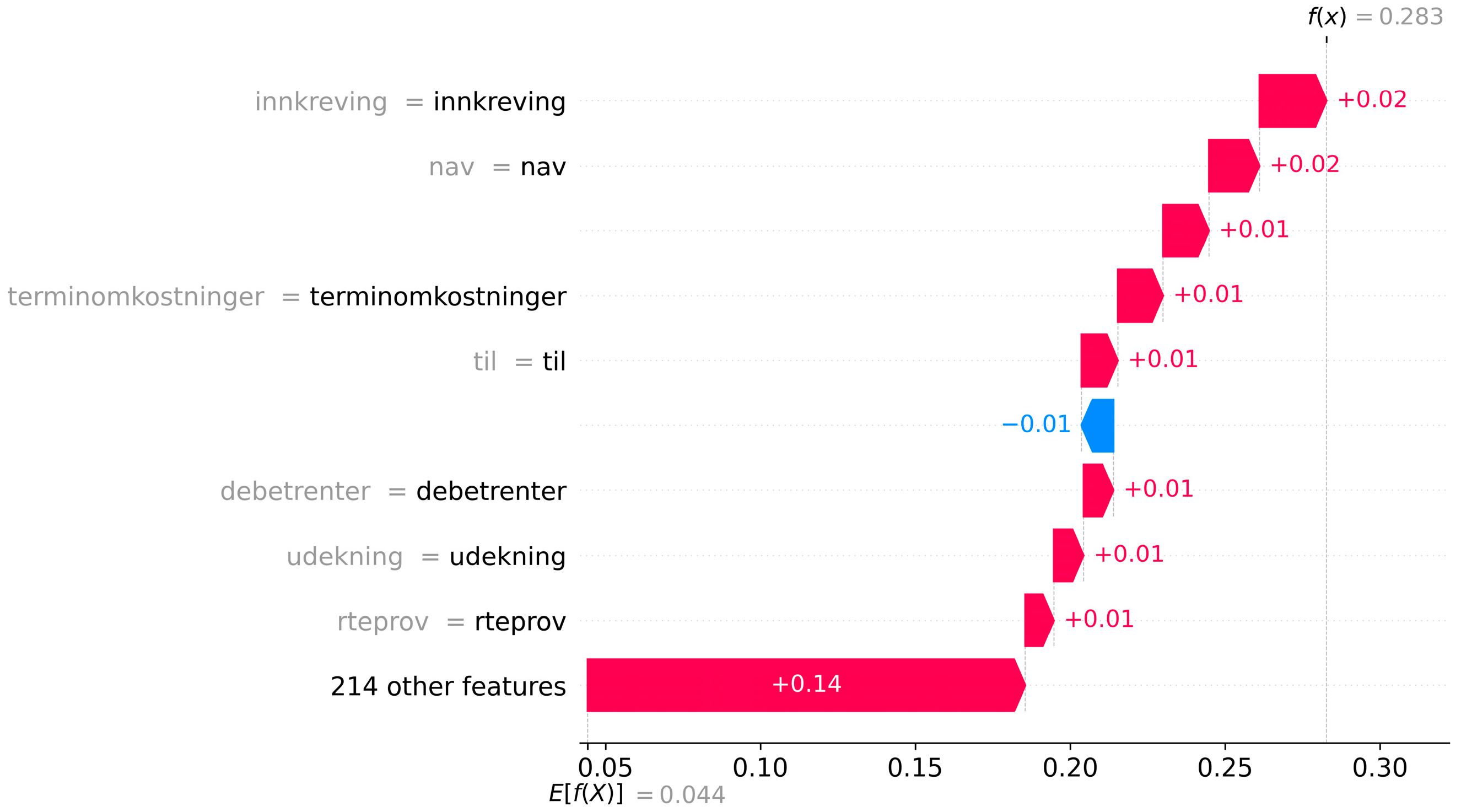
In case 2, cf. Figure 7, the text string contains over 200 words describing the transactions completed by the customer during the past 90 days. In contrast to case 1, where a few words explained most of the high PD, the model emphasizes several words when assigning the high PD of 28.3% to case 2.

The most contributing words are “innkreving” (English: collection) and “nav” (+2 pp). In this case, this indicates that the customer is subject to collection measures by NAV, a Norwegian government organization. Furthermore, the model emphasizes the words “debetrenter” and “udekning”, which indicates a period of overdraft of the current account and payment without sufficient funds. The abovementioned words can be interpreted as high-risk behavior by the customer. Other words, such as “terminkostnader”, “rteprov” and “til,” are also emphasized by the model. Finally, we notice that the remaining 214 words contribute +14 pp. in sum when calculating the PD.

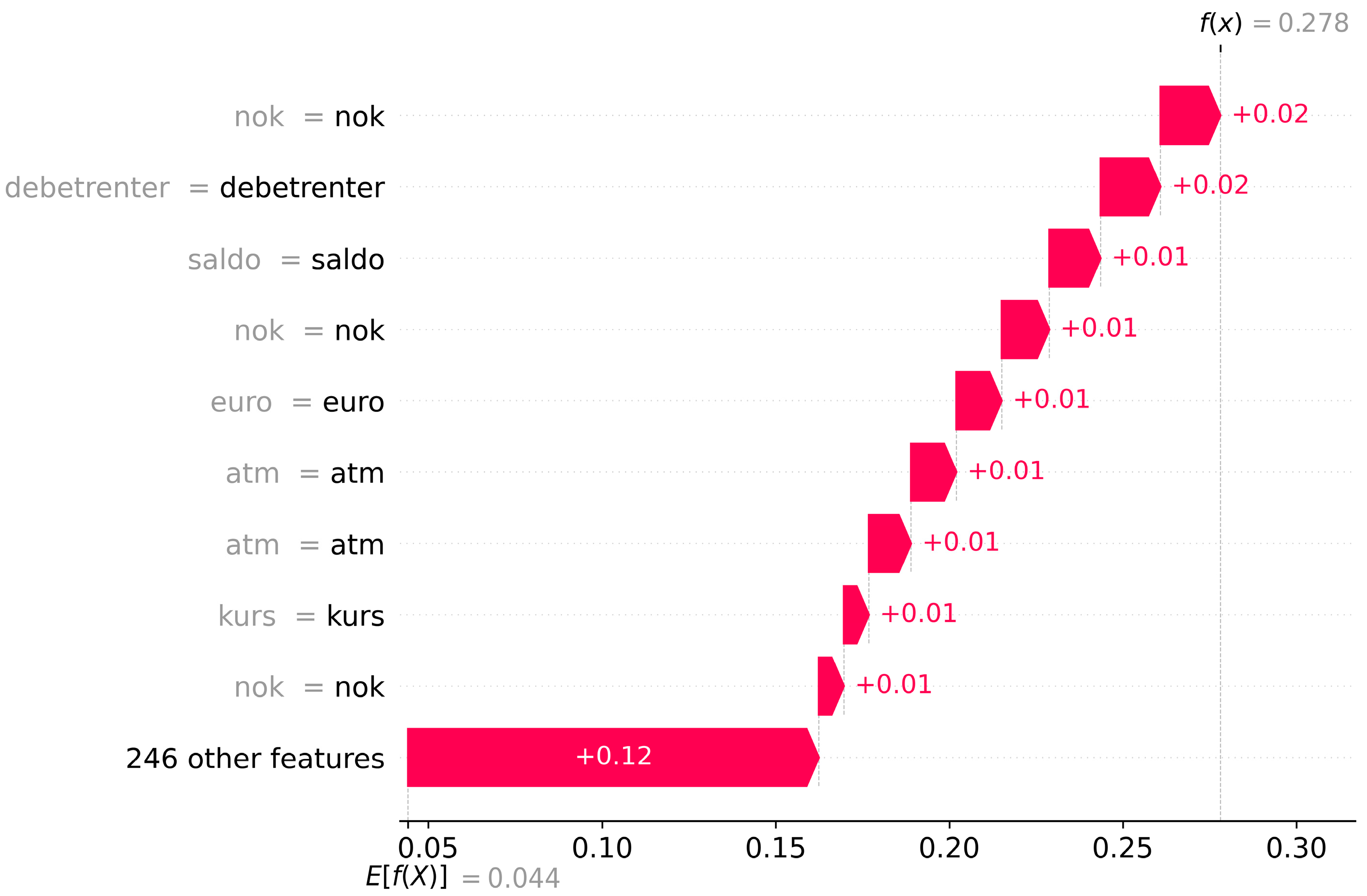
Figure 8 shows the words emphasized by the model for case 3. Here the customer is assigned a PD of 27.8%, whereas “debetrenter” and several instances of “nok” (the currency of Norway), “atm”, “saldo” (English: account balance), “euro”, and “kurs” (English: exchange rate) are the most contributing words. The customer is registered with an overdraft of the current account and, during the same period, has several cash withdrawals from ATMs abroad. The model interprets this as high-risk behavior by the customer. The remaining 246 words from transactions completed during the last 90 days contribute 12 pp in sum when calculating the PD.

5. Discussion

In our experiments, we found that the deep learning model trained from scratch outperformed the model using transfer learning with a multilingual BERT in terms of both discriminatory power and accuracy of probabilistic predictions. This can be attributed to the fact that the deep text classification model was trained from scratch using the training data, while the BERT transfer learning model utilized pre-trained multilingual BERT weights trained on more unrelated text data and was only finetuned using the training data.

This indicates that while the text strings from transaction data may contain words seen in the training data for the multilingual BERT, they do not contain natural sentences, and the context of the words is, therefore, less important. The main strength of transformer models, such as BERT, is the ability to account for the context of words in a sentence or text, and we interpret the inferior performance of the BERT transfer model as an indication that context is less important when the model input is concatenated text strings from bank transaction data.

These results align with the findings of Kriebel and Stitz (2022), who attributed the superior performance of simpler models trained from scratch to the shorter textual strings used in their study. They posited that the limited context within these short strings may reduce the effectiveness of finetuned BERT models, which are designed to excel at capturing contextual information in longer, more complex sentences. Conversely, Stevenson et al. (2021) employed a finetuned BERT model on longer text strings containing natural language (textual credit assessments by credit officers) and observed that their BERT model outperformed other machine learning-based models trained from scratch.

Our study contributes to this ongoing debate by demonstrating that, for the specific task of credit scoring modeling based on short transaction descriptions, a deep learning model trained from scratch can indeed outperform a BERT transfer learning model. This discrepancy suggests that the applicability of transfer learning models, such as BERT, may vary depending on the nature and length of the textual data used, and emphasizes the need for further investigation into the performance of these models across different data types and problem domains.

Furthermore, the superior results of the deep text classification model trained from scratch are encouraging for incumbent banks, since this clearly indicates that text strings from bank transaction data are highly predictive of future defaults, even when restricted to the past 90 days before the score date. This result shows that such text strings available through open banking API might be highly valuable for incumbent banks when developing application credit scoring models for new, potential customers. In addition, while the BERT transfer learning model performs worse than the model trained from scratch, the BERT model performance can be considered satisfactory. Therefore, such models might be valuable for FinTech companies and other financial intermediates who do not have access to large amounts of historical transactions when developing new products and services based on the data available through the open banking APIs.

Our findings align with the results of Kvamme et al. (2018), and Hjelkrem et al. (2022a, 2022b). These studies also discovered that information available through open banking APIs, specifically daily balances and transaction amounts, are highly predictive of future defaults among bank customers. Kvamme et al. (2018) demonstrated the predictive power of daily balances by employing various machine learning techniques on a dataset of bank customers. In contrast, Hjelkrem et al. (2022a, 2022b) focused on transaction amounts, with the former extending Kvamme et al.’s work by incorporating more detailed data and advanced algorithms, and the latter comparing the performance of such deep learning models with conventional credit scoring models based on aggregated, tabular datasets, revealing how transaction amounts can be used to increase model performance when recruiting new customers.

While our study focuses on text strings from transaction data, the results of Kvamme et al. (2018) and Hjelkrem et al. (2022a, 2022b) indicate that other forms of data available through open banking APIs can also be used to predict future defaults. This suggests that a combination of transaction descriptions, daily balances, and transaction amounts might lead to even more powerful credit scoring models. It is worth noting that these studies, together with our findings, underscore the value of open banking APIs for credit scoring purposes. By incorporating various data types and leveraging machine learning techniques, incumbent banks, FinTech companies, and other financial intermediates can develop more accurate and comprehensive credit scoring models.

The SHAP analysis in our study advances the understanding of global and local explanations for deep learning model predictions in the context of credit scoring. Our global explainability results revealed that specific words, such as “debetrenter” (English: debit interest), “udekning” (English: payment without sufficient funds), “for-sinkelsesrenter” (English: late payment interest), “restanse” (English: arrears), and “mislighold” (English: default), played a significant role in the model’s prediction of high risk. This finding is consistent with the credit risk modeling literature, which often incorporates variables based on aggregates of such behavioral information in traditional credit scoring models. However, our study extends the existing literature by applying SHAP analysis to deep learning models based on raw, unaggregated transaction data, providing valuable insights into the underlying behavior and the factors driving its predictions.

Our contributions can be further contextualized by comparing our results with Melsom et al. (2022), who demonstrated that SHAP can be used to explain predictions from “shallow” machine learning models, such as LightGBM and logistic regression, trained on conventional credit scoring datasets consisting of aggregated features handmade by experts. While both our study and Melsom et al. (2022) leverage SHAP analysis to provide explanations for model predictions, the key difference lies in the type of data and models used. Melsom et al. (2022) focused on “shallow” machine learning models trained on conventional credit scoring datasets with aggregated features created by experts. In contrast, our study applies SHAP analysis to deep learning models trained on raw, unaggregated transaction data.

This distinction highlights the versatility of SHAP analysis in providing interpretable insights for various models and data types. Our study contributes to the literature by demonstrating that SHAP analysis can be effectively applied to deep learning models based on raw transaction data, emphasizing its value in extracting meaningful explanations for complex models in the field of credit scoring.

6. Conclusions and Implications

Overall, these results suggest that the deep learning model trained from scratch is a better choice for credit scoring based on textual descriptions of customer transactions available through open banking APIs. Furthermore, we conclude that SHAP can be a valuable tool for providing both global and local explanations of the model’s predictions and can be used to explain loan application rejections based on deep learning models.

The implications of this study are significant for incumbent banks in several ways. First, the study shows that textual descriptions from open banking data can be a valuable data source for banks when developing credit scoring models for new, potential customers. By including this type of data, banks can improve the performance of their credit scoring models and better predict future defaults when recruiting new customers. This can ultimately lead to reduced credit losses and improved profitability for incumbent banks.

Second, the study highlights the usefulness of SHAP as a tool for explaining high-PD predictions. This can help banks comply with the “rights to explanation” requirements in GDPR, which stipulate that individuals have the right to know the reasoning behind decisions that are made about them using automated systems. By providing explanations for high-PD predictions (i.e., loan rejections), banks can improve transparency and trust with their customers, potentially gaining a competitive advantage in the market.

Third, it is worth noting that the explainability and interpretability of credit scoring models are crucial requirements for regulatory approval. As such, incumbent banks should consider incorporating explainability tools, such as SHAP, when implementing machine learning-based credit scoring models, enabling them to comply with regulatory requirements.

Limitations and Further Research

This study is based solely on data from a Norwegian bank’s current customers. The results in this study are, therefore, not necessarily fully transferable to the assessment of actual applications from new customers, and future research should focus on developing credit scoring models on data from actual application cases where open banking data are obtained as a part of the application assessment process. Furthermore, since the analysis in this study is based on data from a single Norwegian bank, the results may not necessarily be transferable to other banks or countries. Additionally, while the Shapley value approach used by SHAP provides an interesting attempt to explain the outcome of the model, approximation techniques must be used, since the estimation of the precise Shapley values is challenging due to the extremely high potential number of feature combinations. This might affect the validity of the results.

Future research could, therefore, focus on expanding the scope of datasets used to include a wider range of institutions and countries and more robust approximation techniques for SHAP. In addition, further research could focus on identifying ways to improve the performance of deep learning-based credit risk models using transfer learning techniques and investigating other methods and tools for explaining predictions from deep learning-based credit risk models, such as causal inference models.