
Modeling the Characteristics of Unhealthy Air Pollution Events: A Copula Approach

Abstract
:1. Introduction
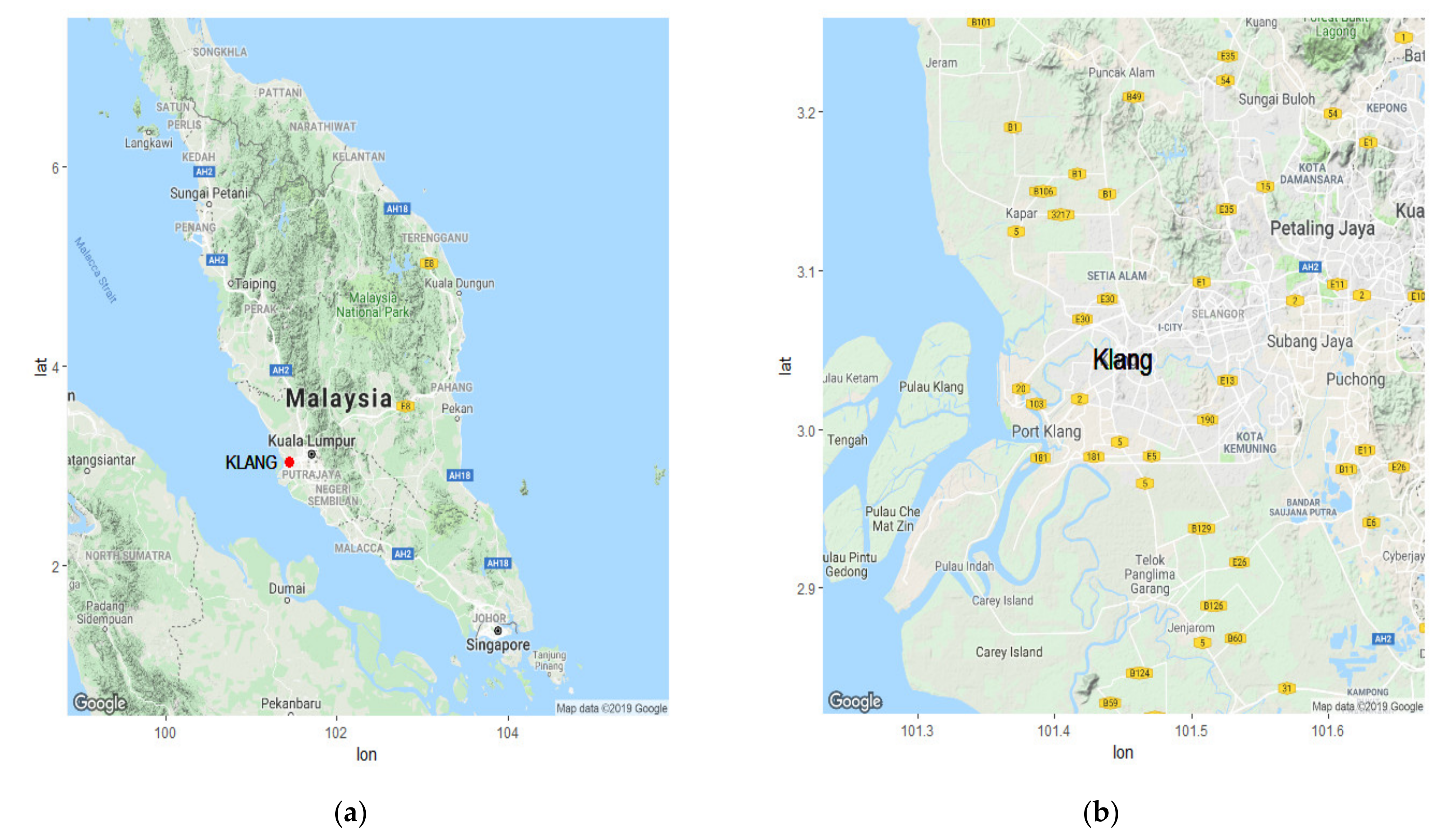
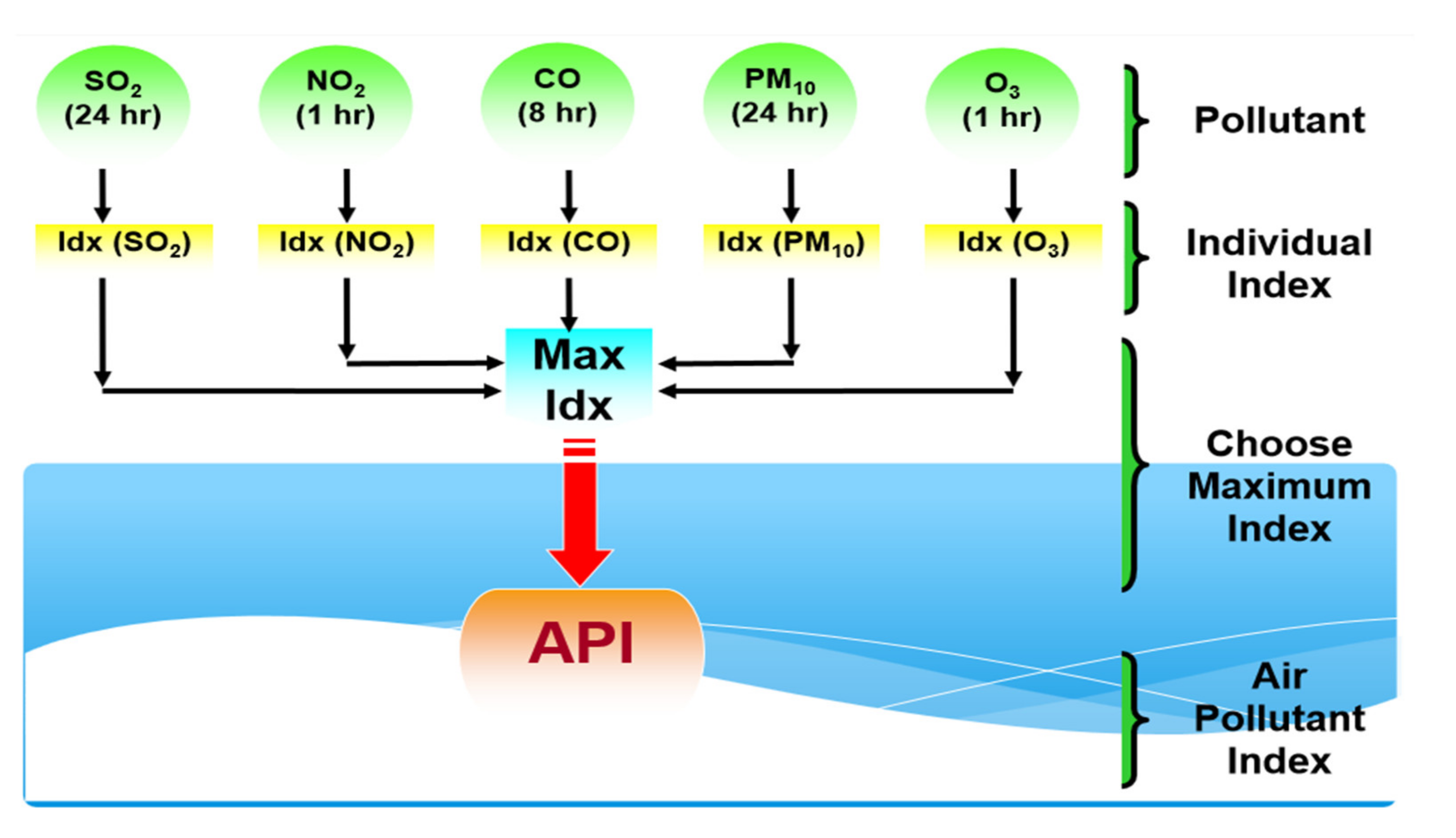
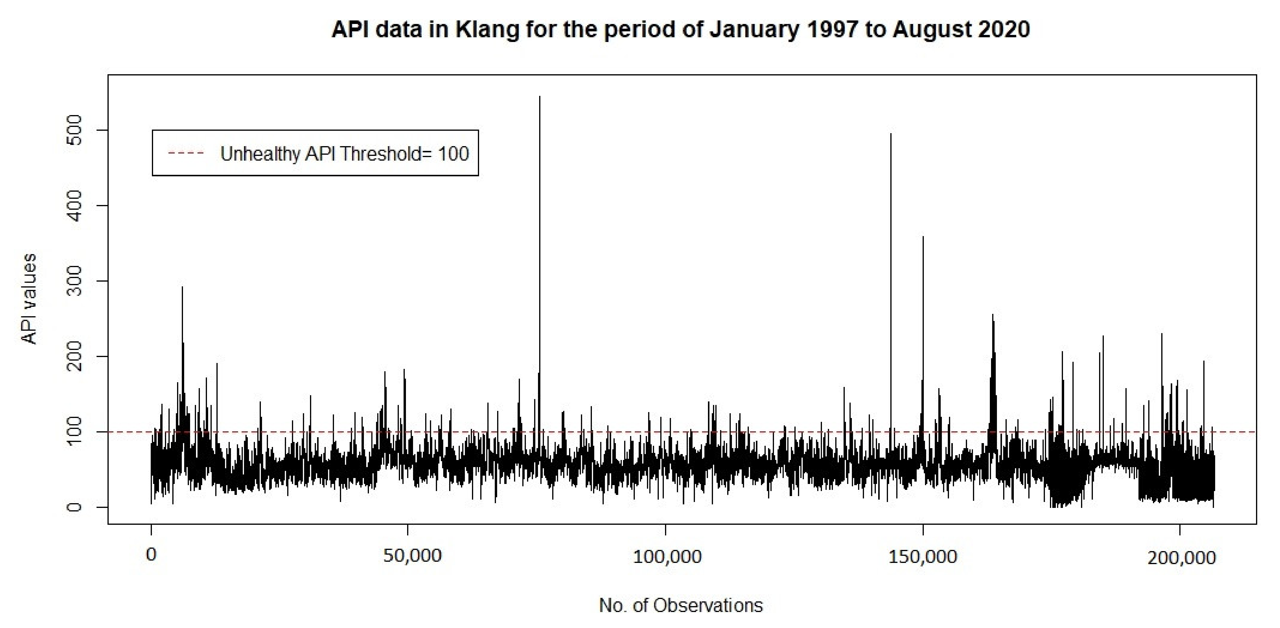
2. Study Area and Data
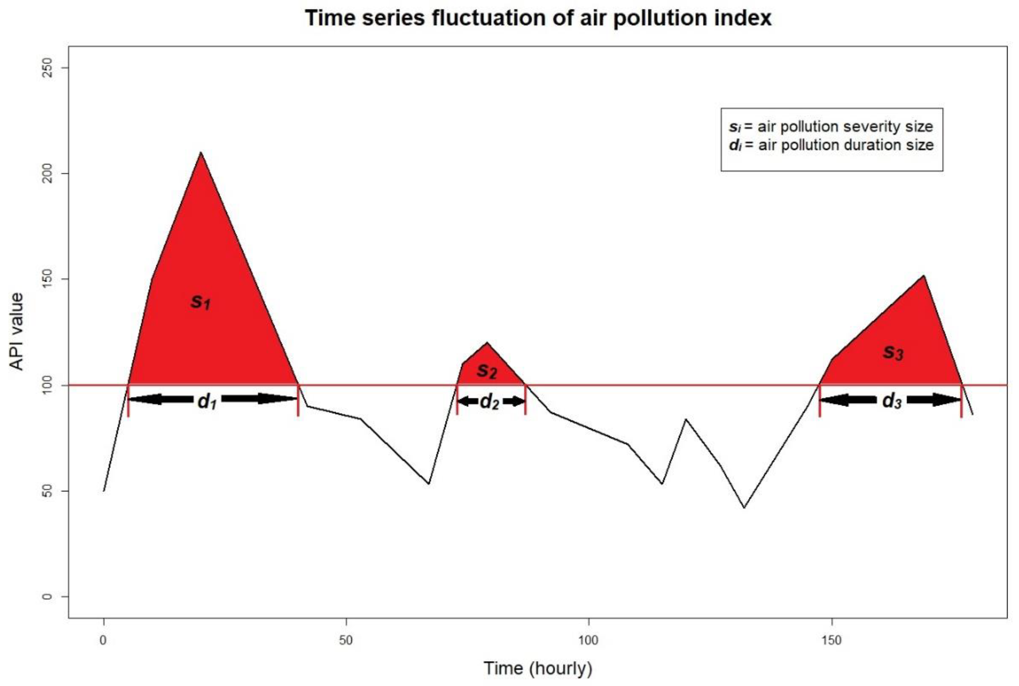
3. Copula Description of Air Pollution Characteristics
4. Copula Models
4.1. Clayton Copula
4.2. Ali–Mikhail–Haq (AMH) Copula
4.3. Frank Copula
4.4. Plackett Copula
4.5. Gumbel–Hougaard (GH) Copula
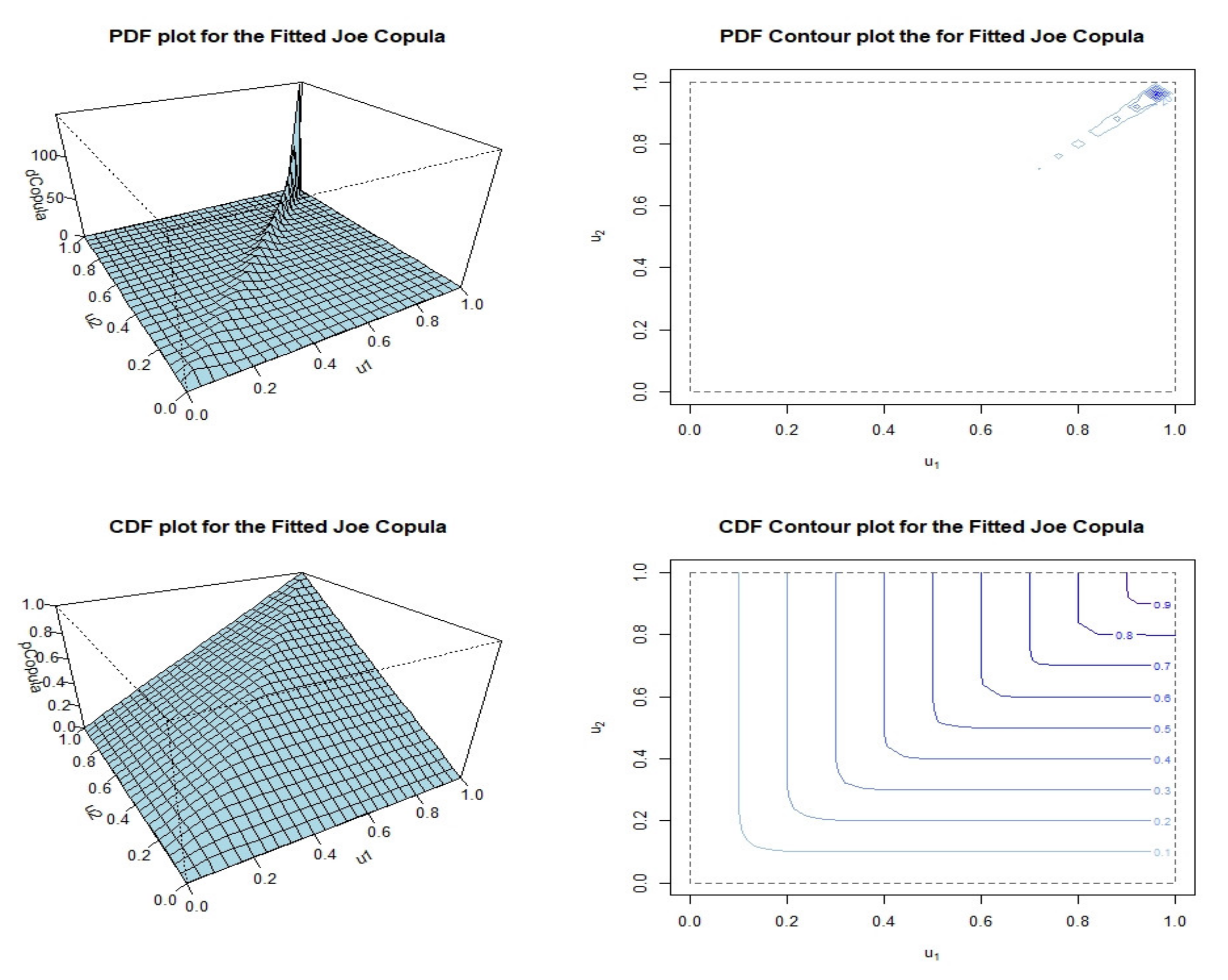
4.6. Joe Copula
5. Parameter Estimation and Model Selection
5.1. Pseudo Maximum Likelihood Estimation (Pseudo-MLE)
5.2. Cross-Validation Copula Information Criterion (cvCIC)
6. Results and Discussion
7. Conclusions
Funding
Institutional Review Board Statement
Informed Consent Statement
Data Availability Statement
Acknowledgments
Conflicts of Interest
References
- Murena, F. Measuring air quality over large urban areas: Development and application of an air pollution index at the urban area of Naples. Atmos. Environ. 2004, 38, 6195–6202. [Google Scholar] [CrossRef]
- Masseran, N. Modeling fluctuation of PM10 data with existence of volatility effect. Environ. Eng. Sci. 2017, 34, 816–827. [Google Scholar] [CrossRef]
- Masseran, N. Power-law behaviors of the duration size of unhealthy air pollution events. Stoch. Environ. Res. Risk Assess. 2021, 35, 1499–1508. [Google Scholar] [CrossRef]
- Genest, C.; Quessy, J.-F.; Rémillard, B. Goodness-of-fit procedures for copula models based on the probability integral trans-formation. Scand. J. Stat. 2006, 32, 337–366. [Google Scholar] [CrossRef]
- Huard, D.; Évin, G.; Favre, A.-C. Bayesian copulas selection. Comput. Stat. Data Anal. 2006, 51, 809–822. [Google Scholar] [CrossRef]
- Marcotte, D.; Henry, E. Automatic joint set clustering using a mixture of bivariate normal distributions. Int. J. Rock Mech. Min. Sci. 2002, 39, 323–334. [Google Scholar] [CrossRef]
- Lai, C.D.; Balakrishnan, N. Continuous Bivariate Distributions; Springer: Berlin/Heidelberg, Germany, 2009. [Google Scholar] [CrossRef]
- Tran, K.P.; Castagliola, P.; Celano, G. Monitoring the ratio of population means of a bivariate normal distribution using CUSUM type control charts. Stat. Pap. 2016, 59, 387–413. [Google Scholar] [CrossRef]
- Choi, J.-E.; Shin, D.W. Three regime bivariate normal distribution: A new estimation method for co-value-at-risk, CoVaR. Eur. J. Financ. 2019, 25, 1817–1833. [Google Scholar] [CrossRef]
- Yue, S. The bivariate lognormal distribution to model a multivariate flood episode. Hydrol. Process. 2000, 14, 2575–2588. [Google Scholar] [CrossRef]
- Pundir, S.; Amala, R. Detecting diagnostic accuracy of two biomarkers through a bivariate log-normal ROC curve. J. Appl. Stat. 2015, 42, 2671–2685. [Google Scholar] [CrossRef]
- Gumbel, E.J. Bivariate logistic distributions. J. Am. Stat. Assoc. 1961, 56, 335–349. [Google Scholar] [CrossRef]
- Yue, S. The Gumbel logistic model for representing a multivariate storm event. Adv. Water Resour. 2000, 24, 179–185. [Google Scholar] [CrossRef]
- Yue, S.; Ouarda, T.; Bobée, B.; Legendre, P.; Bruneau, P. The gumbel mixed model for flood frequency analysis. J. Hydrol. 1999, 226, 88–100. [Google Scholar] [CrossRef]
- Yue, S. A bivariate extreme value distribution applied to flood frequency analysis. Hydrol. Res. 2001, 32, 49–64. [Google Scholar] [CrossRef]
- Marshall, A.W.; Ingram, O. A multivariate exponential distribution. J. Am. Stat. Assoc. 1967, 62, 30–44. [Google Scholar] [CrossRef]
- Bacchi, B.; Becciu, G.; Kottegoda, N. Bivariate exponential model applied to intensities and durations of extreme rainfall. J. Hydrol. 1994, 155, 225–236. [Google Scholar] [CrossRef]
- Won, J.; Choi, J.; Lee, O.; Park, M.J.; Kim, S. Two ways to quantify Korean drought frequency: Partial duration series and bivariate exponential distribution, and application to climate change. Atmosphere 2020, 11, 476. [Google Scholar] [CrossRef]
- Royen, T. Expansions for the multivariate chi-square distribution. J. Multivar. Anal. 1991, 38, 213–232. [Google Scholar] [CrossRef] [Green Version]
- Izawa, T. Two or multi-dimensional gamma-type distribution and its application to rainfall data. Pap. Meteorol. Geophys. 1965, 15, 167–200. [Google Scholar] [CrossRef] [Green Version]
- Moran, P.A.P. Statistical inference with bivariate gamma distribution. Biometrika 1969, 54, 385–394. [Google Scholar] [CrossRef]
- Schmeiser, B.W.; Lal, R. Bivariate gamma random vectors. Oper. Res. 1982, 30, 355–374. [Google Scholar] [CrossRef]
- Loaciga, H.A.; Leipnik, R.B. Correlated gamma variables in the analysis of microbial densities in water. Adv. Water Resour. 2005, 28, 329–335. [Google Scholar] [CrossRef]
- Yue, S.; Ouarda, T.; Bobée, B. A review of bivariate gamma distributions for hydrological application. J. Hydrol. 2001, 246, 1–18. [Google Scholar] [CrossRef]
- Nadarajah, S. A bivariate gamma model for drought. Water Resour. Res. 2007, 43, W08501. [Google Scholar] [CrossRef] [Green Version]
- Antão, E.M.; Soares, C.G. Approximation of the joint probability density of wave steepness and height with a bivariate gam-ma distribution. Ocean. Eng. 2016, 126, 402–410. [Google Scholar] [CrossRef]
- Lambert, P.; Vandenhende, F. A copula-based model for multivariate non-normal longitudinal data: Analysis of a dose titra-tion safety study on a new antidepressant. Stat. Med. 2002, 21, 3197–3217. [Google Scholar] [CrossRef] [PubMed] [Green Version]
- Joe, H. Dependence Modeling with Copulas; Chapman and Hall/CRC: New York, NY, USA, 2014. [Google Scholar] [CrossRef]
- Hofert, M.; Kojadinovic, I.; Mächler, M.; Yan, J. Elements of Copula Modeling with R; Springer: Berlin/Heidelberg, Germany, 2018. [Google Scholar] [CrossRef]
- Kojadinovic, I.; Yan, J. Modeling multivariate distributions with continuous margins using the copula R package. J. Stat. Softw. 2010, 34, 17192. [Google Scholar] [CrossRef] [Green Version]
- Zhang, L.; Singh, V.P. Copulas and Their Applications in Water Resources Engineering; Cambridge University Press: Cambridge, UK, 2019. [Google Scholar] [CrossRef] [Green Version]
- Sak, H.; Yang, G.; Li, B.; Li, W. A copula-based model for air pollution portfolio risk and its efficient simulation. Stoch. Environ. Res. Risk Assess. 2017, 31, 2607–2616. [Google Scholar] [CrossRef]
- Chan, R.K.S.; So, M.K.P. Multivariate modelling of spatial extremes based on copulas. J. Stat. Comput. Simul. 2018, 88, 2404–2424. [Google Scholar] [CrossRef]
- Falk, M.; Padoan, S.A.; Wisheckel, F. Generalized pareto copulas: A key to multivariate extremes. J. Multivar. Anal. 2019, 174, 104538. [Google Scholar] [CrossRef] [Green Version]
- Kim, J.-M.; Lee, N.; Xiao, X. Directional dependence between major cities in China based on copula regression on air pollution measurements. PLoS ONE 2019, 14, e0213148. [Google Scholar] [CrossRef] [PubMed]
- Masseran, N.; Hussain, S. Copula modelling on the dynamic dependence structure of multiple air pollutant variables. Mathematics 2020, 8, 1910. [Google Scholar] [CrossRef]
- He, S.; Li, Z.; Wang, W.; Yu, M.; Liu, L.; Alam, M.N.; Gao, Q.; Wang, T. Dynamic relationship between meteorological condi-tions and air pollutants based on a mixed Copula model. Int. J. Climatol. 2021, 41, 2611–2624. [Google Scholar] [CrossRef]
- Czado, C. Analyzing Dependent Data with Vine Copulas; Springer: Berlin/Heidelberg, Germany, 2019. [Google Scholar] [CrossRef]
- Aas, K. Pair-copula constructions for financial applications: A review. Econometrics 2016, 4, 43. [Google Scholar] [CrossRef] [Green Version]
- Shiau, J.T. Fitting drought duration and severity with two-dimensional copulas. Water Resour. Manag. 2006, 20, 795–815. [Google Scholar] [CrossRef]
- Latif, S.; Mustafa, F. Bivariate flood distribution analysis under parametric copula framework: A case study for Kelantan River basin in Malaysia. Acta. Geophys. 2020, 68, 821–859. [Google Scholar] [CrossRef]
- Al-Dhurafi, N.A.; Masseran, N.; Zamzuri, Z.H.; Razali, A.M. Modeling unhealthy air pollution index using a peaks-over-threshold method. Environ. Eng. Sci. 2018, 35, 101–110. [Google Scholar] [CrossRef]
- Masseran, N.; Safari, M.A.M. Intensity–duration–frequency approach for risk assessment of air pollution events. J. Environ. Manage. 2020, 264, 110429. [Google Scholar] [CrossRef] [PubMed]
- Google Maps. 2019. Available online: https://www.google.com/maps/place/Klang,+Selangor/@3.2467558,101.2650693,9.1z/data=!4m5!3m4!1s0x31cc534c4ffe81cf:0xeb61f5772fd54514!8m2!3d3.044917!4d101.4455621 (accessed on 25 March 2019).
- AL-Dhurafi, N.A.; Masseran, N.; Zamzuri, Z.H. Hierarchical-generalized Pareto model for estimation of unhealthy air pol-lution index. Environ. Model. Assess. 2020, 25, 555–564. [Google Scholar] [CrossRef]
- Masseran, N.; Safari, M. Mixed POT-BM approach for modeling unhealthy air pollution events. Int. J. Environ. Res. Public Heal. 2021, 18, 6754. [Google Scholar] [CrossRef] [PubMed]
- A guide to air pollutant index in Malaysia (API). Available online: https://aqicn.org/images/aqi-scales/malaysia-api-guide.pdf (accessed on 4 June 2020).
- Masseran, N.; Safari, M.A.M. Risk assessment of extreme air pollution based on partial duration series: IDF approach. Stoch. Environ. Res. Risk Assess. 2020, 34, 545–559. [Google Scholar] [CrossRef]
- Sklar, A. Fonctions de repartition à n dimensionls et leurs marges. Publ. Inst. Statist. Univ. Paris 1959, 8, 229–231. [Google Scholar]
- Chowdhary, H.; Escobar, L.A.; Singh, V.P. Identification of suitable copulas for bivariate frequency analysis of flood peak and flood volume data. Hydrol. Res. 2011, 42, 193–216. [Google Scholar] [CrossRef]
- Nelsen, R.B. An Introduction to Copulas; Springer: Berlin/Heidelberg, Germany, 2006. [Google Scholar]
- Klein, B.; Schumann, A.H.; Pahlow, M. Copulas—New risk assessment methodology for Dam safety. Flood Risk Assess. Manag. 2010, 149–185. [Google Scholar] [CrossRef]
- Yusof, F.; Hui-Mean, F.; Suhaila, J.; Yusof, Z.; Jamaludin, S.S.S. Characterisation of drought properties with bivariate copula analysis. Water Resour. Manag. 2013, 27, 4183–4207. [Google Scholar] [CrossRef]
- Tosunoglu, F.; Can, I. Application of copulas for regional bivariate frequency analysis of meteorological droughts in Turkey. Nat. Hazards 2016, 82, 1457–1477. [Google Scholar] [CrossRef]
- McNeil, A.J.; Frey, R.; Embrechts, P. Quantitative risk Management: Concepts, Techniques and Tools—Revised Edition; Princeton University Press: Princeton, NJ, USA, 2015. [Google Scholar]
- Genest, C.; Ghoudi, K.; Rivest, L. A semi-parametric estimation procedure of dependence parameters in multivariate families of distributions. Biometrika 1995, 82, 543–552. [Google Scholar] [CrossRef]
- Hofert, M.; Kojadinovic, I.; Maechler, M.; Yan, J.; Nešlehová, J.G. Copula: Multivariate Dependence with Copulas. R Package Version 0.999-19.1. Available online: https://cran.r-project.org/web/packages/copula/index.html (accessed on 13 January 2021).
- Grønneberg, S.; Hjort, N.L. The copula information criteria. Scand. J. Stat. 2014, 41, 436–459. [Google Scholar] [CrossRef] [Green Version]
- Jordanger, L.A.; Tjøstheim, D. Model selection of copulas: AIC versus a cross validation copula information criterion. Stat. Probab. Lett. 2014, 92, 249–255. [Google Scholar] [CrossRef]
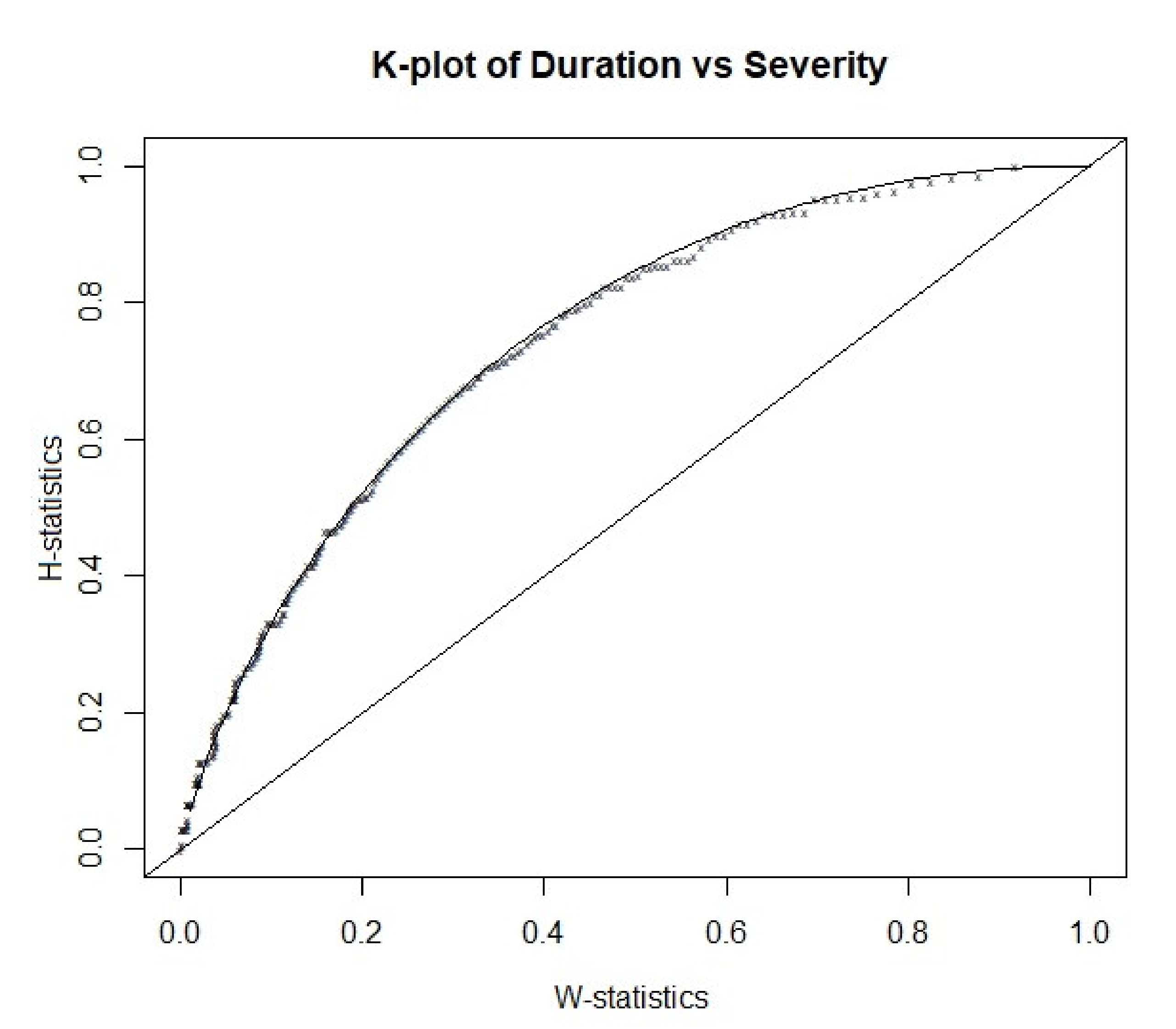
- Genest, C.; Boies, J.-C. Detecting dependence with Kendall plots. Am. Stat. 2003, 57, 275–284. [Google Scholar] [CrossRef]
- Xu, Y.; Huang, G.; Fan, Y. Multivariate flood risk analysis for Wei River. Stoch. Environ. Res. Risk Assess. 2015, 31, 225–242. [Google Scholar] [CrossRef]
- Kim, G.; Silvapulle, M.J.; Silvapulle, P. Comparison of semiparametric and parametric methods for estimating copulas. Comput. Stat. Data Anal. 2006, 51, 2836–2850. [Google Scholar] [CrossRef]


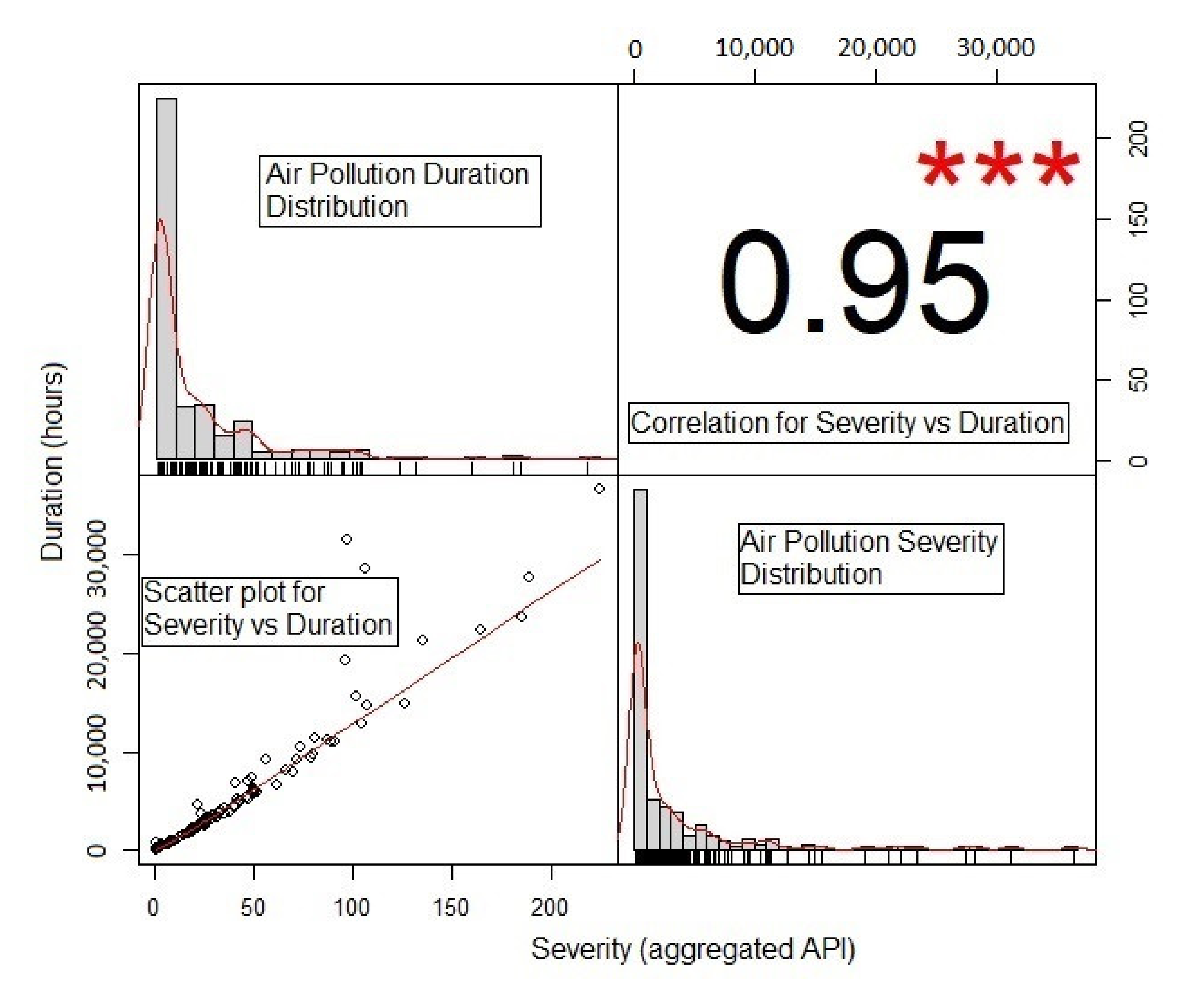
| Variable | Mean | Median | Min. Value | Max. Value | Std. Deviation | Skewness | Kurtosis |
|---|---|---|---|---|---|---|---|
| Duration (hours) | 21.39 | 3.00 | 1.00 | 224.00 | 64.81 | 2.78 | 9.23 |
| Severity | 2876.50 | 367.00 | 102.00 | 36,677.00 | 15,193.68 | 3.38 | 13.12 |
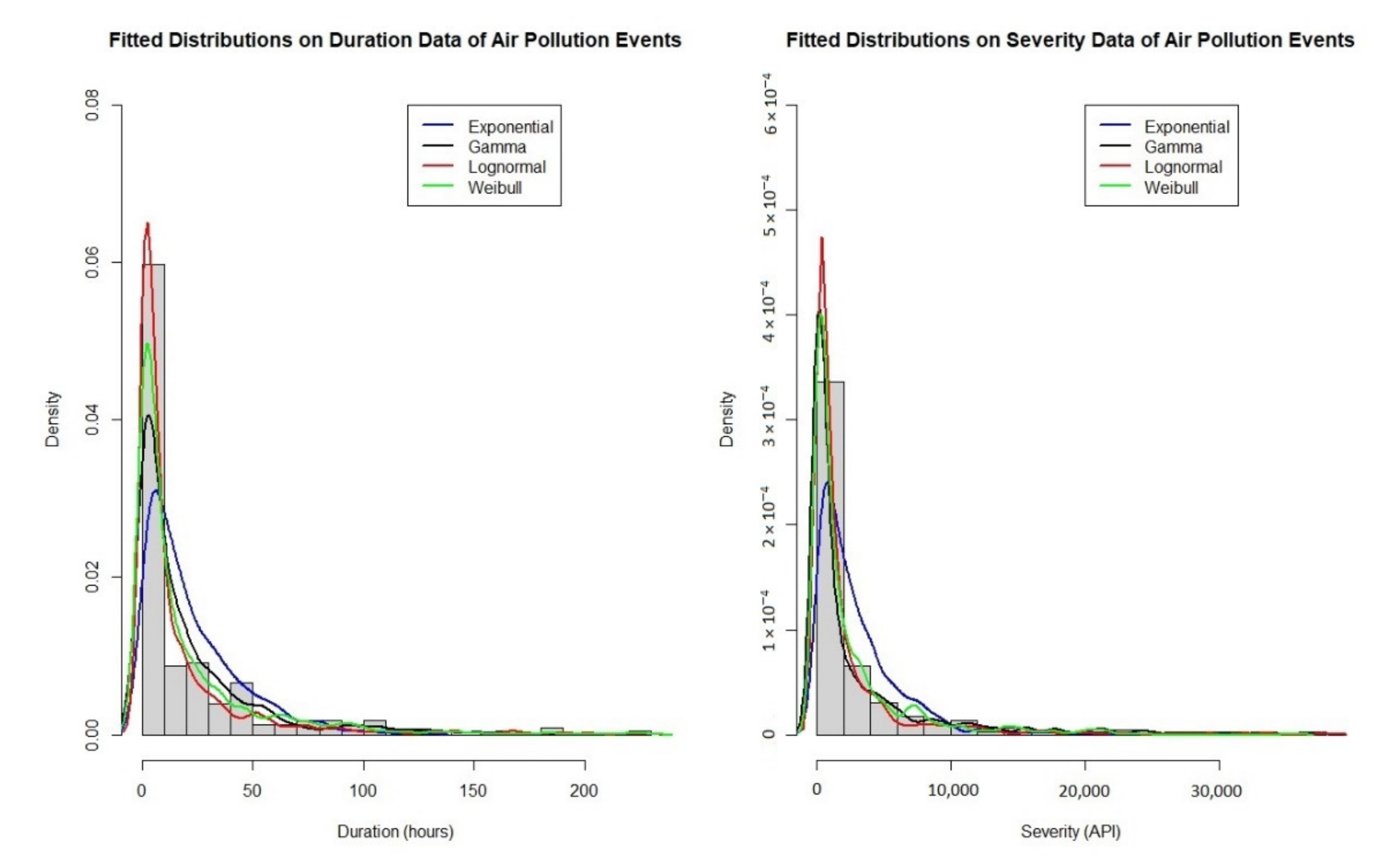
| Variable | Fitted Distribution | KS-Statistic | p-Value |
|---|---|---|---|
| Duration | Exponential | 0.3843 | 0.0000 |
| Gamma | 0.1834 | 0.0009 | |
| Lognormal | 0.1877 | 0.0006 | |
| Weibull | 0.2227 | 0.0002 | |
| Severity | Exponential | 0.3973 | 0.0000 |
| Gamma | 0.2969 | 0.0000 | |
| Lognormal | 0.1834 | 0.0009 | |
| Weibull | 0.2139 | 0.0005 |
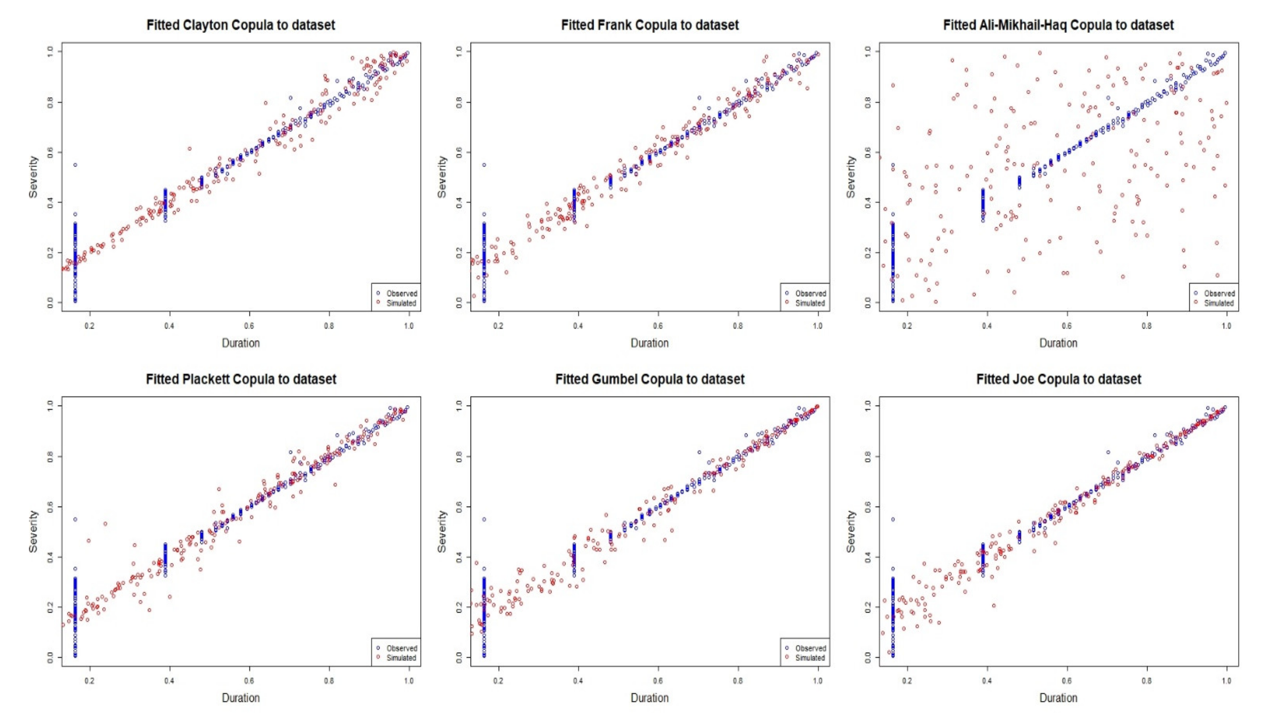
| Copula Model | Parameter Estimate (θ) | cVCIC | Kendall’s τ |
|---|---|---|---|
| Clayton | 22.85 | 49.108 | 0.9195 |
| Ali–Mikhail–Haq | 1 | 35.689 | 0.3333 |
| Frank | 48 | 142.708 | 0.9195 |
| Placket | 846.5 | 221.530 | 0.9195 |
| Gumbel | 12.42 | 199.361 | 0.9194 |
| Joe | 25.38 | 255.258 | 0.9195 |
| Duration Size | API Severity | Joint OR Return Period, (Days) | Joint AND Return Period, (Days) | Conditional D|S Return Period, (Days) | Conditional S|D Return Period, (Days) |
|---|---|---|---|---|---|
| 50-h | 100 | 4.4 | 34.4 | 34.6 | 268.5 |
| 1000 | 10.8 | 34.4 | 84.3 | 268.5 | |
| 10,000 | 34.4 | 56.4 | 720.9 | 439.9 | |
| 20,000 | 34.4 | 135.4 | 4153.6 | 1056.0 | |
| 30,000 | 34.4 | 406.3 | 4328.5 | 3168.0 | |
| 80-h | 100 | 4.4 | 56.4 | 56.7 | 721.1 |
| 1000 | 10.8 | 56.4 | 138.1 | 721.1 | |
| 10,000 | 54.8 | 58.2 | 743.2 | 743.2 | |
| 20,000 | 56.4 | 135.4 | 4153.6 | 1730.7 | |
| 30,000 | 56.4 | 406.3 | 7382.4 | 5192.0 | |
| 100-h | 100 | 4.4 | 101.6 | 102.0 | 2336.4 |
| 1000 | 10.8 | 101.6 | 248.6 | 2336.4 | |
| 10,000 | 56.4 | 101.6 | 1297.9 | 2336.4 | |
| 20,000 | 101.5 | 135.5 | 4153.9 | 3115.4 | |
| 30,000 | 101.6 | 406.3 | 7382.4 | 9345.6 | |
| 120-h | 100 | 4.4 | 169.3 | 170.0 | 6490.0 |
| 1000 | 10.8 | 169.3 | 414.2 | 6490.0 | |
| 10,000 | 56.4 | 169.3 | 2163.1 | 6490.0 | |
| 20,000 | 135.4 | 169.3 | 5193.5 | 6491.8 | |
| 30,000 | 169.3 | 406.3 | 7382.4 | 15,576.0 | |
| 150-h | 100 | 4.4 | 225.7 | 226.7 | 11,537.9 |
| 1000 | 10.8 | 225.7 | 552.3 | 11,537.9 | |
| 10,000 | 56.4 | 225.7 | 2884.1 | 11,537.9 | |
| 20,000 | 135.4 | 225.7 | 6922.7 | 11,537.9 | |
| 30,000 | 225.7 | 406.3 | 7382.4 | 20,768.1 |
Publisher’s Note: MDPI stays neutral with regard to jurisdictional claims in published maps and institutional affiliations. |
© 2021 by the author. Licensee MDPI, Basel, Switzerland. This article is an open access article distributed under the terms and conditions of the Creative Commons Attribution (CC BY) license (https://creativecommons.org/licenses/by/4.0/).
Share and Cite
Masseran, N. Modeling the Characteristics of Unhealthy Air Pollution Events: A Copula Approach. Int. J. Environ. Res. Public Health 2021, 18, 8751. https://doi.org/10.3390/ijerph18168751
Masseran N. Modeling the Characteristics of Unhealthy Air Pollution Events: A Copula Approach. International Journal of Environmental Research and Public Health. 2021; 18(16):8751. https://doi.org/10.3390/ijerph18168751
Chicago/Turabian StyleMasseran, Nurulkamal. 2021. "Modeling the Characteristics of Unhealthy Air Pollution Events: A Copula Approach" International Journal of Environmental Research and Public Health 18, no. 16: 8751. https://doi.org/10.3390/ijerph18168751