1. Introduction
The adverse impacts of ambient air pollution on human health and the ecosystem have been widely recognized [
1,
2]. At present, serious haze pollution—e.g., fine particulate matter (PM
2.5) and rebounded groun.cd−level ozone (O
3) pollution are the most concerning issues in China [
3,
4]. As one of the most important precursors of PM
2.5 and O
3 and key contributors to atmospheric oxidation, nitrogen dioxide (NO
2) plays key roles on both PM
2.5 and O
3 levels in complex air pollution [
5,
6,
7]. For this purpose, obtaining a thorough understanding of the trends of PM
2.5, O
3, and NO
2 is urgently needed.
Concentrations of these air pollutants are notably influenced by both emissions and meteorological conditions [
8,
9]. Although much effort has been made to tackle air pollutant emissions, severe air pollution events still occur under some stagnant meteorological conditions in China [
4]. An increase in the occurrence of O
3 pollution has been reported in the majority of cities in China, in contrast to decreases in PM
2.5 pollution levels [
10,
11]. Additionally, given the complex chemical reactions among primary air pollutants and relatively long life that allows for changing meteorological processes, variable levels of air pollutants can occur [
12,
13]. To successfully control air pollution, it is thus nontrivial to further identify the roles of distinct meteorological conditions on levels of air pollutants [
3,
14].
The Yangtze River Delta (YRD), an economically developed and densely populated area, is located on the east coast of China, comprising Shanghai City, Jiangsu Province, Zhejiang Province, and Anhui Province [
15]. Owing to rapid urbanization and industrialization, the YRD has experienced poor air quality in recent years. Many studies have investigated air pollution characteristics and their relationships with meteorological conditions in this area [
6,
16,
17]. Most previous studies investigating trends of surface air pollutants and meteorological impacts on them have been mainly carried out in one city or area of the YRD [
18,
19,
20,
21,
22]. Differences among regions in the YRD and influential factors have received relatively little attention, especially between coastal and inland cities. According to previous studies, atmospheric circulation, dispersion, and deposition can result in systematic differences in air pollutant concentrations between coastal and inland cities only a few hundred kilometers apart [
23,
24,
25]. However, these studies mainly involve short−term observations made in other parts of the country. The different characteristics of air pollutants between coastal and inland areas remain unclear, especially in the YRD. Studies based on simultaneously made long−term observations from coastal and inland cities are thus imperative to understand the impact of different geographical locations on the trends of surface air pollutants and their relationships with meteorological conditions in the YRD.
In this study, we investigated three main air pollutants, i.e., PM2.5, O3, and NO2, in a coastal city and an inland city in the YRD to gain insight into the influence of meteorological conditions on these air pollutants. Based on simultaneously measured long-term datasets of air pollutants and meteorological conditions from surface monitoring stations in Shanghai (SH) and Hefei (HF) from 2015 to 2019, the following issues are addressed: (1) the long-term trends of PM2.5, O3, and NO2 concentrations in coastal and inland cities; (2) the quantitative links between these air pollutant concentrations and meteorological variables in coastal and inland cities; and (3) the disparity in the impact of meteorological conditions in coastal and inland cities on the levels of air pollutants.
The paper is organized as follows: in
Section 2, we briefly describe the data measurement and analysis methods. In
Section 3, the long-trends of PM
2.5, O
3 and NO
2, the evolution of complex air pollution hours, and the influence of meteorological parameters on PM
2.5, O
3, and NO
2 are analyzed.
Section 4 provides the discussion and conclusions.
2. Data and Methods
2.1. Study Areas
Air pollutants, namely, PM
2.5, O
3, and NO
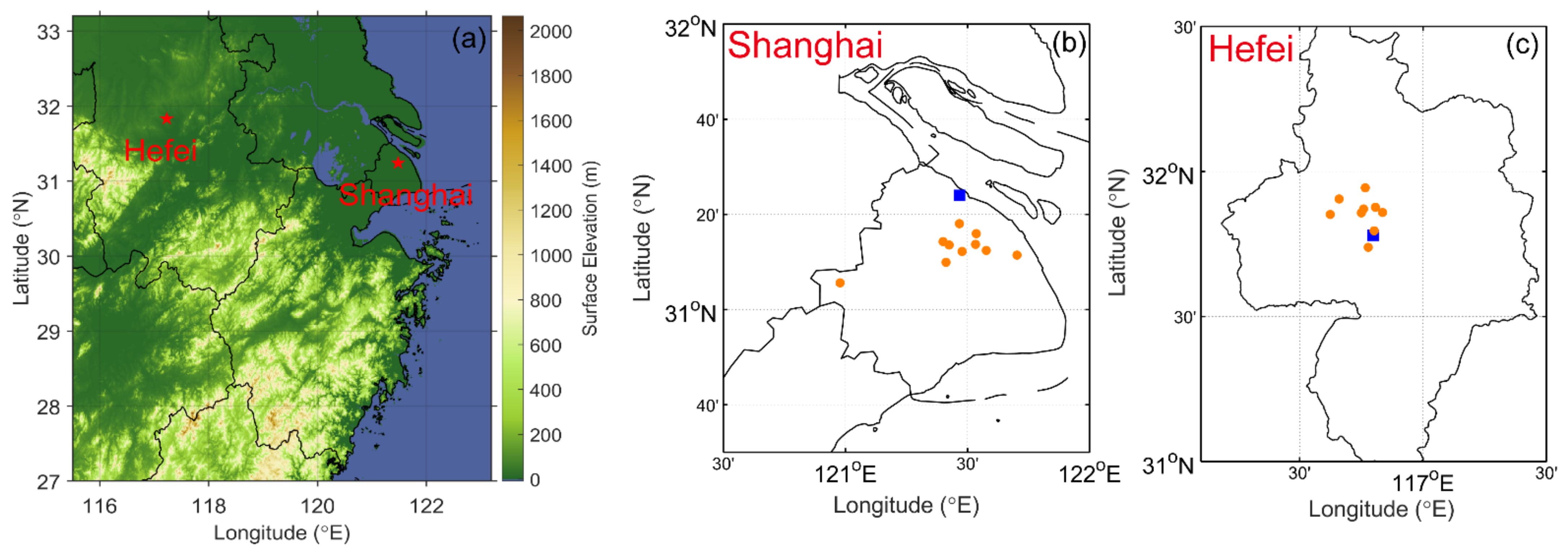
2, in a coastal city (SH) and an inland city (HF) in the YRD for the years 2015 to 2019 are investigated here (
Figure 1). SH (31°12′ N, 121°30′ E) is a representative coastal megacity located at the mouth of the YRD region, being a populous urban area and a national center of commerce, trade, and transportation, with the busiest container port in the world. HF (31°52′ N, 117°17′ E) is a typical inland city, about 450 km west of SH, and the capital of Anhui Province, bordering the North China Plain to the north, the Central China Region to the west, and the YRD to the east [
26]. HF is generally downwind of prevailing winds from the north and south in cold and warm seasons. In general, the coastal city of SH has better diffusion conditions than the inland city of HF. Air pollution deposition into the sea can largely reduce air pollutants near the coastal area as well [
24,
27]. Additionally, both cities feature a humid subtropical climate experiencing four distinct seasons. The complex monsoon and synoptic weather may have a substantial impact on air pollution formation and transport in this area [
18].
2.2. Data and Analysis Methods
Air pollutant and meteorological data were simultaneously collected in SH and HF from 1 January 2015 to 31 December 2019. Real-time, hourly concentrations of air pollutants, including PM
2.5, O
3, and NO
2, at all national air quality monitoring sites were published on an online platform published by the China National Environmental Monitoring Centre (CNEMC), while historical data is not openly available. We used historical data from 1 January 2015 to 31 December 2019 (at
https://quotsoft.net/air/ accessed on 15 February 2021) archived by one provider. Three−hourly meteorological data, i.e., air temperature (
T), dew-point temperature (
Td), atmospheric pressure (
P), wind speed and direction (
Ws, Wd), rainfall amount (
R), and horizontal visibility (
VIS), employed in this study are from the National Climate Data Center (
https://www.ncei.noaa.gov/data/global-hourly, accessed on 15 February 2021). Extreme high-temperature events were referred to days in which the daily maximum temperature is above 35 ℃. Relative humidity (
RH) is calculated from
T and
Td, based on the Clausius-Clapeyron equation. Wind directions are classified as the following: N, NNE, NE, ENE, E, ESE, SE, SSE, S, SSW, SW, WSW, W, WNW, NW, and NNW. Calm (C) condition is when
Ws ≤ 0.2 m/s. All the meteorological parameters were measured 8 times per day (3-h data) for each city. Considering that air pollutant and meteorological data are reported in Beijing Time (BJT) and Universal Time (UTC), respectively, converting UTC to BJT is required, i.e., BJT = UTC + 8 h.
A quality control process was conducted on the data at individual sites to remove problematic data points before calculating average concentrations and parameters. The citywide hourly mean concentrations of PM2.5, O3, and NO2 were calculated by averaging hourly data at all sites in the city, which were used in the analysis, as well as daily, seasonal, and annual mean concentrations. Three-hourly and daily mean meteorological parameters were also employed in this study. The high pollution periods under the joint impact of PM2.5 and O3 are defined as complex air pollution hours, and the thresholds of hourly mean concentration are 75 μg/m3 for PM2.5 and 200 μg/m3 for O3 based on the Ambient Air Quality Standard (GB3095−2012). Days with daily mean VIS < 10 km and RH < 90% were defined as hazy days according to the observation standard established by the China Meteorological Administration. Otherwise, a non−hazy day was recorded.
Seasons were defined as spring (March, April, and May), summer (June, July, and August), autumn (September, October, and November), and winter (December, January, and February). Regarding descriptive statistics, the least-squares regression method was used to derive the linear trends of the time series of air pollutant concentrations. The Pearson correlation analyses with a two-tailed student’s
t-test were chosen to evaluate the association between air pollutant concentrations and meteorological variables, which is known as the one of the best methods of measuring the relationship between variables. Due to the ability to provide valuable information about the predictor variables by removing or adding variables and high computation efficiency, for this step, the highest concentrations of O
3 wise multiple regression was adopted to assess the explained variances of the meteorological parameters on the variations in pollutants concentrations [
28,
29].
3. Results and Discussion
3.1. Long-Term Trends of PM2.5, O3, and NO2
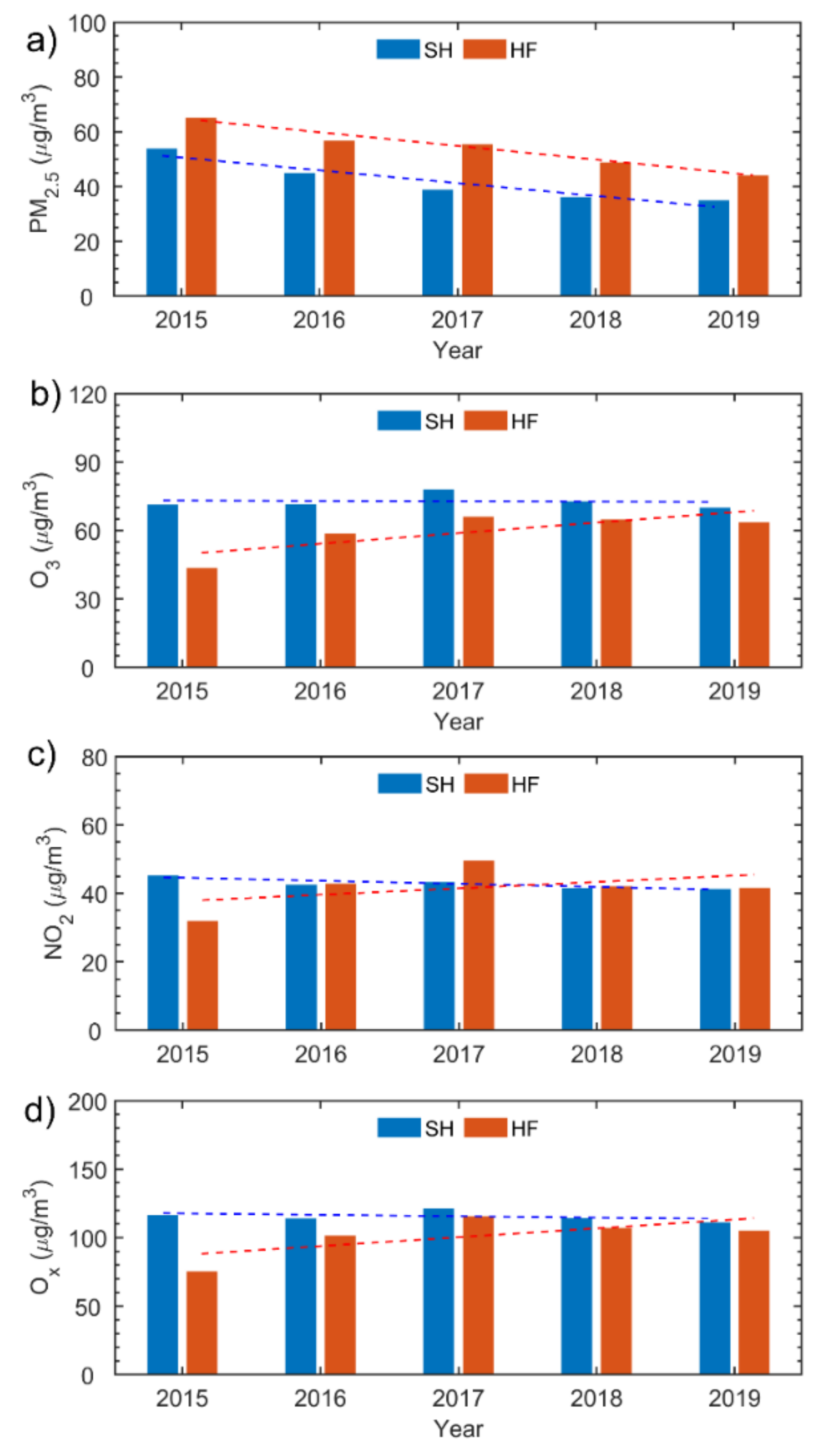
The long-term trends of annual mean concentrations of PM
2.5, O
3, and NO
2 were first investigated (
Figure 2). From 2015 to 2019, annual mean concentrations of PM
2.5 showed significant decreasing trends of −4.7% (
p < 0.05) in SH and of −5.0% (
p < 0.01) in HF as a result of the strict regional PM
2.5 reduction requirements. O
3 and NO
2 had fluctuating trends, initially increasing then decreasing slowly around 2017 in both SH and HF. However, O
3 and NO
2 showed net decreasing trends of −0.1% and −0.9% in SH, and net increasing trends of 4.6% and 1.9% in HF, respectively, which were insignificant at the 0.01 confidential level (
Figure 2 and
Table 1). The greatest frequency of the occurrence of extreme high-temperature events (28 days) in 2017 was to blame for the peak annual mean O
3 and NO
2 values that year. The trends for different seasons were also calculated (
Table 1). Both cities had decreasing trends for PM
2.5 in all seasons. The trends in summer and autumn in SH (
p < 0.05) and all seasons except autumn in HF (
p < 0.1) were statistically significant. As for O
3, NO
2, and O
x, in most seasons, trends slightly decreased (clearly increased) in SH (HF), which were mostly not statistically significant.
Furthermore, trends of the oxidant (O
x = O
3 + NO
2) were also investigated to evaluate the atmospheric oxidation capacities of distinct cities (
Figure 2d). As a comparison, the levels of PM
2.5 were much lower in SH while the levels of O
x were higher in SH than in HF over the entire study period. This suggests that local emissions from vehicle and industrial emissions were more dominant in the gases than PM
2.5 [
19]. Also revealed was the stronger atmospheric oxidation capacity in SH than in HF. The mean concentration of PM
2.5 in SH was 41.9 μg/m
3 over the whole study period, much lower than that in HF (54.1 μg/m
3), which might be due to the favorable diffusion conditions of the coastal location. However, the mean concentration of O
3 in SH was 72.8 μg/m
3, approximately 1.22 times that in HF (59.5 μg/m
3). Differences in NO
2 between the two cities were relatively smaller. Both coastal and inland PM
2.5 concentrations still exceeded the minimum safe level (annual mean <35 μg/m
3) for residential areas according to ambient air quality standards [
30]. Overall, the rates of decline of air pollutant concentrations have slowed down in both cities since 2017. This implies that improving air quality in the YRD remains a challenge.
The correlation between SH and HF daily mean air pollutants was further investigated. Moderately strong correlations between daily mean concentrations in SH and HF were obtained, with Pearson’s correlation coefficients of 0.58 (p < 0.01), 0.63 (p < 0.01), and 0.61 (p < 0.01) for PM2.5, O3, and NO2, respectively. These results suggest that not only the local emissions but also the coordinated regional emissions are crucial in making air pollutant control policies.
3.2. Evolution of Complex Air Pollution Hours
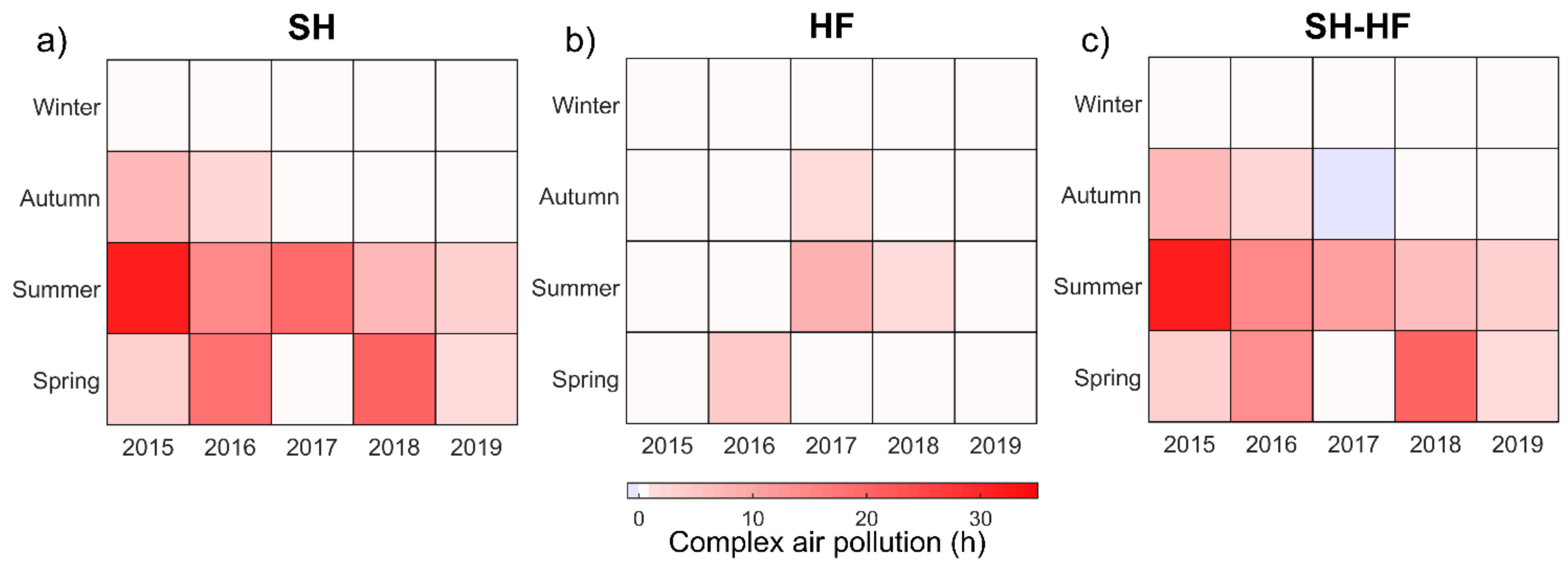
Figure 3 showed the evolution of complex air pollution hours with mean PM
2.5 concentration exceeding 75 μg/m
3 and O
3 exceeding 200 μg/m
3 simultaneously. In general, both cities had decreasing trends for the occurrence of complex air pollution over the period 2015–2019, although sometimes rebounded. The complex air pollution had a seasonal pattern, peaking in summer followed by spring and autumn. No complex polluted hour was found in winter. Distinct differences can be seen between each city. The complex air pollution in SH was worse with 127 h in 40 days than that of 14 h in 4 days in HF. Besides, the complex air pollution hours in SH are higher in most seasons except autumn in 2017 during the study period. This is likely due to hourly PM
2.5 and O
3 accumulation caused by the sea—land breeze convergences in SH [
31].
3.3. Influence of Meteorological Parameters on PM2.5, O3, and NO2
3.3.1. Overview of Correlations between Air Pollutants and Meteorological Parameters
The influence of meteorological parameters on concentrations of PM
2.5, O
3, and NO
2 was quantified using the Pearson correlation analysis (
Table 2). Calculated were the correlation coefficients between daily mean values of six meteorological parameters and three air pollutants in different seasons. Regarding similarities,
Ws was most negatively correlated with PM
2.5 and NO
2 concentrations in all seasons in the two cities, indicating its important role in the dispersion of air pollutants.
R was most related to PM
2.5 due to wet deposition by heavy rain, while the relationship with NO
2 was not significant. The influence of different rainfall categories on air pollutants is investigated in
Section 3.3.3.
T was weakly correlated with PM
2.5 and NO
2 concentrations in almost all seasons.
In contrast with PM
2.5 and NO
2,
T, and
RH (followed by
Ws) were the most closely correlated with O
3. The O
3 correlations with
T were positive due to accelerated O
3 production under high-temperature conditions accelerating photochemical reaction rates, with strong correlations in winter, autumn, and summer. Significant negative correlations between O
3 concentrations and
RH were found throughout the year in both cities due to the crucial role water vapor played in decreasing photochemical ozone production by affecting solar ultraviolet radiation [
32]. Warm, dry weather is thus more conducive to O
3 formation than cool, wet weather. The impact of
Ws on O
3 concentrations was complex, showing weaker correlations in all seasons, respectively. This likely resulted from the simultaneous diffusion and vertical mixing effect. Normally, it’s conducive to the build-up of O
3 formation with stronger vertical mixing and weaker diffusion, however, weaker vertical mixing and stronger diffusion decreased O
3 concentrations [
33].
Section 3.3.2 comprehensively analyzes the relationships between air pollutants and
Ws/
Wd.
Concerning differences in the meteorological influence on air pollutants between both cities, Ws and Wd had stronger relationships with all air pollutants in SH than in HF. T had a weaker relationship with O3 in SH. In general, these results are primarily attributed to different meteorological and diffusion conditions experienced by coastal and inland areas.
The explained variance of six meteorological parameters upon the daily variability of PM
2.5, O
3, and NO
2 in different seasons was calculated using a step-wise multiple linear regression method (
Table 3). The six meteorological factors together can explain higher variances of summertime and autumntime daily levels of PM
2.5 (O
3, NO
2) in SH and HF, respectively. This suggests that meteorological factors play essential roles in the daily fluctuations of pollutants in summer. Note that the explained variances were generally higher in summer and autumn than in other seasons. Moreover, the explained variances of all air pollutants derived in SH were significantly higher than those in HF in all seasons except for O
3 in spring and summer. This implies the stronger influence of meteorological parameters in the coastal area.
3.3.2. PM2.5, O3, and NO2 Concentrations for Different Wind Directions and Speeds
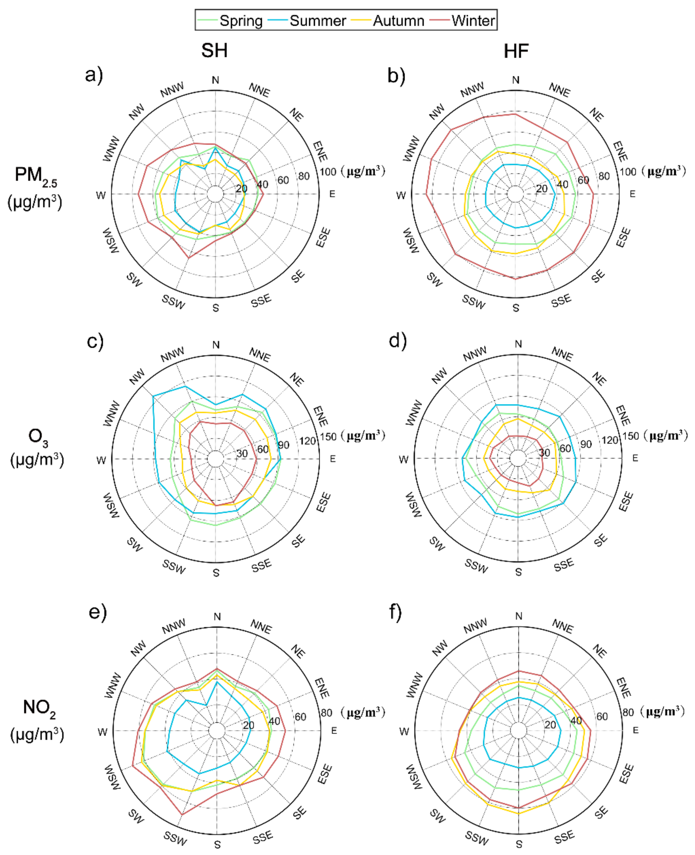
To better illustrate the influence of wind direction on pollutants,
Figure 4 shows seasonal mean concentrations of PM
2.5, O
3, and NO
2 for different wind directions. In general, all air pollutants were distributed more evenly in HF in all seasons than in SH. PM
2.5 and NO
2 concentrations in SH were the highest when the wind came from the westerly direction (i.e., W, WSW, and SSW), followed by northerly winds in most seasons, consistent with a previous study [
20,
30]. This suggests the contribution of transported air pollutants to air pollution episodes in SH was from the west and the north, while the air from the east and south sea was much cleaner with lower emissions. In all seasons, NW winds in SH led to the highest O
3 concentrations, followed by NE winds. O
3 concentrations varied little in other wind directions.
By contrast, in HF, peak values of PM2.5 concentration were associated with NW, SE and SSW winds, and O3 and NO2 maximum concentrations were associated with SE winds. However, in all seasons, Wd did not play an important role in changing the concentrations of the three air pollutants in HF as it did in SH. The highest concentrations of PM2.5 and NO2 occurred in winter, and the highest concentrations of O3 occurred in summer for all directions in HF, which demonstrated again the positive correlation between O3 and temperature.
Seasonal mean concentrations of PM
2.5, O
3, and NO
2 under calm conditions were also examined, along with the ratios PM
2.5/CO, O
3/CO, and NO
2/CO as indicators of air pollutant secondary formation to primary emissions (
Table 4). PM
2.5 and NO
2 concentrations were higher, and O
3 concentrations were much lower under calm conditions than under windy conditions in both cities, i.e., calm conditions were favorable for the accumulation of PM
2.5 and NO
2 but unfavorable for O
3 formation in both coastal and inland cities. As a comparison, the concentrations of PM
2.5 under calm conditions were lower, and O
3 concentrations were much higher in SH than in HF in almost all seasons. Three possible reasons are: (1) There was much lower (higher) PM
2.5 (O
3 precursors) emissions in SH than in HF according to the Emission Inventory for China (MEIC v1.3,
http://meicmodel.org, accessed on 12 August 2021) [
34,
35]; and (2) Lower PM
2.5/CO and higher O
3/CO ratios were found in SH than in HF, revealing weakened PM
2.5 formation and enhanced O
3 formation from primary emissions in SH under calm conditions; and (3) Sea−breeze was noticeable resulting in a cycling pattern under the calm wind condition while was not significant under the strong wind condition of prevailing winds in SH [
36].
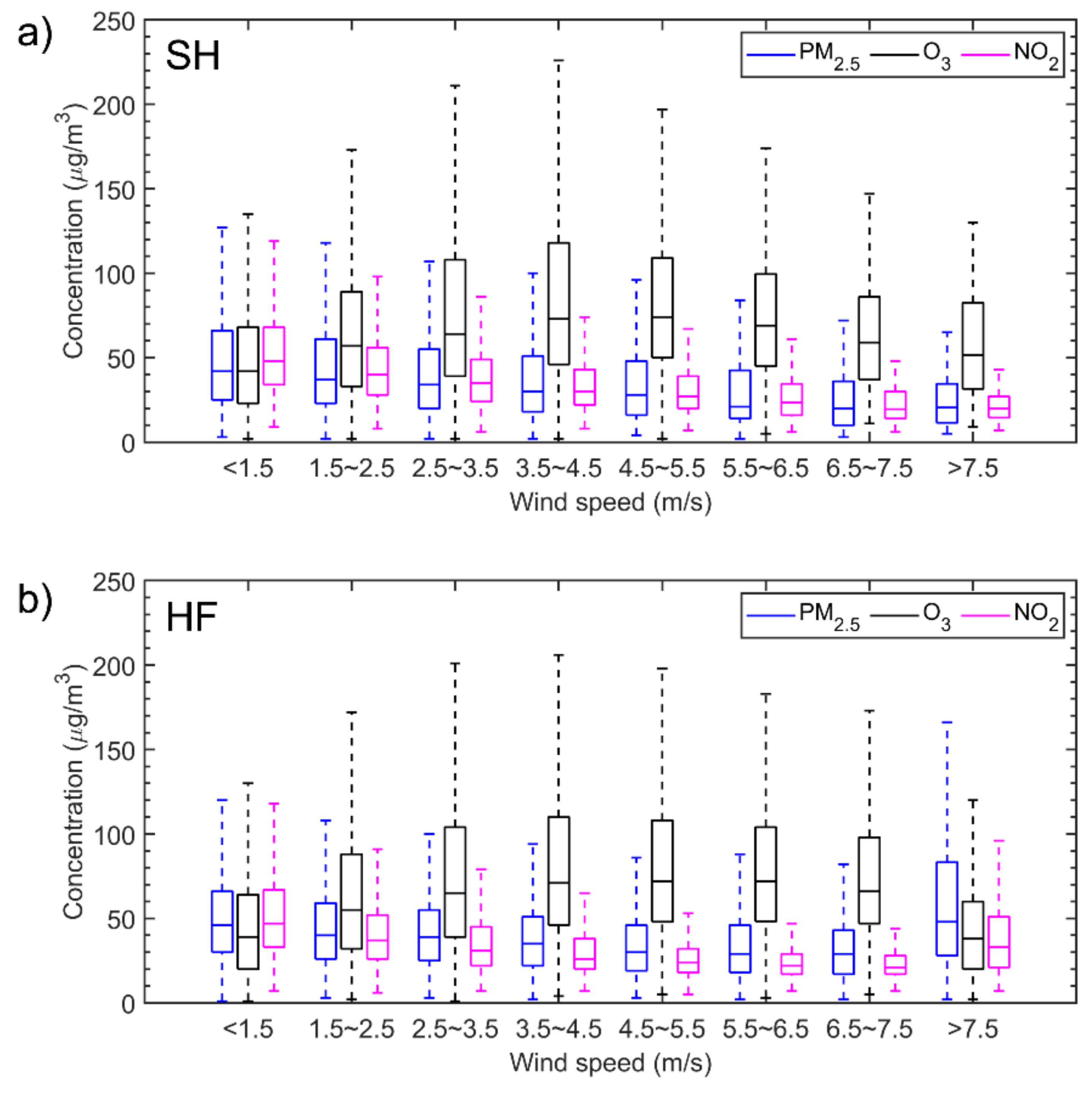
Figure 5 shows hourly mean concentrations of PM
2.5, O
3, and NO
2 in each category of wind speed in SH and HF. Both cities show similar relationships between pollutant concentrations and wind speed. In general, for wind speeds below 7.5 m/s, PM
2.5 and NO
2 concentrations decreased as wind speeds increased. This is because high winds tend to disperse air pollutants and dilute PM
2.5 and NO
2 concentrations, while stagnant conditions and light winds allow them to build up and become more concentrated. When wind speeds exceeded 7.5 m/s in HF, regional transport might have played a greater role than air dispersal. Concentrations of O
3 increased to a peak value when wind speeds were between 3.5 and 4.5 m/s, then gradually decreased. These results are mainly ascribed to two simultaneous effects. Higher wind speeds increase air turbulence and facilitate the vertical mixing of upper-level O
3 to the ground. Higher wind speeds also have a diffusion effect, diluting O
3 concentrations. When wind speeds are lower, the mixing effect of O
3 concentration is stronger than the diffusion effect. As wind speeds exceed a threshold value, the diffusion effect dominates again [
37].
3.3.3. PM2.5, O3, and NO2 Concentrations for Different Rainfall Categories
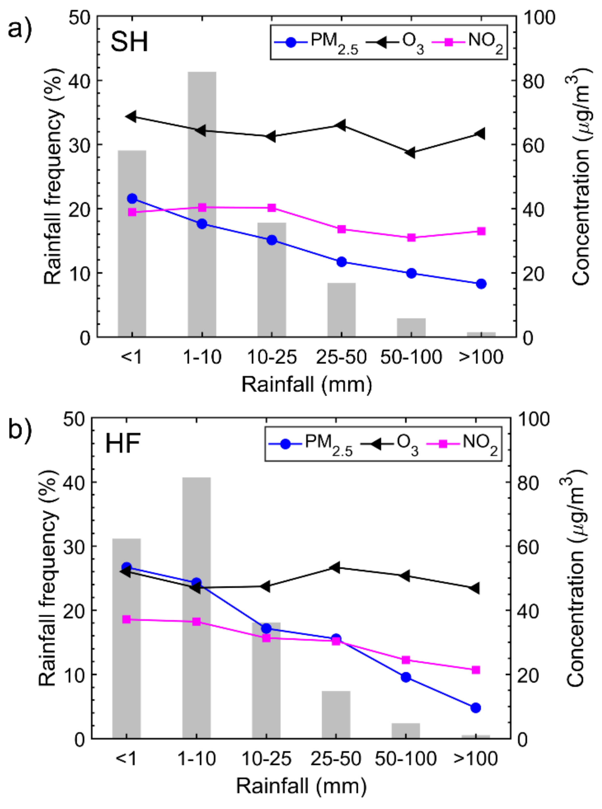
Like dispersion and transportation, wet deposition plays a substantial role in modifying air pollutants. Examined next is the influence of daily rainfall scavenging on changes in PM
2.5, O
3, and NO
2 concentrations (
Figure 6). At both sites, concentrations of PM
2.5 were greatly reduced. However, the reduction in O
3 and NO
2 (gaseous pollutants) was lower than that of PM
2.5. The relative effect of rainfall washout on air pollutant concentrations is estimated to be PM
2.5 > NO
2 > O
3. An interesting phenomenon occurred for O
3 and NO
2. Their concentrations tended to increase somewhat under rainy conditions. This is likely due to vertical mixing, bringing down a certain amount of O
3 and NO
2 from the upper layers of the atmosphere during convective rain activity and thunderstorms [
38,
39,
40,
41,
42]. Surface NO
2 concentrations can also be enhanced by lightning-generated NO
2 during convective rain events [
43,
44,
45]. Rainfall frequency distributions in the two cities were similar, with the highest frequency occurring when the daily rainfall intensity was 1–10 mm. The washout effect for PM
2.5 and NO
2 was more effective in HF than in SH, likely due to the greater frequency of strong convection and thunderstorms in inland areas than in coastal areas [
46,
47]. Concerning O
3, the washout effect was limited in both cities. Different patterns in O
3 concentration occurred in SH and HF when the daily rainfall intensity exceeded 25 mm.
3.3.4. PM2.5, O3, and NO2 Concentrations on Hazy and Non−hazy Days
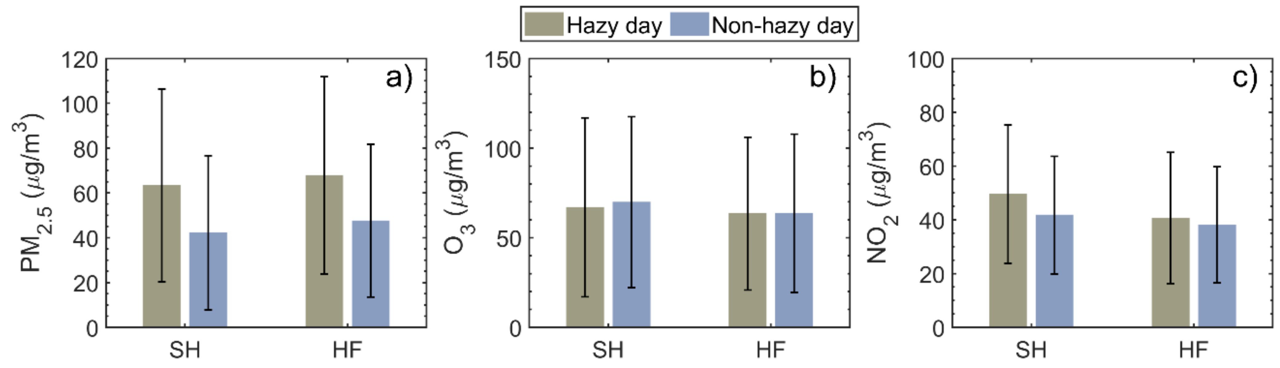
Figure 7 shows daily mean concentrations of PM
2.5, O
3, and NO
2 on hazy days and non−hazy days, calculated using long-term observational data from 2015 to 2019. PM
2.5 concentrations were higher on hazy days in both cities, i.e., 63.4 and 67.8 μg/m
3 in SH and HF, respectively, than on non-hazy days, i.e., 42.2 and 47.6 μg/m
3 in SH and HF, respectively. This amounts to an increase in PM
2.5 concentration of 50.2% and 42.4% in SH and HF, respectively, mainly due to weakened surface winds, high
RH, and a low PBL, promoting the accumulation of PM
2.5 and hygroscopic growth on hazy days. Note that PM
2.5 concentrations on 34.9% (SH) and 34.4% (HF) of hazy days were greater than 75 μg/m
3 (the standard for a polluted day), indicating that hazy days remain a major air pollution problem in both coastal and inland cities. Similar results were found for NO
2, but the differences in NO
2 concentrations between hazy and non-hazy days were much smaller.
By contrast, O
3 concentrations were 4.3% and 0.3% higher on non−hazy days than on hazy days in SH and HF, respectively. The suppression of photochemical reactions resulting from reduced sunshine on hazy days, particularly in SH, likely explains this. Higher levels of PM
2.5 and lower levels of O
3 and NO
2 were found in HF compared with SH on both hazy and non−hazy days. These results are consistent with the annual and seasonal trends shown in
Figure 2 and
Figure 3.
4. Conclusions
HF represents a typical inland city located about 450 km west of the typical coastal city of SH, making it a useful model for understanding the influence of different locations on air pollutants in the YRD region. In this study, the contrasting trends of surface PM2.5, O3, and NO2 and their relationships with meteorological parameters in SH and HF were investigated based on surface air pollutant and meteorological datasets from 2015 to 2019. We provide the following conclusions:
In both cities, significant decreasing trends were observed for PM2.5, while O3 and NO2 fluctuated with turning points during 2017 when the most frequent extreme high−temperature events occurred. The rate of decrease in air pollutants slowed in both cities, demonstrating the challenge of persistent reduction in air pollution. Compared with HF, PM2.5 concentrations were much lower, Ox (O3+NO2) levels were higher, and the complex air pollution was worse in SH. The correlations of air pollutants between SH and HF were 0.58 (p < 0.01), 0.63 (p < 0.01), and 0.61 (p < 0.01) for PM2.5, O3, and NO2, respectively, indicating that approximately 60% of time both cities are affected by similar atmospheric conditions due to common regional meteorology.
Considerably different correlations between air pollutants and meteorological parameters were observed, given the diversity of meteorological conditions in both cities. In both cities, Ws was negatively correlated with PM2.5 and NO2 concentrations, followed by T and R. Most closely related to O3 were T (positive correlation) and RH (negative correlation), followed by Ws. Compared with HF, Ws and Wd had stronger relationships with all air pollutants while T had a weaker relationship with O3 in SH, likely due to different sea−land meteorological and diffusion conditions experienced by coastal and inland areas. The six meteorological factors together can explain 68.7% (51.7%, 72.4%) and 56.6% (67.5%, 43.1%) of the variances of summertime daily levels of PM2.5 (O3, NO2) in SH and HF, respectively. Summertime correlation coefficients and explained variances were generally higher than those in other seasons.
Air pollutant concentrations changed more with Wd possibly due to the limit imposed by the shoreline in SH than in HF, where Wd did not play as much of a role in changing air pollutant concentrations. Westerly winds led to the highest PM2.5 and NO2 concentrations, while NW winds were associated with the highest O3 concentrations in SH. In both cities, PM2.5 and NO2 concentrations showed decreasing trends as a function of Ws under most conditions. O3 concentrations increased to a peak value, then gradually decreased. Windless conditions were favorable for PM2.5 and NO2 but adverse to O3 formation in both coastal and inland cities. PM2.5 (O3) concentrations were lower (higher) in SH than in HF under calm conditions.
All air pollutant concentrations were reduced by rainfall scavenging, with the greatest reduction seen in PM2.5, followed by NO2 and O3. A more effective washout effect was observed in HF, mostly because of the more frequent strong convection and thunderstorms in this inland area. Interestingly, O3 and NO2 concentrations tended to somewhat increase under rainy conditions in both cities, likely due to convection and lightning, respectively.
A similar increase in PM2.5 and NO2 concentrations occurred on hazy days compared to non−hazy days. However, O3 had higher concentrations on non−hazy days, likely due to the suppression of photochemical reactions resulting from reduced sunshine in the presence of haze. HF had higher levels of PM2.5 and lower levels of O3 and NO2 compared with SH on both hazy and non−hazy days. Further studies of air pollution at coastal and inland sites in other regions of China, as well as the detailed investigations of specific events to learn more about the physical processes leading to the observed differences between coastal and inland cities, are needed to obtain a deeper, more comprehensive understanding of the nationwide air quality problem.
Author Contributions
Conceptualization, M.L.; Q.J. and Z.L.; Methodology, M.L. and T.C.; data curation and investigation, M.L.; T.C.; Y.W. and A.C.; Validation, A.H. and T.C.; Writing—original draft preparation, M.L.; Writing—review and editing, M.C. All authors have read and agreed to the published version of the manuscript.
Funding
This work was supported by the Research Startup Foundation of Nantong University (No. 03081212) and the Nantong Basic Scientific Research Program (No. JC2020167).
Data Availability Statement
The long-term air quality monitoring datasets in SH and HF analyzed during the current study are available from
https://quotsoft.net/air/ (accessed on 15 February 2021). The meteorological data were obtained from the US National Centers for Environment Prediction’s Global Data Assimilation System (
ftp://arlftp.arlhq.noaa.gov/pub/archives/gdas1, accessed on 15 February 2021).
Acknowledgments
The authors acknowledge the China National Environmental Monitoring Centre (CNEMC) and National Oceanic and Atmospheric Administration (NOAA) for the data that they kindly provided.
Conflicts of Interest
The authors declare no conflict of interest.
References
- Héroux, M.E.; Anderson, H.R.; Atkinson, R.; Brunekreef, B.; Cohen, A.; Forastiere, F.; Hurley, F.; Katsouyanni, K.; Krewski, D.; Krzyzanowski, M.; et al. Quantifying the health impacts of ambient air pollutants: Recommendations of a WHO/Europe project. Int. J. Public Health. 2015, 60, 619–627. [Google Scholar] [CrossRef] [PubMed] [Green Version]
- Ricciardelli, I.; Bacco, D.; Rinaldi, M.; Bonafe’, G.; Scotto, F.; Trentini, A.; Bertacci, G.; Ugolini, P.; Zigola, C.; Rovere, F.; et al. A three–year investigation of daily PM2.5 main chemical components in four sites: The routine measurement program of the Supersito Project (Po Valley, Italy). Atmos. Environ. 2017, 152, 418–430. [Google Scholar] [CrossRef]
- Wang, P.; Guo, H.; Hu, J.; Kota, S.H.; Ying, Q.; Zhang, H. Responses of PM2.5 and O3 concentrations to changes of meteorology and emissions in China. Sci. Total Environ. 2019, 662, 297–306. [Google Scholar] [CrossRef] [PubMed]
- Zhao, S.; Yin, D.; Yu, Y.; Kang, S.; Qin, D.; Dong, L. PM2.5 and O3 pollution during 2015–2019 over 367 Chinese cities: Spatiotemporal variations, meteorological and topographical impacts. Environ. Pollut. 2020, 264, 114694. [Google Scholar] [CrossRef]
- Gao, W.; Tie, X.; Xu, J.; Huang, R.; Mao, X.; Zhou, G.; Chang, L. Long–term trend of O3 in a megacity (Shanghai), China: Characteristics, causes, and interactions with precursors. Sci. Total Environ. 2017, 603, 425–433. [Google Scholar] [CrossRef]
- Li, L.; Lu, C.; Chan, P.W.; Zhang, X.; Yang, H.L.; Lan, Z.; Zhang, W.H.; Liu, Y.W.; Pan, L.; Zhang, L. Tower observed vertical distribution of PM2.5, O3 and NOx in the Pearl River Delta. Atmos. Environ. 2020, 220, 117083. [Google Scholar] [CrossRef]
- Chu, B.; Ma, Q.; Liu, J.; Ma, J.; Zhang, P.; Chen, T.; Feng, Q.; Wang, C.; Yang, N.; Ma, J.; et al. Air pollutant correlations in China: Secondary air pollutant responses to NOx and SO2 control. Environ. Sci. Technol. Let. 2020, 7, 695–700. [Google Scholar] [CrossRef]
- Zhang, Q.; Ma, Q.; Zhao, B.; Liu, X.; Wang, Y.; Jia, B.; Zhang, X. Winter haze over North China Plain from 2009 to 2016: Influence of emission and meteorology. Environ. Pollut. 2018, 242, 1308–1318. [Google Scholar] [CrossRef]
- An, Z.; Huang, R.J.; Zhang, R.; Tie, X.; Li, G.; Cao, J. Severe haze in northern China: A synergy of anthropogenic emissions and atmospheric processes. Proc. Natl. Acad. Sci. USA 2019, 116, 8657–8666. [Google Scholar] [CrossRef] [Green Version]
- Sun, L.; Xue, L.; Wang, T.; Gao, J.; Ding, A.; Cooper, O.R.; Lin, M.; Xu, P.; Wang, Z.; Wang, X.; et al. Significant increase of summertime ozone at Mount Tai in Central Eastern China. Atmos. Chem. Phys. 2016, 16, 10637–10650. [Google Scholar] [CrossRef] [Green Version]
- Wang, T.; Xue, L.; Brimblecombe, P.; Lam, Y.F.; Li, L.; Zhang, L. Ozone pollution in China: A review of concentrations, meteorological influences, chemical precursors, and effects. Sci. Total Environ. 2017, 575, 1582–1596. [Google Scholar] [CrossRef]
- Zhao, H.Y.; Zhang, Q.; Guan, D.B.; Davis, S.J.; Liu, Z.; Huo, H.; Lin, J.T.; Liu, W.D.; He, K.B. Assessment of China’s virtual air pollution transport embodied in trade by using a consumption–based emission inventory. Atmos. Chem. Phys. 2015, 15, 5443–5456. [Google Scholar] [CrossRef] [Green Version]
- Cepeda, M.; Schoufour, J.; Freak–Poli, R.; Koolhaas, C.M.; Dhana, K.; Bramer, W.M.; Franco, O.H. Levels of ambient air pollution according to mode of transport: A systematic review. Lancet Public Health 2017, 2, 23–34. [Google Scholar] [CrossRef] [Green Version]
- Peng, L.; Zhao, X.; Tao, Y.; Mi, S.; Huang, J.; Zhang, Q. The effects of air pollution and meteorological factors on measles cases in Lanzhou, China. Environ. Sci. Pollut. R. 2020, 27, 13524–13533. [Google Scholar] [CrossRef]
- Wang, H.; Zhang, Y.; Tsou, J.Y.; Li, Y. Surface urban heat island analysis of Shanghai (China) based on the change of land use and land cover. Sustainability 2017, 9, 1538. [Google Scholar] [CrossRef] [Green Version]
- Ma, T.; Duan, F.; He, K.; Qin, Y.; Tong, D.; Geng, G.; Liu, X.; Li, H.; Yang, S.; Ye, S.; et al. Air pollution characteristics and their relationship with emissions and meteorology in the Yangtze River Delta region during 2014–2016. J. Environ. Sci. 2019, 83, 8–20. [Google Scholar] [CrossRef]
- Yang, X.; Jiang, L.; Zhao, W.; Xiong, Q.; Zhao, W.; Yan, X. Comparison of ground–based PM2.5 and PM10 concentrations in China, India, and the US. Int. J. Environ. Res. Public Health 2018, 15, 1382. [Google Scholar] [CrossRef] [Green Version]
- Ding, A.J.; Fu, C.B.; Yang, X.Q.; Sun, J.N.; Zheng, L.F.; Xie, Y.N.; Herrmann, E.; Nie, W.; Petäjä, T.; Kerminen, V.M.; et al. Ozone and fine particle in the western Yangtze River Delta: An overview of 1–yr data at the SORPES station. Atmos. Chem. Phys. 2013, 13, 5813–5830. [Google Scholar] [CrossRef] [Green Version]
- Hu, J.; Wang, Y.; Ying, Q.; Zhang, H. Spatial and temporal variability of PM2.5 and PM10 over the North China Plain and the Yangtze River Delta, China. Atmos. Environ. 2014, 95, 598–609. [Google Scholar] [CrossRef]
- Wang, H.L.; Qiao, L.P.; Lou, S.R.; Zhou, M.; Ding, A.J.; Huang, H.Y.; Chen, J.M.; Wang, Q.; Tao, S.K.; Chen, C.H.; et al. Chemical composition of PM2.5 and meteorological impact among three years in urban Shanghai, China. J. Clean. Prod. 2016, 112, 1302–1311. [Google Scholar] [CrossRef]
- Gao, D.; Xie, M.; Chen, X.; Wang, T.; Liu, J.; Xu, Q.; Mu, X.; Chen, F.; Li, S.; Zhuang, B.; et al. Systematic classification of circulation patterns and integrated analysis of their effects on different ozone pollution levels in the Yangtze River Delta Region, China. Atmos. Environ. 2020, 242, 117760. [Google Scholar] [CrossRef]
- Liu, X.; Zhu, B.; Kang, H.; Hou, X.; Gao, J.; Kuang, X.; Yan, S.; Shi, S.; Fang, C.; Pan, C.; et al. Stable and transport indices applied to winter air pollution over the Yangtze River Delta, China. Environ. Pollut. 2021, 272, 115954. [Google Scholar] [CrossRef]
- Darby, L.S.; McKeen, S.A.; Senff, C.J.; White, A.B.; Banta, R.M.; Post, M.J.; Brewer, W.; Marchbanks, R.; Alvare, R.; Peckham, S.; et al. Ozone differences between near-coastal and offshore sites in New England: Role of meteorology. J. Geophys. Res. 2007, 112, 1–17. [Google Scholar] [CrossRef] [Green Version]
- Tian, Y.; Liu, J.; Han, S.; Shi, X.; Shi, G.; Xu, H.; Yu, H.; Zhang, Y.; Feng, Y.; Russell, A. Spatial, seasonal and diurnal patterns in physicochemical characteristics and sources of PM2.5 in both coastal and inland regions within a megacity in China. J. Hazard. Mater. 2018, 342, 139–149. [Google Scholar] [CrossRef]
- Wei, M.; Liu, H.; Chen, J.; Xu, C.; Li, J.; Xu, P.; Sun, Z. Effects of aerosol pollution on PM2.5—Associated bacteria in typical coastal and inland cities of northern China during the winter heating season. Environ. Pollut. 2020, 262, 114188. [Google Scholar] [CrossRef]
- Huang, L.; Chen, M.; Hu, J. Twelve–year trends of PM10 and visibility in the Hefei metropolitan area of China. Adv. Meteorol. 2016, 2016, 4810796. [Google Scholar] [CrossRef] [Green Version]
- Viana, M.; Hammingh, P.; Colette, A.; Querol, X.; Degraeuwe, B.; de Vlieger, I.; van Aardenne, J. Impact of maritime transport emissions on coastal air quality in Europe. Atmos. Environ. 2014, 90, 96–105. [Google Scholar] [CrossRef]
- Ilten, N.; Selici, A.T. Investigating the impacts of some meteorological parameters on air pollution in Balikesir, Turkey. Environ. Monit. Assess. 2008, 140, 267–277. [Google Scholar] [CrossRef]
- Zhai, S.; Jacob, D.J.; Wang, X.; Shen, L.; Li, K.; Zhang, Y.; Gui, K.; Zhao, T.; Liao, H. Fine particulate matter (PM2.5) trends in China, 2013–2018: Separating contributions from anthropogenic emissions and meteorology. Atmos. Chem. Phys. 2019, 19, 11031–11041. [Google Scholar] [CrossRef] [Green Version]
- Zhang, Z.; Zhang, X.; Gong, D.; Quan, W.; Zhao, X.; Ma, Z.; Kim, S.J. Evolution of surface O3 and PM2.5 concentrations and their relationships with meteorological conditions over the last decade in Beijing. Atmos. Environ. 2015, 108, 67–75. [Google Scholar] [CrossRef]
- Mao, Z.; Xu, J.; Yang, D.; Yu, Z.; Zhai, Y.; Zhou, G. Analysis of characteristics and meteorological causes of PM2.5–O3 compound pollution in Shanghai. Chin. Environ. Sci. 2019, 39, 2730–2738. [Google Scholar]
- Bais, A.F.; Lucas, R.M.; Bornman, J.F.; Williamson, C.E.; Sulzberger, B.; Austin, A.T.; Wilson, S.R.; Andrady, A.L.; Bernhard, G.; McKenzie, R.L.; et al. Environmental effects of ozone depletion, UV radiation and interactions with climate change: UNEP Environmental Effects Assessment Panel, update 2017. Photoch. Photobio. Sci. 2018, 17, 127–179. [Google Scholar] [CrossRef] [PubMed]
- Shi, Z.; Huang, L.; Li, J.; Ying, Q.; Zhang, H.; Hu, J. Sensitivity analysis of the surface ozone and fine particulate matter to meteorological parameters in China. Atmos. Chem. Phys. 2020, 20, 13455–13466. [Google Scholar] [CrossRef]
- Chen, C.; Wang, B.; Fu, Q.; Green, C.; Streets, D.G. Reductions in emissions of local air pollutants and co–benefits of Chinese energy policy: A Shanghai case study. Energ. Policy. 2006, 34, 754–762. [Google Scholar]
- Zheng, B.; Tong, D.; Li, M.; Liu, F.; Hong, C.; Geng, G.; Li, H.; Li, X.; Peng, L.; Qi, J.; et al. Trends in China’s anthropogenic emissions since 2010 as the consequence of clean air actions. Atmos. Chem. Phys. 2018, 18, 14095–14111. [Google Scholar] [CrossRef] [Green Version]
- Tie, X.; Geng, F.; Peng, L.; Gao, W.; Zhao, C. Measurement and modeling of O3 variability in Shanghai, China: Application of the WRF–Chem model. Atmos. Environ. 2009, 43, 4289–4302. [Google Scholar] [CrossRef]
- An, J.; Wang, Y.; Sun, Y. Assessment of ozone variations and meteorological effects in Beijing. Ecol. Environ. Sci. 2009, 18, 944–951. [Google Scholar]
- Muralidharan, V.; Kumar, G.M.; Sampath, S. Surface ozone variation associated with rainfall. Pure Appl. Geophys. 1989, 130, 47–55. [Google Scholar] [CrossRef]
- Jain, S.L.; Arya, B.C.; Kumar, A.; Ghude, S.D.; Kulkarni, P.S. Observational study of surface ozone at New Delhi, India. Int. J. Remote Sens. 2005, 26, 3515–3524. [Google Scholar] [CrossRef]
- Yoo, J.M.; Lee, Y.R.; Kim, D.; Jeong, M.J.; Stockwell, W.R.; Kundu, P.K.; Oh, S.; Shin, D.; Lee, S.J. New indices for wet scavenging of air pollutants (O3, CO, NO2, SO2, and PM10) by summertime rain. Atmos. Environ. 2014, 82, 226–237. [Google Scholar] [CrossRef]
- Gerken, T.; Wei, D.; Chase, R.J.; Fuentes, J.D.; Schumacher, C.; Machado, L.; Andreoli, R.; Chamecki, M.; Ferreira de Souza, R.; Freire, L.; et al. Downward transport of ozone rich air and implications for atmospheric chemistry in the Amazon rainforest. Atmos. Environ. 2016, 124, 64–76. [Google Scholar] [CrossRef] [Green Version]
- Hu, J.; Li, Y.; Zhao, T.; Liu, J.; Hu, X.M.; Liu, D.; Jiang, Y.; Xu, J.; Chang, L. An important mechanism of regional O3 transport for summer smog over the Yangtze River Delta in eastern China. Atmos. Chem. Phys. 2018, 18, 16239–16251. [Google Scholar] [CrossRef] [Green Version]
- Choi, Y.; Kim, J.; Eldering, A.; Osterman, G.; Yung, Y.L.; Gu, Y.; Liou, K.N. Lightning and anthropogenic NOx sources over the United States and the western North Atlantic Ocean: Impact on OLR and radiative effects. Geophys. Res. Lett. 2009, 36, 1–5. [Google Scholar] [CrossRef] [Green Version]
- Murray, L.T. Lightning NOx and impacts on air quality. Curr. Pollut. Rep. 2016, 2, 115–133. [Google Scholar] [CrossRef] [Green Version]
- Kang, D.; Mathur, R.; Pouliot, G.A.; Gilliam, R.C.; Wong, D.C. Significant ground–level ozone attributed to lightning–induced nitrogen oxides during summertime over the Mountain West States. NPJ Clim. Atmos. Sci. 2020, 3, 6. [Google Scholar] [CrossRef] [Green Version]
- Dai, A. Global precipitation and thunderstorm frequencies. Part II: Diurnal variations. J. Clim. 2001, 14, 1112–1128. [Google Scholar] [CrossRef]
- Xue, X.; Ren, G.; Sun, X.B.; Ren, Y.; Yu, Y. Climatological characteristics of meso–scale and micro–scale strong convective weather events in China. Clim. Environ. Res. 2019, 24, 199–213. [Google Scholar]
Figure 1.
(a) Map showing the locations of Hefei and Shanghai in the Yangtze River Delta (YRD) and the locations of air quality (orange circles) and meteorological (blue squares) stations in (b) Shanghai and (c) Hefei.
Figure 1.
(a) Map showing the locations of Hefei and Shanghai in the Yangtze River Delta (YRD) and the locations of air quality (orange circles) and meteorological (blue squares) stations in (b) Shanghai and (c) Hefei.
Figure 2.
Annual mean concentrations (unit: μg/m3) of (a) PM2.5, (b) O3, (c) NO2, and (d) Ox in Shanghai (SH, blue bars) and Hefei (HF, red bars) over the period 2015–2019. Dashed lines show the long-term trends.
Figure 2.
Annual mean concentrations (unit: μg/m3) of (a) PM2.5, (b) O3, (c) NO2, and (d) Ox in Shanghai (SH, blue bars) and Hefei (HF, red bars) over the period 2015–2019. Dashed lines show the long-term trends.
Figure 3.
Joint histograms of seasons and years for complex air pollution hours for (a) SH, (b) HF and (c) SH–HF. SH–HF denotes the differences of complex air pollution hours between SH and HF. Abbreviations: SH—Shanghai; HF—Hefei.
Figure 3.
Joint histograms of seasons and years for complex air pollution hours for (a) SH, (b) HF and (c) SH–HF. SH–HF denotes the differences of complex air pollution hours between SH and HF. Abbreviations: SH—Shanghai; HF—Hefei.
Figure 4.
Distributions of seasonal mean concentrations of (a,b) PM2.5, (c,d) O3, and (e,f) NO2 in Shanghai (SH, left panels) and Hefei (HF, right panels). The numbers in each panel show the pollutant concentrations (unit: μg/m3).
Figure 4.
Distributions of seasonal mean concentrations of (a,b) PM2.5, (c,d) O3, and (e,f) NO2 in Shanghai (SH, left panels) and Hefei (HF, right panels). The numbers in each panel show the pollutant concentrations (unit: μg/m3).
Figure 5.
Box and whiskers plot of hourly mean concentrations of PM2.5, O3, and NO2 in each category of wind speed in (a) Shanghai (SH) and (b) Hefei (HF).
Figure 5.
Box and whiskers plot of hourly mean concentrations of PM2.5, O3, and NO2 in each category of wind speed in (a) Shanghai (SH) and (b) Hefei (HF).
Figure 6.
Daily rainfall frequency statistics (gray bars) and average concentrations of PM2.5, O3, and NO2 (colored curves) for each rainfall intensity category in (a) Shanghai (SH) and (b) Hefei (HF).
Figure 6.
Daily rainfall frequency statistics (gray bars) and average concentrations of PM2.5, O3, and NO2 (colored curves) for each rainfall intensity category in (a) Shanghai (SH) and (b) Hefei (HF).
Figure 7.
Daily mean concentrations of (a) PM2.5, (b) O3, and (c) NO2 on hazy days (grey bars) and non-hazy days (blue bars) in Shanghai (SH) and Hefei (HF). Error bars denote the standard deviations.
Figure 7.
Daily mean concentrations of (a) PM2.5, (b) O3, and (c) NO2 on hazy days (grey bars) and non-hazy days (blue bars) in Shanghai (SH) and Hefei (HF). Error bars denote the standard deviations.
Table 1.
Annual and seasonal linear trends of air pollutant concentrations from 2015–2019 (unit: μg/m3/yr) in Shanghai (SH) and Hefei (HF).
Table 1.
Annual and seasonal linear trends of air pollutant concentrations from 2015–2019 (unit: μg/m3/yr) in Shanghai (SH) and Hefei (HF).
| Pollutant | City | Annual | Spring | Summer | Autumn | Winter |
|---|
| PM2.5 | SH | −4.7 (−8.6) * | −3.1 (−6.0) | −3.8 (−9.3) * | −4.4 (−9.4) * | −5.5 (−7.9) |
| HF | −5.0 (−7.7) ** | −5.2 (−8.6) ** | −3.9 (−9.4) ** | −4.1 (−7.0) | −9.1 (−9.7) * |
| O3 | SH | −0.1 (−0.2) | 0.7 (0.9) | −0.8 (−0.9) | −1.2 (−1.6) | −0.3 (−0.6) |
| HF | 4.6 (10.5) | 6.4 (15.4) | 8.0 (13.4) * | 2.8 (5.8) ** | −0.3 (−0.9) |
| NO2 | SH | −0.9 (−2.0) * | −0.4 (−0.9) | −0.9 (−3.0) | −0.7 (−1.6) * | −2.3 (−4.2) |
| HF | 1.9 (5.8) | 3.2 (11.7) | −0.4 (−1.3) | 2.3 (6.1) | −1.8 (−4.3) |
| Ox | SH | −1.0 (−0.9) | 0.3 (0.2) | −1.7 (−1.5) | −2.0 (−1.6) | −2.6 (−2.5) |
| HF | 6.5 (8.6) | 9.6 (14.0) | 7.6 (8.8) | 5.1 (6.0) | −2.1 (−2.8) |
Table 2.
Correlation coefficients from linear regression relationships between daily mean PM2.5, O3, and NO2 concentrations and meteorological parameters, i.e., temperature (T), relative humidity (RH), pressure (P), wind speed (Ws), wind direction (Wd), and rainfall (R), in different seasons in Shanghai (SH) and Hefei (HF). The correlation coefficients for the confidence levels of 0.05 and 0.01 are ±0.20 and ±0.25, respectively, given that the number of samples is much greater than 100 for all correlations. Significance values at p < 0.05 are shaded.
| Pollutant | Season | City | T | RH | P | Ws | Wd | R |
|---|
| PM2.5 | Spring | SH | −0.04 | −0.13 | −0.08 | −0.22 | 0.30 | −0.30 |
| HF | 0.16 | −0.01 | −0.11 | −0.25 | 0.15 | −0.33 |
| Summer | SH | 0.03 | 0.03 | −0.06 | −0.29 | 0.17 | −0.16 |
| HF | −0.12 | 0.14 | 0.08 | −0.27 | −0.15 | −0.12 |
| Autumn | SH | 0.01 | −0.18 | 0.01 | −0.42 | 0.25 | −0.14 |
| HF | 0.02 | −0.20 | 0.18 | −0.32 | −0.17 | −0.23 |
| Winter | SH | −0.23 | 0.03 | 0.08 | −0.31 | 0.29 | −0.28 |
| HF | −0.15 | −0.13 | 0.06 | −0.21 | 0.09 | −0.19 |
| O3 | Spring | SH | −0.08 | −0.23 | 0.10 | 0.28 | −0.24 | 0.15 |
| HF | 0.03 | −0.33 | 0.04 | 0.29 | −0.08 | 0.17 |
| Summer | SH | 0.35 | −0.52 | −0.04 | 0.14 | −0.10 | −0.16 |
| HF | 0.53 | −0.40 | −0.23 | 0.06 | 0.07 | −0.05 |
| Autumn | SH | 0.07 | −0.54 | 0.17 | −0.28 | 0.17 | −0.05 |
| HF | 0.24 | −0.68 | 0.06 | −0.12 | −0.14 | −0.22 |
| Winter | SH | 0.52 | −0.35 | −0.39 | 0.13 | −0.20 | −0.05 |
| HF | 0.66 | −0.35 | −0.02 | −0.06 | −0.18 | −0.05 |
| NO2 | Spring | SH | 0.12 | −0.02 | −0.12 | −0.55 | 0.16 | −0.15 |
| HF | 0.19 | −0.26 | −0.02 | −0.41 | −0.07 | −0.17 |
| Summer | SH | −0.07 | −0.04 | 0.01 | −0.54 | 0.21 | −0.02 |
| HF | 0.06 | −0.33 | 0.06 | −0.34 | −0.05 | −0.15 |
| Autumn | SH | −0.11 | 0.03 | −0.02 | −0.61 | 0.38 | 0.02 |
| HF | −0.06 | −0.29 | 0.33 | −0.51 | −0.10 | −0.05 |
| Winter | SH | −0.46 | 0.06 | 0.30 | −0.58 | 0.24 | −0.20 |
| HF | −0.17 | −0.45 | 0.06 | −0.34 | −0.00 | −0.24 |
Table 3.
Explained variance of six meteorological parameters upon the daily variability of PM2.5, O3, and NO2 in different seasons in Shanghai (SH) and Hefei (HF) (unit: %).
Table 3.
Explained variance of six meteorological parameters upon the daily variability of PM2.5, O3, and NO2 in different seasons in Shanghai (SH) and Hefei (HF) (unit: %).
| Pollutant | City | Spring | Summer | Autumn | Winter |
|---|
| PM2.5 | SH | 56.5 | 68.7 | 68.5 | 49.7 |
| HF | 46.5 | 56.6 | 52.4 | 42.9 |
| O3 | SH | 48.8 | 51.7 | 51.7 | 34.2 |
| HF | 59.2 | 67.5 | 41.8 | 30.2 |
| NO2 | SH | 51.9 | 72.4 | 51.8 | 41.4 |
| HF | 49.0 | 43.1 | 44.7 | 37.9 |
Table 4.
Seasonal mean concentrations of PM2.5, O3, and NO2 under calm conditions in Shanghai (SH) and Hefei (HF) (unit: μg/m3). The values in brackets are the ratios of PM2.5, O3, and NO2 to CO under calm conditions.
Table 4.
Seasonal mean concentrations of PM2.5, O3, and NO2 under calm conditions in Shanghai (SH) and Hefei (HF) (unit: μg/m3). The values in brackets are the ratios of PM2.5, O3, and NO2 to CO under calm conditions.
| Pollutant (Pollutant/CO) | City | Winter | Spring | Summer | Autumn |
|---|
| PM2.5(PM2.5/CO) | SH | 52.7 (62.3) | 40.0 (53.3) | 48.8 (51.3) | 64.5 (53.6) |
| HF | 60.0 (61.5) | 39.7 (45.0) | 53.2 (50.8) | 80.1 (69.4) |
| O3 (O3/CO) | SH | 46.5 (67.7) | 57.9 (85.6) | 40.0 (55.0) | 21.9 (24.8) |
| HF | 37.0 (46.3) | 52.3 (66.9) | 28.1 (34.1) | 21.2(23.3) |
| NO2 (NO2/CO) | SH | 71.4 (88.2) | 43.1 (58.1) | 69.2 (79.3) | 86.4 (79.1) |
| HF | 63.3 (66.4) | 45.2 (53.5) | 68.6 (68.5) | 65.7 (58.3) |
| Publisher’s Note: MDPI stays neutral with regard to jurisdictional claims in published maps and institutional affiliations. |
© 2021 by the authors. Licensee MDPI, Basel, Switzerland. This article is an open access article distributed under the terms and conditions of the Creative Commons Attribution (CC BY) license (https://creativecommons.org/licenses/by/4.0/).


 ,
, 


