Meteorological Normalisation Using Boosted Regression Trees to Estimate the Impact of COVID-19 Restrictions on Air Quality Levels

Abstract

The global COVID-19 pandemic that began in late December 2019 led to unprecedented lockdowns worldwide, providing a unique opportunity to investigate in detail the impacts of restricted anthropogenic emissions on air quality. A wide range of strategies and approaches exist to achieve this. In this paper, we use the “deweather” R package, based on Boosted Regression Tree (BRT) models, first to remove the influences of meteorology and emission trend patterns from NO, NO₂, PM₁₀ and O₃ data series, and then to calculate the relative changes in air pollutant levels in 2020 with respect to the previous seven years (2013–2019). Data from a northern Spanish region, Cantabria, with all types of monitoring stations (traffic, urban background, industrial and rural) were used, dividing the calendar year into eight periods according to the intensity of government restrictions. The results showed mean reductions in the lockdown period above −50% for NO_x, around −10% for PM₁₀ and below −5% for O₃. Small differences were found between the relative changes obtained from normalised data with respect to those from observations. These results highlight the importance of developing an integrated policy to reduce anthropogenic emissions and the need to move towards sustainable mobility to ensure safer air quality levels, as pre-existing concentrations in some cases exceed the safe threshold.

1. Introduction

Coronavirus (COVID-19) disease, caused by Severe Acute Respiratory Syndrome Coronavirus 2 (SARS-CoV-2), was first detected in Wuhan (China), in late December 2019, and spread rapidly across the globe in the following months, leading to an unprecedented public health and economic crisis in the 21st century [1] that will surely have huge long-term social and economic impacts [2]. The World Health Organization (WHO) declared COVID-19 a “global pandemic” on 11 March 2020 [3]. To control the disease outbreak, governments established very restrictive containment measures, such as social distancing, quarantines and isolation.

The first case of COVID-19 positive in Spain was identified on 30 January 2020, and the number of infections increased exponentially, resulting in one of the highest mortality rates [4]. The Spanish authorities declared the State of Alarm and strict lockdown on 14 March 2020 [5]. This lockdown was even tighter during the period 30 March to 9 April, when non-essential activities were totally prohibited [6], forced by the overburdened intensive care units and health systems [7]. After one month of lockdown to flatten the epidemic curve, the situation seemed to be under control [6]. Thus, since 1 May 2020, the restrictions have been progressively and asymmetrically relaxed depending on the pandemic indicators of each region, in accordance with a three-phase de-escalation plan aimed at enabling a return to the “new normality” [8]. By 21 June, the State of Alarm ended along with most limitations in most of the country. During the summer months, positive cases were minimal [9], but the situation worsened at the end of October with a second large wave of infections. This led to the declaration of a Second State of Alarm on 25 October 2020 [10] that lasted until 9 May 2021.

Despite the devastating effects of the pandemic, the environment benefited in multiple ways, at least during lockdown [11]. Improvements in air quality levels across all scales, from regional to global, resulted from the reduction of anthropogenic emissions because of severe mobility restrictions, reduced industrial activity and other measures taken to combat the spread of the virus [12]. This situation provides a unique opportunity to investigate in detail the impacts of these restricted anthropogenic emissions on air quality [13], and to better understand the complex response of the atmosphere to human activities [14,15], which offers insights into the prioritisation of future clean air actions [16]. This issue awakened the interest of the general public (due to the known effects of air pollution on climate change and on human health), the authorities and, in particular, the scientific community, giving rise to a “boom” of studies worldwide reporting significant reductions in the levels of the main air pollutants and some increases in tropospheric ozone concentrations in urban environments [17,18].

There are a wide range of strategies and approaches to investigate the impact of the COVID-19 crisis on the air quality. Some authors have used satellite images from the Copernicus Sentinel-5P Tropospheric Monitoring Instrument (TROPOMI) to display substantial reductions in NO₂ levels over multiple cities across Europe, Asia and America [6,11,13,19,20,21,22,23]. However, although satellite measurements show a rapid, global picture of concentrations over large areas, they may not provide sufficient resolution for local effects and may bias the data when comparing different regions, as satellites overpass them at different local times [12]. Ground-based measurements have also been commonly used; in a recent review carried out by Gkatzelis et al. [18], they comprised the largest fraction of the data used in the analysis of COVID-19 lockdowns. These data usually come from local, regional or national air quality monitoring networks, which provide preliminary data in near real time, with a final quality-assured data update process. Given the speed with which these publications were prepared, it is possible that many are based on inhomogeneous data, for a very short period, and without final quality control, so the results may not be very reliable [24].

Once the air quality database is complete, different methodologies can be used to compare observed concentrations to a “business as usual” (BAU) reference period [25], in which emissions are maintained as if no extraordinary event had occurred [26]. For this purpose, two main approaches can be distinguished: (a) a comparison of pollutant concentrations directly before and/or after lockdown [14,27,28] or (b) a comparison of pollutant concentrations from seasonally similar time periods, including this same period of 2019 [29,30], and often several years before [12,20,31]. The former often covers relatively short time periods, with uncertainties associated with the unaccounted effects of seasonality and meteorology. Although the latter partially considers these effects, uncertainties may still arise from the meteorological variability and exceptional events [18].

Therefore, another key aspect that can determine the quality of the study is accounting for meteorological effects [32]. Many studies, especially the first published ones, did not take into account the weather influence, and it is well known that it plays a crucial role in the formation, transport, deposition and transformation of air pollutants [33,34]. Thus, unfavourable meteorological conditions can lead to days of heavy pollution, even if the total emission is reduced [35,36,37,38]. If meteorology is not controlled for, the fluctuations observed in pollutant concentrations may be masked by meteorological variation rather than emission reductions [39], which can lead to wrong conclusions regarding the assessment of the environmental impact of an unusual event [40,41]. In addition to this, when comparing pollutant concentrations with those of previous years, it is vital to take into account trends in emission patterns [16,42], especially for those pollutants that have shown important reductions over time due to regulations or other legislative restrictions [43,44,45]. Consequently, it is essential to decouple these effects from ambient air quality data, while quantifying the real changes in atmospheric pollution due to COVID-19 restrictions [46].

Meteorological normalisation is a technique that can be used to control for meteorology over time in air quality time series by reducing variability using statistical modelling [47]. Variability reduction is achieved by training a model that can explain part of the variation of pollutant concentrations through a number of independent variables [48]. The variables commonly used are surface-based meteorological observations (wind speed and direction, temperature, solar radiation, precipitation, etc.) and temporal variables such as hour of day and season [43,45]. Once the model has been trained and tested, concluding that it can describe a sufficient part of fluctuations, it can be used to remove the confounding influences that the independent variables have on the dependent variable by sampling and predicting [16]. The normalised time series are in the original units of the pollutant and can be considered as “average” concentrations or levels at meteorological fixed conditions [49]. However, the prediction of air pollutant concentrations is non-trivial and challenging, especially with parametric methods, due to the complexity of the mechanisms involved, which are often non-linear [50,51].

More recently, new methodologies based on regression decision trees have been developed, which are suitable for weather normalisation [52]. These include the Boosted Regression Trees (BRT) and Random Forest (RF) algorithms [43,50,53,54]. These machine learning-based techniques perform better than traditional statistical and air quality models by improving some performance metrics, such as variance and bias, in high-dimensional datasets [45]. BRTs offer many advantages over competing techniques for prediction, which are highly relevant to air quality analysis. They are able to handle a mix of variables, including continuous and categorical variables, which do not need to be transformed for fitting [40]. Moreover, missing data can be managed efficiently, trees can model non-linear effects and interactions between variables, and they are resistant to outliers in the variable space [51]. Boosted Regression Trees were previously employed to analyse air pollution data at mixed source locations [43] and to quantify the short-term impact of interventions [40]. However, to the best of our knowledge, no studies have been published using R packages that integrate BRT models, similar to RF-based models such as “rmweather” or “normalweatherr”, which have been recently used to study the impact of COVID-19 on air pollution [16,49,55].

The aim of this investigation was to apply a weather and emission trend normalisation procedure to estimate the impact of COVID-19 restrictions on air quality levels over the full year 2020. The analysis of the entire year allowed accounting for the different intensities of the restrictions by comparing the periods allocated in 2020 (pre-lockdown, lockdown, etc.) with the same periods of a reference dataset (2013–2019). The normalisation strategy was based on BRT models implemented in “deweather”, an R package previously developed by Carslaw [56] (https://github.com/davidcarslaw/deweather, accessed on 20 March 2021), comparing the 2020 normalised results with the previous seven-year normalised average to account for long-term trends. To apply this methodology, a dataset from a small region (Cantabria, Northern Spain) with all type of stations (traffic, industrial, urban background and rural) was used to investigate whether the impacts derived from COVID-19 restrictions can be quantified in a small regional air quality network.

2. Materials and Methods

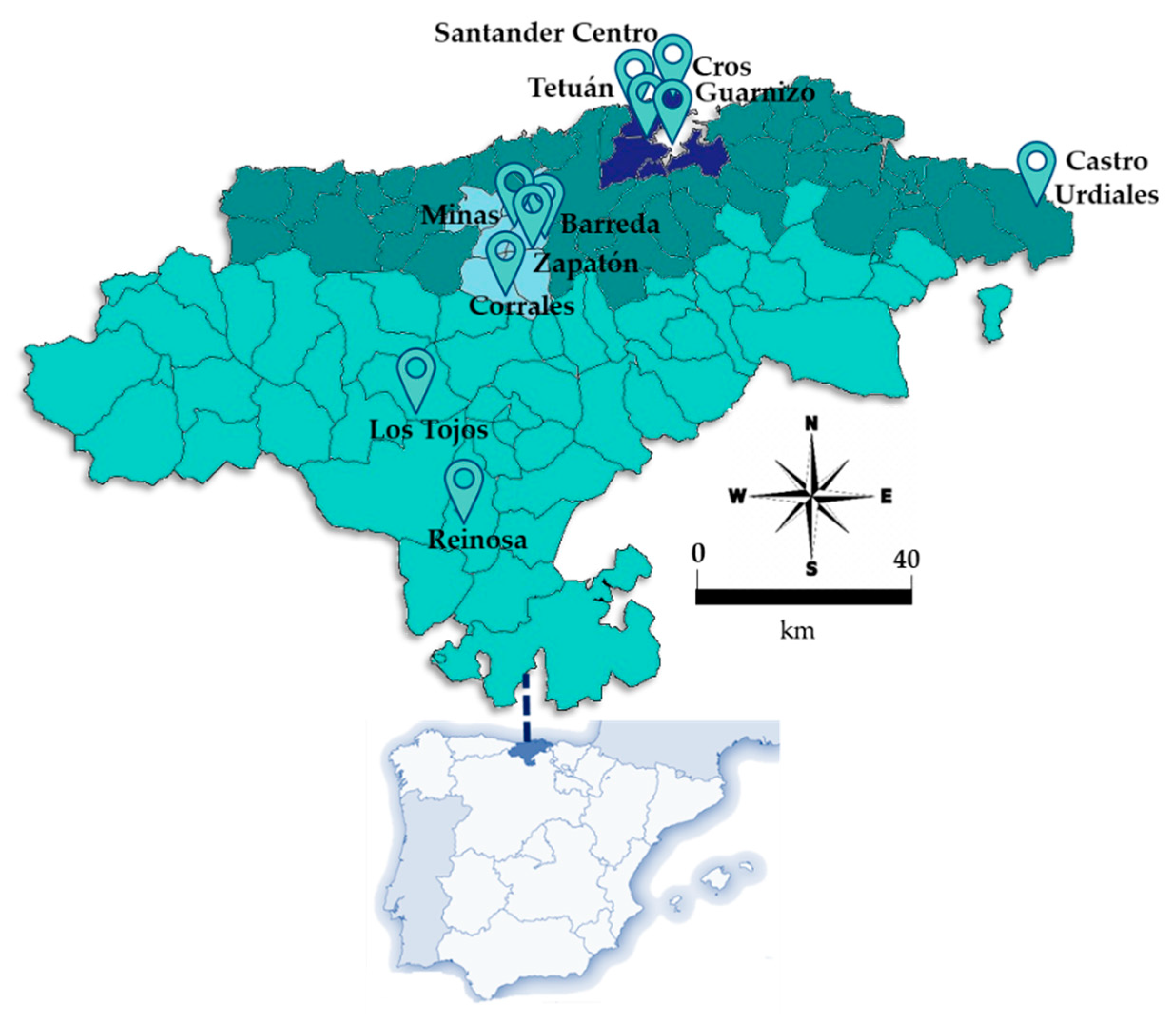
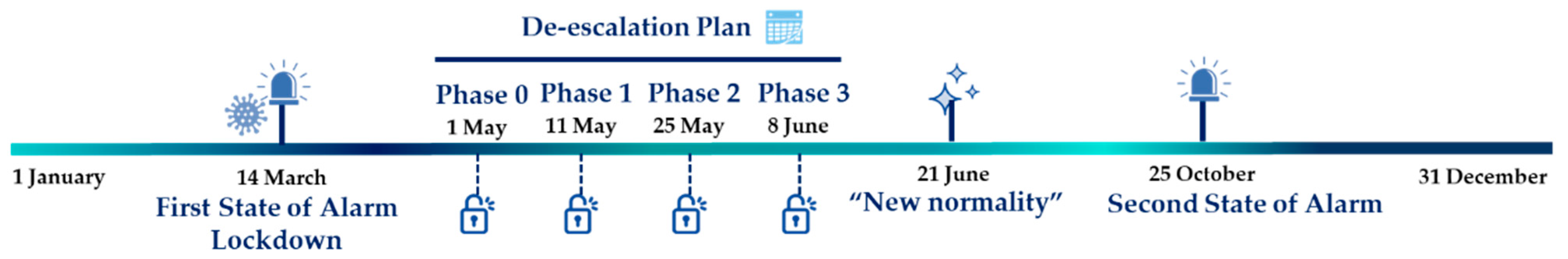
2.1. Area and Period of Study

The study focused on the region of Cantabria, in Northern Spain. The spatial distribution of the population living in this region, constituted by 102 municipalities, is not homogeneous, with 30% of the total inhabitants residing in the city of Santander [57]. The industrial activity is mainly concentrated in two areas: Santander and Torrelavega. Therefore, these cities usually have higher air pollution levels [58]. Despite being a small region (5321 km²), the air quality-monitoring network of Cantabria is formed by 11 stations (Figure 1) of all types: traffic, urban background, industrial and rural. This offered the chance to evaluate the impact of COVID-19 restrictions across all the environments.

To estimate the effect of the crisis during the lockdown, and the subsequent stages, the study covered the full year 2020, divided as follows (Figure 2): (i) Pre-lockdown (1 January–13 March), (ii) Lockdown (First State of alarm) (14 March–30 April), (iii) Phase 0 (1–10 May), (iv) Phase 1 (11–24 May), (v) Phase 2 (25 May–7 June), (vi) Phase 3 (8–20 June), (vii) “New normality” (21 June–24 October), and finally (viii) Second State of Alarm (25 October–31 December).

2.2. Air Quality and Meteorological Data

Air quality data for four key pollutants (NO, NO₂, PM₁₀ and O₃) with 1 h resolution from 2013 to 2020 were retrieved from the European Air Quality Portal [59] using the “saqgetr” R package [60,61], freely available from the CRAN repository (https://cran.r-project.org/, accessed on 1 February 2021). In addition, to check for errors and missing periods of data, pollutant concentration data were also collected from the regional Air Quality Monitoring Network, managed by the Environmental Research Centre of Cantabria [62], which is integrated by 11 fixed stations throughout the territory, as Figure 2 illustrates.

Table 1. Names, codes, type and monitored parameters of the air quality monitoring sites used in the study.

Site	Code	Type	NO2	NO	PM10	O3	Meteorology *
Castro Urdiales	es1578a	Urban background	✔	✔	✔	✔	✔
Corrales	es1579a	Industrial	✔	✔	✔	✔	✔
Guarnizo	es1576a	Industrial	✔	✔	✔	✔	✔
Cros	es1577a	Industrial	✔	✔	✔	✔	✘
Reinosa	es1530a	Urban background	✔	✔	✔	✔	✔
Santander Centro	es1580a	Traffic	✔	✔	✔	✘	✘
Tetuán	es1529a	Urban background	✔	✔	✔	✔	✘
Zapatón	es1038a	Urban background	✔	✔	✔	✔	✘
Barreda	es1037a	Traffic	✔	✔	✔	✘	✘
Minas	es1039a	Traffic	✔	✔	✔	✘	✘
Los Tojos	es1531a	Rural	✔	✔	✔	✔	✔

* Meteorological data for sites that do not have their own meteorological station were obtained from the Spanish Meteorological Agency station at the Santander–Parayas airport.

shows the names, identification codes and classification of the sites into traffic, industrial, urban background and rural; the pollutants monitored at each site are also indicated. A database composed of all station types was employed to study the impact of restrictions in all environments and to draw more specific conclusions that may be useful for the development of future air policies. The selection of these pollutants was based on those with the highest levels, closest to the regulations. Missing data did not represent more than 5% at any site for the total span and were therefore ignored, as they would not affect the overall results due to the huge amount of data used in this study.

Meteorological data were obtained from surface measurements at the air quality monitoring stations specified in Table 1. For the remaining sites that did not cover these parameters, meteorological data were downloaded from the National Oceanic and Atmospheric Administration’s (NOAA) global Integrated Surface Database (ISD) using the R package “worldmet” [63], which is also freely available from the CRAN repository. From this source, data were acquired from the Spanish Meteorological Agency station located at Santander–Parayas airport [64]. An hourly meteorological database including wind speed (ws) [m/s], wind direction (wd) [°], temperature (air-temp) [°C], relative humidity (RH) [%], solar radiation (SR) [W/m²], cloud cover (cl) [oktas], and precipitation (LL) [L/m²] was completed with a 90% or above data capture on each parameter, although not all the variables were available at all the sites. The selection of these variables was based on those most closely related to significant changes in pollutant concentrations [43]. Besides, previous work that aimed to predict hourly concentrations of pollutants showed that models based on more readily accessible meteorological surface measurements were favourable relative to those that used more sophisticated input data (e.g., atmospheric stability and planetary boundary layer), and produced results with higher explanatory power [40].

2.3. Model Development

The weather normalisation procedure to remove meteorological variation from air quality data was conducted using the “deweather” R package [56]. It is part of the “Openair” suite of packages designed to carry out air quality and related data analysis [65]. The fundamentals of the “deweather” package are as follows: it uses a two-step procedure to normalise air quality data. First, models based on the BRT approach for daily concentration of selected air pollutants from different predictors are fitted using the “gbm” package [66]. Then, a meteorological averaging procedure is applied by predicting many times with a random sampling of weather conditions [43,56], using the “metSim” function.

BRTs combine regression trees (i.e., models that relate a response to its predictors) and boosting, an iterative method for developing a final model, progressively adding trees, while re-weighting data to emphasise cases poorly predicted by previous trees [67]. Regression trees model the independent variable Y by means of stratifying or segmenting the predictor space X into a number of simple regions. This involves recursive binary splits of each predictor X_j (different predictors X_1, …, X_p can be considered), at the cutpoint s such that splitting the predictor space into the regions R₁ (j,s) = {X|X_j < s} and R₂ (j,s) = {X|X_j ≥ s} leads to the greatest possible reduction in the residual sum of squares, minimizing Equation (1):

$${\displaystyle \sum }_{i: x_i\in R_1\left(j,s\right)}{\left(y_i-{\widehat{y}}_{R_1}\right)}^2+{\displaystyle \sum }_{i: x_i\in R_2\left(j,s\right)}{\left(y_i-{\widehat{y}}_{R_2}\right)}^2$$

(1)

where ${\widehat{y}}_{R_1}$ is the mean response for the training observation in R₁ (j,s), and ${\widehat{y}}_{R_2}$ is the mean response for the training observations in R₂ (j,s).

The final boosted model $\widehat{f}$ is obtained as a combination of a large number of regression trees f^b (Equation (2)):

$$\widehat{f}\left(x\right)={\displaystyle \sum }_{b=1}^{ntree}\lambda {\widehat{f}}^b\left(x\right)$$

(2)

where λ is the shrinkage or learning rate parameter. Each regression tree f^b is fitted with d splits (interaction depth) to the training data (X, r_i) updating the residuals r_i on each iteration (Equation (3)) [68]:

$$r_i\leftarrow r_i-\lambda {\widehat{f}}^b\left(x_i\right)$$

(3)

In more detail, statistical models were developed using the “gbm” package to explain concentrations based on the meteorological variables cited in the previous section, and temporal variables to forecast the variability linked to the hour of the day, the day of the week and the week of the year. The latter accounted for seasonal meteorological effects not considered by the other parameters. Moreover, the algorithm included a trend term to capture longer-term changes in emission patterns over the period of seven years considered. For each site, the hourly meteorological and pollutant measurements recorded across the total period were randomly divided (by default) into a fraction to train the BRT models (80%) and a fraction for testing its performance (20%), with the aim of developing the most appropriate model. This decision is made automatically with the evaluation of common metrics such as Pearson´s correlation coefficient (r), root mean square error (RMSE) and mean bias (MB). In this study, individual models were built for each pollutant and period of analysis, i.e., 2020 and the reference period (2013–2019). The model fitting parameters were kept as defaults (learning rate = 0.1 and interaction depth = 6.0) as these values were previously optimised using 10-fold cross validation (CV) by other authors [43]. The interaction depth accounts for the interaction between variables. Different number of trees (n.trees) were tested and finally a value of 1000 was used as a compromise between computational time and model performance.

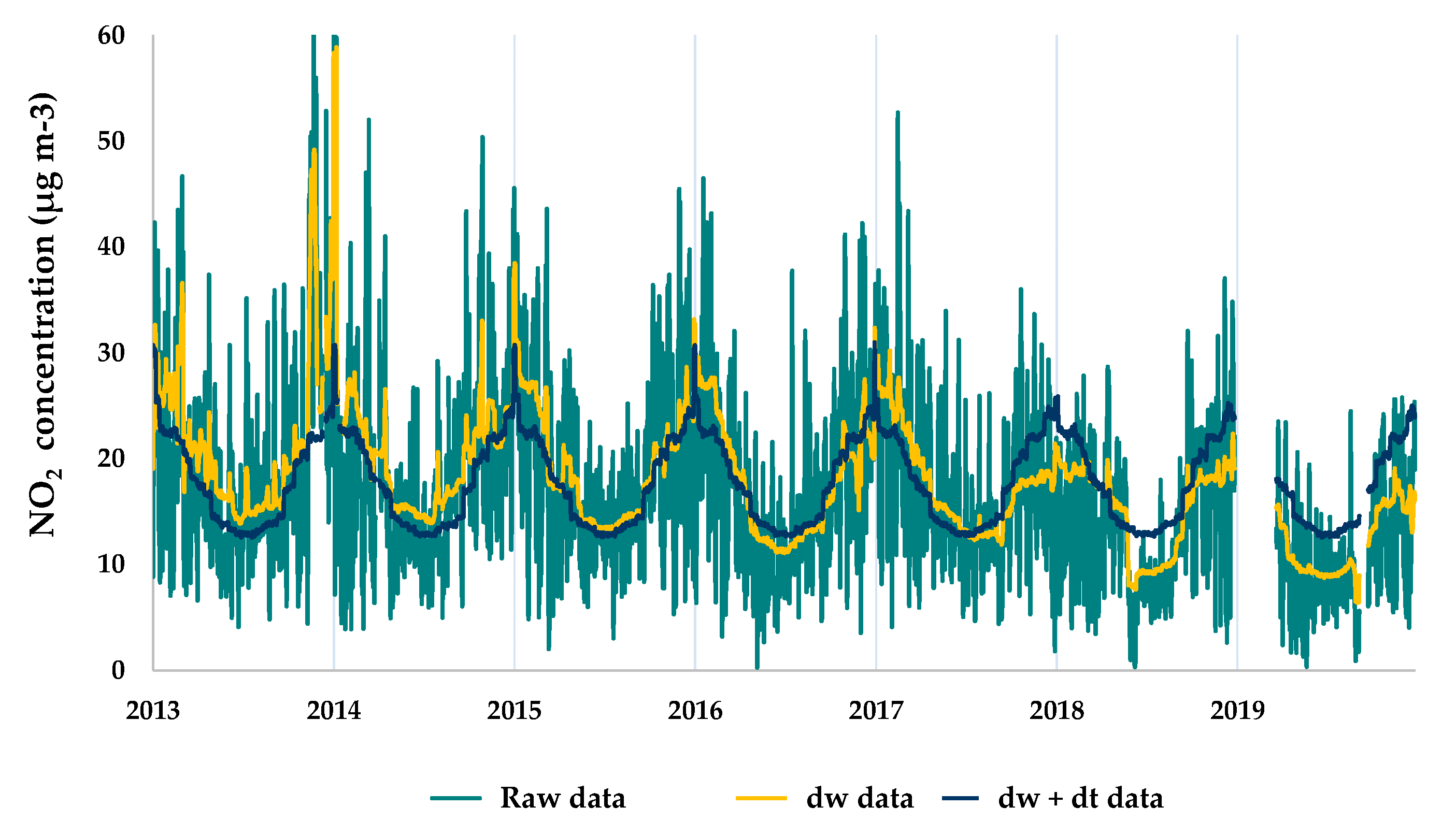
2.3.1. Meteorological Normalisation

Once the model was built, the meteorological averaging procedure was applied by predicting many times with random sampling of weather conditions [56]. This sampling was carried out by the “metSim” function. It is important to note that the model was not used to predict the counterfactual or business as usual (BAU) 2020 scenario, but to predict 2020 concentrations taking into account the drop caused by COVID-19, and removing the meteorological variability. In practice, new time series of concentrations are generated for random samples of meteorology hundreds of times. This approach yields a single, new time series of predicted concentrations that represents average meteorology. An example of the deweathered (dw) time series for 2020 is shown in Figure 3.

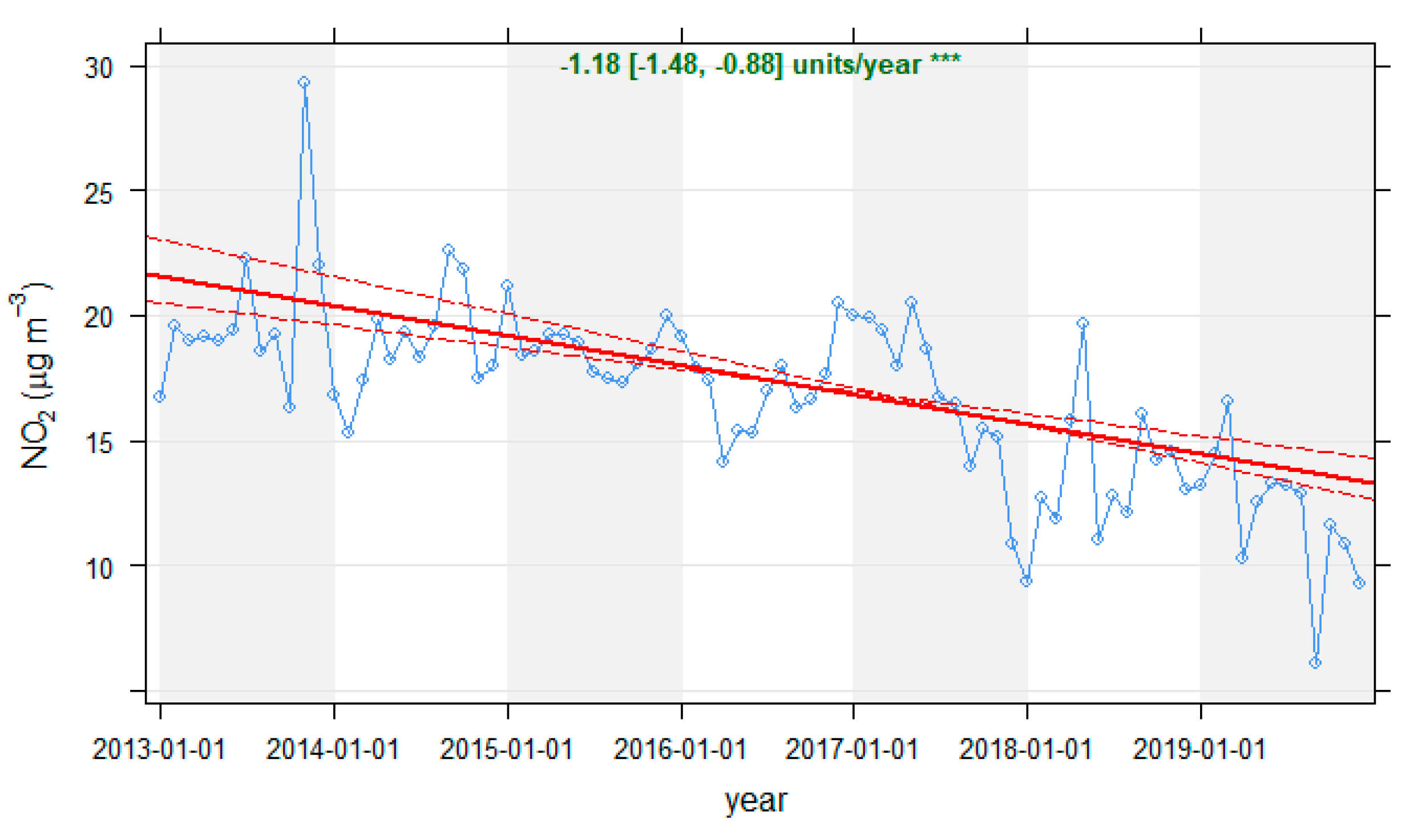
2.3.2. Emission Pattern Trends Normalisation

Data concentrations of the reference period (2013–2019) were analysed using the “TheilSen” function implemented in “Openair”, to characterise general air quality trends prior to lockdown. The method provided a non-parametric measurement of trends on “a median of slopes of pairs of points with different x-values” estimation of the slope (Figure 4), and bootstrap estimation of uncertainty [69]. These trends from previous years may mask the results, leading to erroneous conclusions, so a similar procedure to weather normalisation was employed to remove them. By including the “trend” term in the “metSim” function, emission trends were averaged, so the reference period converted into a fixed emissions scenario [43]. An example of the detrended (dt) time series is shown in Figure 5.

It is important to highlight that, because the study made a daily comparison, i.e., each day of the year 2020 was compared with the same day of the average (2013–2019), the variable “week” was not normalised, as this variable represented the seasonal changes attributed to each week of the year, which were observed in both data series. By contrast, the day of the week was normalised, because weekly patterns of pollutant concentrations are important, mainly due to differences between working days and weekends [70].

2.4. Quantification of Changes

Equation (4) was applied to raw (unnormalised) data to calculate the observed changes in air pollutant levels. The percentage of change (P) in each period (i) was obtained individually for each air pollutant at each site as follows:

$$P(\%)periodi=\frac{\overline{C_{2020,periodi}}-\overline{C_{2013-2019,periodi}}}{\overline{C_{2020,period\mathrm{i}}}}\times 100$$

(4)

where $\overline{C_{2020,period i}}$ corresponds to the average concentration of a given pollutant at a given station, in each period i of the year 2020: pre-lockdown, lockdown, phase 0, phase 1, phase 2, phase 3, “new normality” and 2nd State of Alarm; and $\overline{C_{2013-2019,period i}}$ represents the mean concentration of the same pollutant in the same period, averaged over the last seven years.

In order to further obtain the normalised percentage changes (P_dwdt) (after removing meteorological and emission trend influences), a similar process using Equation (5) was followed:

$$P_{dwdt}(\%) period i=\frac{\overline{C_{\left(2020\right)dw,period i}}-\overline{C_{\left(2013-2019\right)dw+dt, period i}}}{\overline{C_{\left(2020\right)dw,period i}}} \times 100$$

(5)

As explained in Section 2.3, the “deweather” procedure was applied to the complete database, whereas the “detrend” procedure was only implemented for (2013–2019) data; thus, the terms in Equation (2) were $\overline{C_{\left(2020\right)dw,period i}}$ and $\overline{C_{\left(2013-2019\right)dw+dt,period i}}$, respectively.

3. Results and Discussion

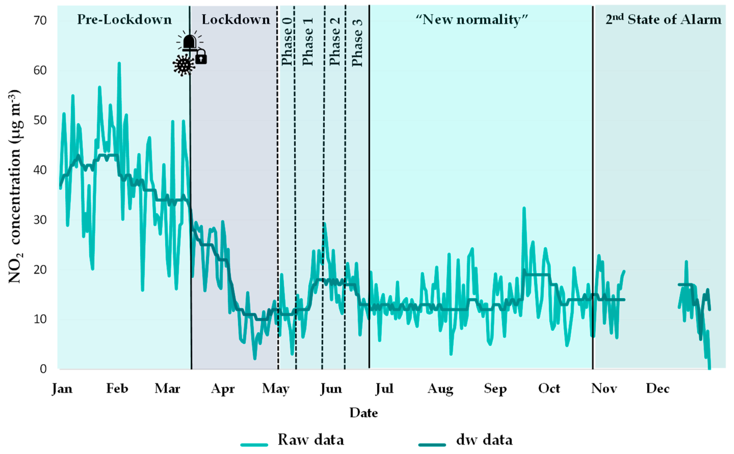
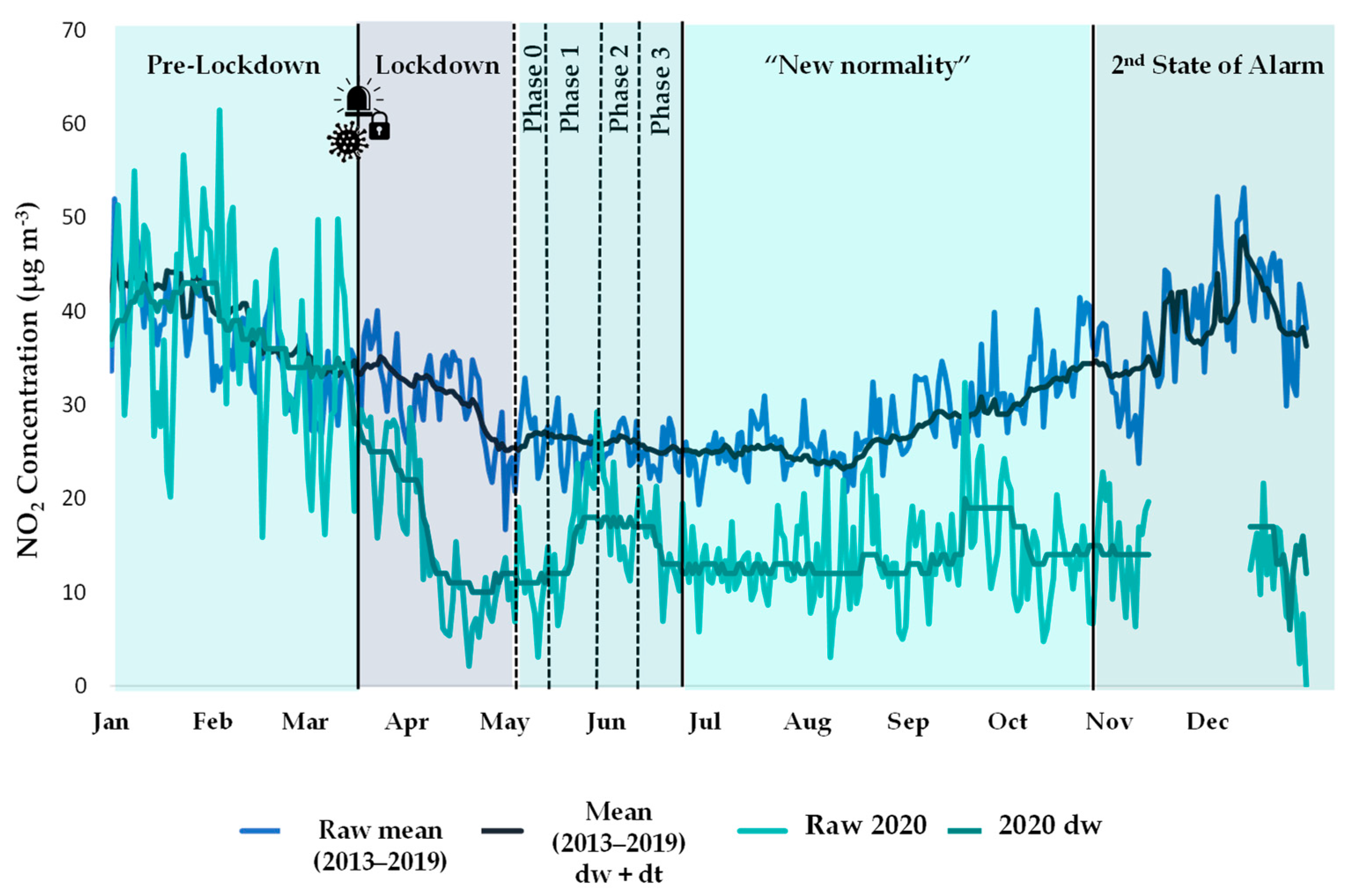
3.1. Observed Changes

Figure 6 (light blue and green series) presents the observed daily NO₂ concentrations for the full year 2020 at Santander Centro (except for a short period in December when no data were available) divided into periods according to COVID-19 restrictions and compared with the mean levels recorded in the previous seven years. During the lockdown, concentrations registered a significant drop. In the following periods of de-escalation, with the relaxation of some limitations, levels increased but remained far below the previous years. Finally, during the Second State of Alarm, which was much less stringent than the first in terms of mobility, NO₂ concentrations remained more than halved at this location. This comparison was obtained for each pollutant at each site, but to condense the results, they were grouped and summarised in a box plot (Figure 7, series in blue). Nevertheless, in some cases the pollutant concentrations at a specific site, such as PM₁₀ at Los Tojos, are not included in the chart because of some anomalies that would have distorted the results.

Figure 7 depicts that mean pre-lockdown levels were lower than the baseline period for pollutants such as NO₂ and O₃, whose concentrations in 2020 were around −23% in both cases, whereas for NO and PM₁₀ the year started with higher levels, +10% and +34%, respectively. These changes varied greatly between sites, suggesting that different emission and meteorological patterns occurred in early 2020 (i.e., before the lockdown) with respect to the reference period. Querol et al. [71] analysed the meteorological patterns during the pre-pandemic period in Spain, comparing it with the previous years (2015–2019), and found weather anomalies that induced higher than usual wind speeds, temperature increases, lower precipitation, and cloudiness over the Bay of Biscay, which is close to the region studied here. Under that scenario, they reported gains in PM₁₀ levels in pre-lockdown in Bilbao that ranged from +1% (at urban background sites) to +23% (at traffic sites). The cited values were obtained after the subtraction of African dust outbreaks which were abundant in the north of the peninsula during the pre-lockdown and the early days of the lockdown, as reported by the Ministry for the Ecological Transition and the Demographic challenge [72]; thus, they seem to be in line with our findings (from raw data without removing dust intrusions). They also quantified an average reduction of −22% in NO₂ and −8% in O₃, the latter being significantly lower than our results, although the comparison is not straightforward as they used 8 h measurements whereas we used daily averaged concentrations.

The lockdown of 14 March led to significant decreases in nitrogen oxide concentrations, −65% for NO₂ and −57% for NO (average of the sites considered) (see Figure 7), as a result of a drastic reduction in traffic, of up to −90% in some Spanish cities [73]. These results are comparable to the observations of Tobías et al. [6] and Baldasano [74] for traffic sites in Barcelona (−51%) and in Madrid (−62%) [18]; Querol et al. [71] published, as an average, −51% for eleven cities in Spain considering several site types; and Ordóñez et al. [75] observed at urban sites a decrease of −51.6% in Spain. These findings also confirmed the general trend found worldwide by the experts [11,19,33,75,76,77,78,79], including Spain among the three most affected European countries with the highest NO₂ reductions. However, the measured average reduction in PM₁₀ was below −5% and O₃ decreased by −10%. These percentages express the variation with respect to the baseline (2013–2019), but considering the changes in lockdown versus the pre-lockdown period, the outcomes are somewhat different for some pollutants.

Taking average PM₁₀ reductions as an example, when comparing both periods (i.e., before and during lockdown) it was observed that the change went from a positive (+34%) to a negative gain (−5%). Thus, the decrease was substantial, but perhaps not directly induced by the COVID-19 restrictions because the variation with respect to the baseline scenario was minimal. This highlights the relevance of choosing a robust comparison period. Many papers showed large reductions in air pollution levels, but if they simply compare the levels in lockdown with the previous months, they do not account for seasonality, which is crucial when studying air pollution trends, as emphasised during the introduction. Globally, the impact of COVID-19 on PM₁₀ levels ranged from −9 to −60%, according to a recent review carried out by Marinello et al. [17]. Querol et al. [71] obtained lockdown changes in PM₁₀ that varied significantly from one Spanish city to another, and between the different site types studied. Lovrić et al. [49] also claimed reductions in PM₁₀ that were not as pronounced as in NO₂ in the Austrian city of Graz. As they explained, that fact demonstrated that traffic is just one of many contributing sources to PM₁₀. Thus, some natural sources of PM₁₀, such as marine aerosol, crustal material including Saharan intrusions, and some secondary inorganic aerosols not directly related to road traffic (ammonium sulphate) may notably contribute to the levels of PM₁₀ measured in some of these studies, as reported in a former study carried out in the Cantabria region [80].

With respect to O₃, it is necessary to point out that the observed variation during lockdown, −10% on average below the baseline at the region studied, did not follow the general trend recorded across Europe by authors such as Grange et al. [55], where mean O₃ concentrations increased by a similar magnitude to the decrease in NO₂. In fact, they reported an increase in O₃ levels in Spain of between +37 and +61%, comparing the observed values with those estimated in the BAU scenario. This O₃ increment linked to the lockdown was also found in Spain by Gorrochategui et al. [81] and Tobías et al. [6]. However, although Ordóñez et al. [75] reported O₃ increases over most of Europe, both at urban background and rural sites, an average raw reduction of −10% was found in Spain.

However, it is necessary to highlight that important differences between sites were registered in the Cantabrian network, with positive relative changes in O₃ concentrations at Tetuán (Santander urban background) and Cros (industrial) sites, indicating the importance of local sources of different precursors on O₃ formation. In this line, Querol et al. [70] described different responses of urban O₃ but a generalized and light decrease in rural locations. Therefore, this needs to be further investigated, bearing in mind the complex behaviour of O₃ during the lockdown, which can be partially explained by the alteration of the photolytic cycle due to a strong decrease in NO levels in a VOCs-limited environment (usually urban areas) [82], which acts on the consumption of O₃ in the titration reaction (NO + O₃ ↔ NO₂ + O₂) [49,83]_. However, the different intensities of reductions in emissions of other O₃ precursors, such as NMVOCs, may have led to different levels of tropospheric O₃ in different regions, according to the results found by other authors [84,85]. In addition, considerable O₃ production downwind of sources only happens during periods of sustained insolation and high temperatures. Hence, the role of meteorology also needs to be examined [35,75].

During the de-escalation phases, NO and NO₂ followed a similar pattern, gradually increasing concentrations with the reduction of restrictions, but keeping far away from the reference scenario. PM₁₀ and O₃ showed a more complex trend (see Figure 7), not easily related to the progressive lifting of COVID-19 limitations. Finally, with the Second State of Alarm, there were some falls, but generally of smaller magnitudes than in March (−48% NO₂).

Nonetheless, as our findings have so far only been derived from the raw data, we will discuss them in detail if, after disentangling meteorological and trend influences from the observed data, there are substantial modifications.

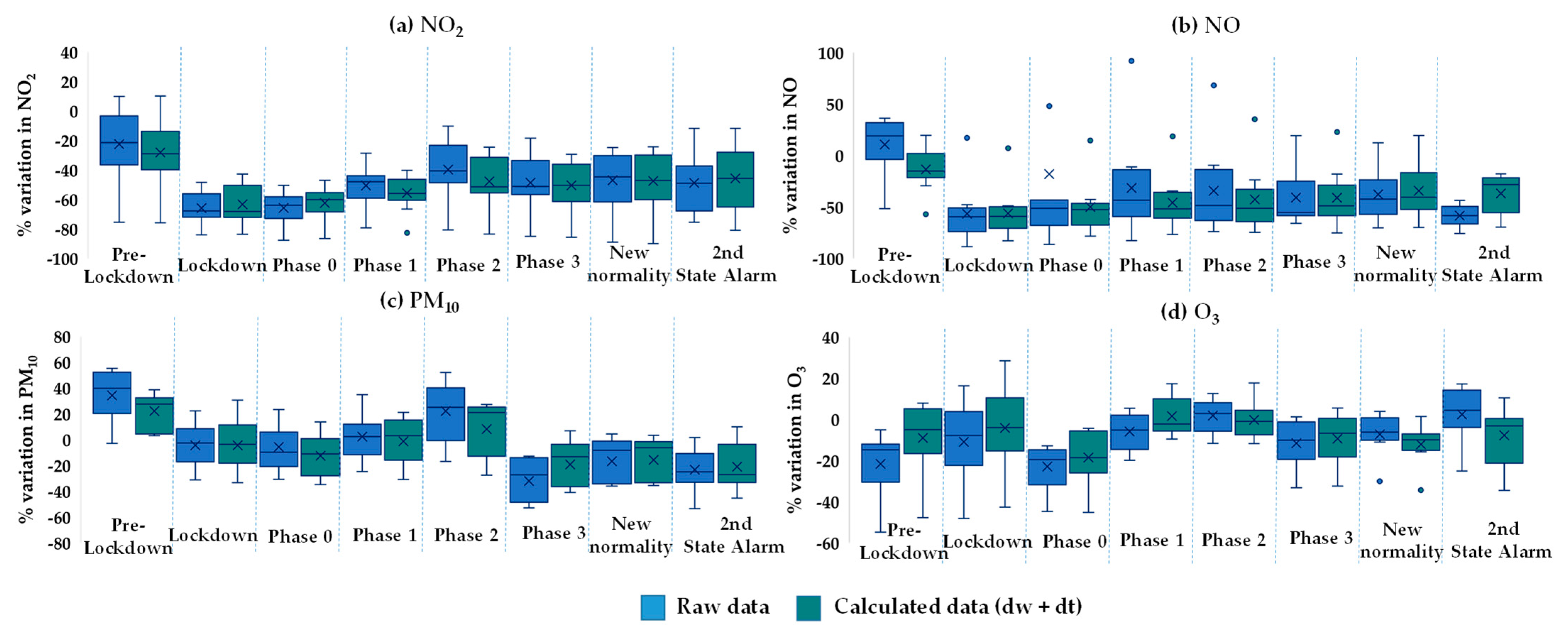
3.2. Estimated Changes

The estimated results obtained using the BRT models of the “deweather” package are presented and discussed in this section. Figure 6 shows an example of the application to NO₂ at the Santander Centro site of the meteorological normalisation described in Section 2.3.1 and the emission pattern trends normalisation explained in Section 2.3.2. As can be seen in the example, the model removed the noise in the graph, which probably corresponded to daily concentration peaks resulting from extreme values of some meteorological predictors; therefore, this procedure makes it easier to clearly observe the response to COVID-19 lockdown on pollutant concentrations. Thus, the percentage change was the gap between the darkest lines (see Figure 6). Again, this comparison was obtained for each pollutant at each site, and the results were summarised and compared with the observed ones in the box plot shown above in Figure 7 (series in green).

From this figure, pollutant concentration changes over the calendar year both from deweathered/detrended and raw data generally demonstrated a similar pattern, although in some cases the magnitude of the change varied slightly, mainly for O₃. Furthermore, in general, the interquartile range of the concentrations underwent a minimisation after the correction because of the subtraction of meteorological variability.

Pre-lockdown could be considered as a validation step in which the model performance could be tested. In an ideal scenario in which the model is able to fully decouple the influences of weather and emission trends, the percentage change (2020 vs. 2013–2019) in pre-lockdown would be virtually null. As can be witnessed in Figure 7, the model improved the gap in the pre-lockdown period, except for NO₂. The best results were found for the cases of PM₁₀ (+20%) and O₃ (−10%), where the average variation moved closer to zero. Nevertheless, the starting point was slightly far from the ideal situation. Petetin et al. [53] also obtained a moderate positive bias before lockdown, in Madrid and Barcelona, using a machine learning model. A possible reason for these biases is the lack of some additional predictors that can improve the performance of the BRT model and then the normalised results. Among these, the atmospheric stability and/or planetary boundary layer height can be a key factor, having a significant influence on pollutant dispersion and accumulation [40]. Mor et al. [85] discussed that the increase in air temperature associated with the onset of summer season had a direct impact on the stability of the atmosphere, decreasing it and thus increasing the mixing height of pollutants, which lead to the increment of the vertical mixing ratio in the troposphere. Despite the relevant importance of this variable, it was also not introduced in the model, as no data were available from the sources used. Apart from these considerations, there are many other potential explanations for anomalies in the data, from failures in the measurement equipment to episodic cases of garbage burning [31], or construction work in the surroundings of a monitoring site. In addition, the contributions of African dust outbreaks to the levels of PM₁₀ were not included among the model predictors.

Furthermore, the model did not fully eliminate the NO outliers (see Figure 7) during de-escalation phases, but it did reduce their magnitude, so it is reasonable to think that they were the result of unusual episodes not only related to meteorological conditions, taking into account that they were all recorded at the same station (Tetuán, urban background).

With respect to the lockdown period, the normalisation procedure did not produce large changes in the calculation of the relative variations for NO, NO₂ and PM₁₀ at most of the sites, as observed in Figure 7. However, the relative change in O₃ is lower than the observed change, becoming positive values at some sites. In contrast, during the second lockdown, O₃ relative changes were larger (more negative) than those observed, probably due to the opposite behaviour of NO (smaller decrease in NO levels than observed).

3.3. Analysis of the Traffic Sites

The impacts of road vehicle reductions during the lockdown were more dramatic in the close proximity of roads in comparison with more distant urban background locations [86], so variations at traffic sites were individually analysed using raw and normalised data.

To visualise the impacts of traffic restrictions on air pollution, Figure 8 depicts the daily patterns of NO, NO₂ and PM₁₀ at roadsides during 2020 lockdown (from 14 March to 1 May) and the equivalent period of the previous seven years (2013–2019). In addition, weekdays, weekends and the non-essential activity shutdown period in Spain (from 30 March to 9 April) were considered separately, as it is well known that weekly patterns have also a relevant importance in emissions [87]. NO and NO₂ levels in the baseline scenario (dashed lines) showed a daily profile characterised by two peaks that are related to rush hours [49], around 8 a.m. and 8 p.m., hours in which arrivals and departures in work environments, educational centres, shopping centres, etc., take place. During rush hours, NO₂ reached the higher levels, of around 50 µg/m³, and NO concentrations were over 15–40 µg/m³ in the morning. By comparison, the NO second peak was smaller (5–15 µg/m³). Looking at Figure 8 it can be clearly confirmed that the lockdown had a major impact on traffic and thus on the levels of traffic-sourced pollutants (solid lines). The typical 8 a.m. peak diminished markedly as NO₂ and NO did not exceed 30 and 10 µg/m³, respectively, and the afternoon peak almost completely disappeared. Regarding the PM₁₀ levels, the daily pattern was not as clear, but a drop during lockdown was also observed at some sites, whereas at others there was even a little increase. The differences between working days and weekends were not as remarkable and the cessation of non-essential activity either meant big differences in comparison with the rest of lockdown period.

Globally, when traffic stations were analysed separately, they exhibited a raw reduction in NO₂ during lockdown with a median value of −56%, which moved to −45% after the correction (see

Table 2. Change (%) in pollutant concentrations at traffic sites for each period in the region under study, using raw and normalised data (dwdt).

Site/Pollutant		Pre-Lockdown		Lockdown		Phase 0		Phase 1		Phase 2		Phase 3		New Normality		2nd State of Alarm
		Raw	dwdt	Raw	dwdt	Raw	dwdt	Raw	dwdt	Raw	dwdt	Raw	dwdt	Raw	dwdt	Raw	dwdt
Santander	NO2	+3.2	−2.3	−48.4	−42.8	−60.4	−55.8	−45.8	−51.5	−23.7	−32.4	−35.8	−37.7	−50.4	−49.6	−66.8	−62.1
	NO	+13.6	−18.8	−59.1	−62.1	−43.4	−48.1	−38.4	−46.3	−73.9	−63.8	−58.0	−56.8	−44.8	−40.9	−64.3	−62.3
	PM10	+52.1	+38.6	−2.7	−2.2	+4.0	−5.3	+11.5	+5.8	+44.6	+21.9	−15.1	−2.3	+4.3	−0.3	−10.9	−1.6
Barreda	NO2	+9.9	+10.1	−56.1	−45.3	−50.4	−58.8	−58.7	−58.5	−43.1	−52.1	−44.3	−49.1	−46.8	−49.5	−49.5	−48.4
	NO	+29.2	+1.5	−77.0	−69.6	−51.0	−58.3	−42.5	−52.3	−28.1	−42.0	−18.9	−36.7	−27.3	−27.5	−47.1	−38.7
	PM10	−2.9	+3.0	−31.2	−33.4	−30.7	−34.9	−24.7	−30.9	−16.9	−27.5	−49.4	−41.0	−29.9	−30.5	−33.1	−28.0
Minas	NO2	−14.9	−20.3	−68.8	−69.8	−71.9	−67.7	−45.8	−55.5	−44.9	−52.1	−51.5	−51.8	−42.5	−44.7	−48.0	−30.4
	NO	+11.7	−4.6	−72.9	−72.6	−76.9	−67.4	−54.1	−59.2	−55.5	−52.0	−57.0	−48.0	−44.6	−40.8	−62.3	−29.9
	PM10	+20.6	+14.2	−12.8	−18.2	−21.7	−28.0	−15.2	−19.8	−0.7	−12.9	−47.0	−38.2	−35.4	−35.6	−31.7	−27.0
Median	NO2	+3.2	−2.3	−56.1	−45.3	−60.4	−58.8	−45.8	−55.5	−43.1	−52.1	−44.3	−49.1	−46.8	−49.5	−49.5	−48.4
	NO	+13.6	−4.6	−72.9	−69.6	−51.0	−58.3	−42.5	−52.3	−55.5	−52.0	−57.0	−48.0	−44.6	−40.8	−62.3	−38.7
	PM10	+20.6	+14.2	−12.8	−18.2	−21.7	−28.0	−15.2	−19.8	−0.7	−12.9	−47.0	−38.2	−29.9	−30.5	−31.7	−27.0

). These reductions in NO₂ concentrations at traffic sites, where road traffic is virtually the only source of this pollutant, were only slightly lower than those found for the region on average, suggesting that most of the total reduction found in the region is due to road traffic, with the contribution from industry and other sources being much smaller. For NO and PM₁₀, the correction meant less changes, from a reduction of −73 to −70% and from −13 to −18%, respectively.

In relation to the pre-lockdown, the so-called “validation phase”, the median of the estimated values at traffic sites was closer to zero than considering the total sites, reaching −2% for NO₂, −5% for NO and +14% for PM_10. These percentages may indicate that the model performed better for the traffic stations, as there is only one main source of pollution there, which can be more easily described, despite not including a predictor variable that accounts for direct vehicle emissions.

Table 2 also shows that the situation after lockdown varied moderately, and it is difficult to state general trends, but overall pollutant levels at traffic sites remained lower than the baseline before and after the normalisation procedure.

4. Conclusions

The COVID-19 pandemic and the unprecedented measures adopted during this emergency situation produced side effects on air quality levels due to the large reduction in anthropogenic emissions. This study analysed these effects on air pollutant levels using raw and normalised data series (2013–2020) from a Northern Spanish region (Cantabria), by means of the “deweather” R package, which was used to decouple meteorological and patterns in emission trends from the observed data.

The main outcomes revealed that lockdown restrictions resulted in large reductions in nitrogen oxides, −65% for NO₂ and −57% for NO; and moderate decreases in PM₁₀ (−5%) and O₃ (−10%). The trend observed for NO_x was consistent with strong traffic reductions, as stated in the recent literature. However, the outcomes for PM₁₀ and O₃ were highly variables from study to study, highlighting their complex behaviour and making it difficult to observe general trends. By comparison, the normalised results (“deweathered” and “detrended”) showed relative variations for the studied pollutants in line with observations, exhibiting a general reduction in variability. In addition, the pre-lockdown period revealed anomalous lower observed levels than the reference period for NO₂ and O₃ (−23%) and higher levels for NO and PM₁₀ (+10 and +34%, respectively); these gaps improved after data normalisation, except for NO₂, but still were far from zero, evidencing the lack of some additional model predictors.

The results demonstrated air quality improvement, mostly related to traffic reductions, so it is imperative to take measures to boost the transition to sustainable mobility by means of the creation of traffic reduction policies (e.g., implementation of Low Emission Zones (LEZs) and electrification of the vehicle fleet). As a longer-term strategy, authorities are advised to develop an effective integrated policy to reduce emissions from other sectors by replacing fossil fuels with sustainable alternatives, and by raising public concern on environmental issues, as the health of the population is at stake.

References

1. Lu, R.; Zhao, X.; Li, J.; Niu, P.; Yang, B.; Wu, H.; Wang, W.; Song, H.; Huang, B.; Zhu, N.; et al. Genomic characterisation and epidemiology of 2019 novel coronavirus: Implications for virus origins and receptor binding. Lancet 2020, 395, 565–574. [Google Scholar] [CrossRef] [Green Version]
2. Nicola, M.; Alsafi, Z.; Sohrabi, C.; Kerwan, A.; Al-Jabir, A.; Iosifidis, C.; Agha, M.; Agha, R. The socio-economic implications of the coronavirus pandemic (COVID-19): A review. Int. J. Surg. 2020, 78, 185–193. [Google Scholar] [CrossRef]
3. WHO. Coronavirus Disease (COVID-19) Pandemic. Available online: https://www.who.int/emergencies/diseases/novel-coronavirus-2019 (accessed on 5 July 2021).
4. ISCIII. Situación del COVID-19 en España. Available online: https://cnecovid.isciii.es/covid19/ (accessed on 1 July 2021).
5. España. Real Decreto 463/2020, de 14 de marzo, por el que se declara el estado de alarma para la gestión de la situación de crisis sanitaria ocasionada por el COVID-19. Boletín Oficial del Estado; núm. 67. Available online: https://www.boe.es/eli/es/rd/2020/03/14/463/con (accessed on 22 April 2021).
6. Tobías, A.; Carnerero, C.; Reche, C.; Massagué, J.; Via, M.; Minguillón, M.C.; Alastuey, A.; Querol, X. Changes in air quality during the lockdown in Barcelona (Spain) one month into the SARS-CoV-2 epidemic. Sci. Total Environ. 2020, 726, 138540. [Google Scholar] [CrossRef] [PubMed]
7. Martorell-Marugán, J.; Villatoro-García, J.A.; García-Moreno, A.; López-Domínguez, R.; Requena, F.; Merelo, J.J.; Lacasaña, M.; de Dios Luna, J.; Díaz-Mochón, J.J.; Lorente, J.A.; et al. DatAC: A visual analytics platform to explore climate and air quality indicators associated with the COVID-19 pandemic in Spain. Sci. Total Environ. 2021, 750, 141424. [Google Scholar] [CrossRef] [PubMed]
8. Gobierno de España, Ministerio de Sanidad. Plan Para la Transición Hacia Una Nueva Normalidad. 2020. Available online: https://www.lamoncloa.gob.es/lang/en/gobierno/councilministers/paginas/2020/20200428council.aspx (accessed on 6 December 2021).
9. CNE. COVID-19 en España. Available online: https://cnecovid.isciii.es/ (accessed on 3 July 2021).
10. España. Real Decreto 926/2020, de 25 de Octubre, Por El Que Se Declara El Estado de Alarma Para Contener La Propagación de Infecciones Causadas Por el SARS- CoV-2. Boletín Oficial del Estado; núm. 282. Available online: https://www.boe.es/eli/es/rd/2020/10/25/926 (accessed on 24 April 2021).
11. Muhammad, S.; Long, X.; Salman, M. COVID-19 pandemic and environmental pollution: A blessing in disguise? Sci. Total Environ. 2020, 728, 138820. [Google Scholar] [CrossRef] [PubMed]
12. Viteri, G.; Díaz de Mera, Y.; Rodríguez, A.; Rodríguez, D.; Tajuelo, M.; Escalona, A.; Aranda, A. Impact of SARS-CoV-2 lockdown and de-escalation on air-quality parameters. Chemosphere 2021, 265, 129027. [Google Scholar] [CrossRef]
13. Le, T.; Wang, Y.; Liu, L.; Yang, J.; Yung, Y.L.; Li, G.; Seinfeld, J.H. Unexpected air pollution with marked emission reductions during the COVID-19 outbreak in China. Science 2020, 369, 702–706. [Google Scholar] [CrossRef] [PubMed]
14. Mesas-Carrascosa, F.J.; Porras, F.P.; Triviño-Tarradas, P.; García-Ferrer, A.; Meroño-Larriva, J.E. Effect of lockdown measures on atmospheric nitrogen dioxide during SARS-CoV-2 in Spain. Remote Sens. 2020, 12, 2210. [Google Scholar] [CrossRef]
15. Zhang, Z.; Arshad, A.; Zhang, C.; Hussain, S.; Li, W. Unprecedented temporary reduction in global air pollution associated with COVID-19 forced confinement: A continental and city scale analysis. Remote Sens. 2020, 12, 2420. [Google Scholar] [CrossRef]
16. Shi, Z.; Song, C.; Liu, B.; Lu, G.; Xu, J.; Van Vu, T.; Elliott, R.J.R.; Li, W.; Bloss, W.J.; Harrison, R.M. Abrupt but smaller than expected changes in surface air quality attributable to COVID-19 lockdowns. Sci. Adv. 2021, 7, eabd6696. [Google Scholar] [CrossRef]
17. Marinello, S.; Butturi, M.A.; Gamberini, R. How changes in human activities during the lockdown impacted air quality parameters: A review. Environ. Prog. Sustain. Energy 2021, 40, 1–18. [Google Scholar] [CrossRef] [PubMed]
18. Gkatzelis, G.I.; Gilman, J.B.; Brown, S.S.; Eskes, H.; Gomes, A.R.; Lange, A.C.; McDonald, B.C.; Peischl, J.; Petzold, A.; Thompson, C.R.; et al. The global impacts of COVID-19 lockdowns on urban air pollution: A critical review and recommendations. Elem. Sci. Anthr. 2021, 9. [Google Scholar] [CrossRef]
19. Bauwens, M.; Compernolle, S.; Stavrakou, T.; Müller, J.F.; van Gent, J.; Eskes, H.; Levelt, P.F.; van der A, R.; Veefkind, J.P.; Vlietinck, J.; et al. Impact of Coronavirus Outbreak on NO2 Pollution Assessed Using TROPOMI and OMI Observations. Geophys. Res. Lett. 2020, 47, 1–9. [Google Scholar] [CrossRef] [PubMed]
20. Mendez-Espinosa, J.F.; Rojas, N.Y.; Vargas, J.; Pachón, J.E.; Belalcazar, L.C.; Ramírez, O. Air quality variations in Northern South America during the COVID-19 lockdown. Sci. Total Environ. 2020, 749, 141621. [Google Scholar] [CrossRef]
21. Nakada, L.Y.K.; Urban, R.C. COVID-19 pandemic: Impacts on the air quality during the partial lockdown in São Paulo state, Brazil. Sci. Total Environ. 2020, 730, 139087. [Google Scholar] [CrossRef]
22. Zambrano-Monserrate, M.A.; Ruano, M.A.; Sanchez-Alcalde, L. Indirect effects of COVID-19 on the environment. Sci. Total Environ. 2020, 728, 138813. [Google Scholar] [CrossRef]
23. Ghahremanloo, M.; Lops, Y.; Choi, Y.; Mousavinezhad, S. Impact of the COVID-19 outbreak on air pollution levels in East Asia. Sci. Total Environ. 2021, 754, 142226. [Google Scholar] [CrossRef]
24. Ecologistas en Acción. Efectos de la Crisis de la COVID-19 En La Calidad del Aire Urbano en España. 2020. Available online: https://www.ecologistasenaccion.org/wp-content/uploads/2020/05/informe-3-calidad-aire-covid-19.pdf (accessed on 13 December 2021).
25. Jephcote, C.; Hansell, A.L.; Adams, K.; Gulliver, J. Changes in air quality during COVID-19 ‘lockdown’ in the United Kingdom. Environ. Pollut. 2021, 272, 116011. [Google Scholar] [CrossRef]
26. Venter, Z.S.; Aunan, K.; Chowdhury, S.; Lelieveld, J. COVID-19 lockdowns cause global air pollution declines. Proc. Natl. Acad. Sci. USA 2020, 117, 18984–18990. [Google Scholar] [CrossRef]
27. Domínguez-Amarillo, S.; Fernández-Agüera, J.; Cesteros-García, S.; González-Lezcano, R.A. Bad air can also kill: Residential indoor air quality and pollutant exposure risk during the COVID-19 crisis. Int. J. Environ. Res. Public Health 2020, 17, 7183. [Google Scholar] [CrossRef]
28. Hashim, B.M.; Al-Naseri, S.K.; Al-Maliki, A.; Al-Ansari, N. Impact of COVID-19 lockdown on NO2, O3, PM2.5 and PM10 concentrations and assessing air quality changes in Baghdad, Iraq. Sci. Total Environ. 2021, 754, 141978. [Google Scholar] [CrossRef]
29. Briz-Redón, Á.; Belenguer-Sapiña, C.; Serrano-Aroca, Á. Changes in air pollution during COVID-19 lockdown in Spain: A multi-city study. J. Environ. Sci. 2021, 101, 16–26. [Google Scholar] [CrossRef]
30. Nigam, R.; Pandya, K.; Luis, A.J.; Sengupta, R.; Kotha, M. Positive effects of COVID-19 lockdown on air quality of industrial cities (Ankleshwar and Vapi) of Western India. Sci. Rep. 2021, 11, 1–12. [Google Scholar] [CrossRef] [PubMed]
31. Kerimray, A.; Baimatova, N.; Ibragimova, O.P.; Bukenov, B.; Kenessov, B.; Plotitsyn, P.; Karaca, F. Assessing air quality changes in large cities during COVID-19 lockdowns: The impacts of traffic-free urban conditions in Almaty, Kazakhstan. Sci. Total Environ. 2020, 730, 139179. [Google Scholar] [CrossRef]
32. Zhong, Q.; Ma, J.; Shen, G.; Shen, H.; Zhu, X.; Yun, X.; Meng, W.; Cheng, H.; Liu, J.; Li, B.; et al. Distinguishing Emission-Associated Ambient Air PM2.5 Concentrations and Meteorological Factor-Induced Fluctuations. Environ. Sci. Technol. 2018, 52, 10416–10425. [Google Scholar] [CrossRef] [Green Version]
33. Wang, P.; Chen, K.; Zhu, S.; Wang, P.; Zhang, H. Severe air pollution events not avoided by reduced anthropogenic activities during COVID-19 outbreak. Resour. Conserv. Recycl. 2020, 158, 104814. [Google Scholar] [CrossRef] [PubMed]
34. Xian, T.; Li, Z.; Wei, J. Changes in Air Pollution Following the COVID-19 Epidemic in Northern China: The Role of Meteorology. Front. Environ. Sci. 2021, 9, 1–9. [Google Scholar] [CrossRef]
35. Barmpadimos, I.; Hueglin, C.; Keller, J.; Henne, S.; Prévôt, A.S.H. Influence of meteorology on PM10 trends and variability in Switzerland from 1991 to 2008. Atmos. Chem. Phys. 2011, 11, 1813–1835. [Google Scholar] [CrossRef] [Green Version]
36. Resmi, C.T.; Nishanth, T.; Satheesh Kumar, M.K.; Manoj, M.G.; Balachandramohan, M.; Valsaraj, K.T. Air quality improvement during triple-lockdown in the coastal city of Kannur, Kerala to combat COVID-19 transmission. PeerJ 2020, 8, 1–20. [Google Scholar] [CrossRef]
37. Zhao, Y.; Zhang, K.; Xu, X.; Shen, H.; Zhu, X.; Zhang, Y.; Hu, Y.; Shen, G. Substantial Changes in Nitrogen Dioxide and Ozone after Excluding Meteorological Impacts during the COVID-19 Outbreak in Mainland China. Environ. Sci. Technol. Lett. 2020, 7, 402–408. [Google Scholar] [CrossRef]
38. Fan, L.; Fu, S.; Wang, X.; Fu, Q.; Jia, H.; Xu, H.; Qin, G.; Hu, X.; Cheng, J. Spatiotemporal variations of ambient air pollutants and meteorological influences over typical urban agglomerations in China during the COVID-19 lockdown. J. Environ. Sci. 2021, 106, 26–38. [Google Scholar] [CrossRef]
39. Menut, L.; Bessagnet, B.; Siour, G.; Mailler, S.; Pennel, R.; Cholakian, A. Impact of lockdown measures to combat COVID-19 on air quality over western Europe. Sci. Total Environ. 2020, 741, 140426. [Google Scholar] [CrossRef] [PubMed]
40. Carslaw, D.C.; Williams, M.L.; Barratt, B. A short-term intervention study—Impact of airport closure due to the eruption of Eyjafjallajökull on near-field air quality. Atmos. Environ. 2012, 54, 328–336. [Google Scholar] [CrossRef]
41. Grange, S.K.; Carslaw, D.C.; Lewis, A.C.; Boleti, E.; Hueglin, C. Random forest meteorological normalisation models for Swiss PM10 trend analysis. Atmos. Chem. Phys. 2018, 18, 6223–6239. [Google Scholar] [CrossRef] [Green Version]
42. Al-Abadleh, H.A.; Lysy, M.; Neil, L.; Patel, P.; Mohammed, W.; Khalaf, Y. Rigorous quantification of statistical significance of the COVID-19 lockdown effect on air quality: The case from ground-based measurements in Ontario, Canada. J. Hazard. Mater. 2021, 413, 125445. [Google Scholar] [CrossRef]
43. Carslaw, D.C.; Taylor, P.J. Analysis of air pollution data at a mixed source location using boosted regression trees. Atmos. Environ. 2009, 43, 3563–3570. [Google Scholar] [CrossRef]
44. Henneman, L.R.F.; Holmes, H.A.; Mulholland, J.A.; Russell, A.G. Meteorological detrending of primary and secondary pollutant concentrations: Method application and evaluation using long-term (2000–2012) data in Atlanta. Atmos. Environ. 2015, 119, 201–210. [Google Scholar] [CrossRef] [Green Version]
45. Vu, T.; Shi, Z.; Cheng, J.; Zhang, Q.; He, K.; Wang, S.; Harrison, R. Assessing the impact of Clean Air Action Plan on Air Quality Trends in Beijing Megacity using a machine learning technique. Atmos. Chem. Phys. 2019, 19, 11303–11314. [Google Scholar] [CrossRef] [Green Version]
46. Munir, S.; Coskuner, G.; Jassim, M.S.; Aina, Y.A.; Ali, A.; Mayfield, M. Changes in air quality associated with mobility trends and meteorological conditions during COVID-19 lockdown in Northern England, UK. Atmosphere 2021, 12, 504. [Google Scholar] [CrossRef]
47. Libiseller, C.; Grimvall, A.; Waldén, J.; Saari, H. Meteorological normalisation and non-parametric smoothing for quality assessment and trend analysis of tropospheric ozone data. Environ. Monit. Assess. 2005, 100, 33–52. [Google Scholar] [CrossRef] [PubMed]
48. Ding, J.; Dai, Q.; Li, Y.; Han, S.; Zhang, Y.; Feng, Y. Impact of meteorological condition changes on air quality and particulate chemical composition during the COVID-19 lockdown. J. Environ. Sci. (China) 2021, 109, 45–56. [Google Scholar] [CrossRef]
49. Lovrić, M.; Pavlović, K.; Vuković, M.; Grange, S.K.; Haberl, M.; Kern, R. Understanding the true effects of the COVID-19 lockdown on air pollution by means of machine learning. Environ. Pollut. 2021, 274. [Google Scholar] [CrossRef] [PubMed]
50. Grange, S.K.; Carslaw, D.C. Using meteorological normalisation to detect interventions in air quality time series. Sci. Total Environ. 2019, 653, 578–588. [Google Scholar] [CrossRef] [PubMed]
51. Šimić, I.; Lovrić, M.; Godec, R.; Kröll, M.; Bešlić, I. Applying machine learning methods to better understand, model and estimate mass concentrations of traffic-related pollutants at a typical street canyon. Environ. Pollut. 2020, 263. [Google Scholar] [CrossRef]
52. Friedman, J.H. Stochastic gradient boosting. Comput. Stat. Data Anal. 2002, 38, 367–378. [Google Scholar] [CrossRef]
53. Petetin, H.; Bowdalo, D.; Soret, A. Assessment of the Impact of the COVID-19 Lockdown on Air Pollution over Spain Using Machine Learning. 2020. Available online: http://hdl.handle.net/2117/330993 (accessed on 13 December 2021).
54. Rahman, M.M.; Paul, K.C.; Hossain, M.A.; Ali, G.G.M.N.; Rahman, M.S.; Thill, J.C. Machine Learning on the COVID-19 Pandemic, Human Mobility and Air Quality: A Review. Ieee Access 2021, 9, 72420–72450. [Google Scholar] [CrossRef]
55. Grange, S.; Lee, J.; Drysdale, W.; Lewis, A.; Hueglin, C.; Emmenegger, L.; Carslaw, D. COVID-19 lockdowns highlight a risk of increasing ozone pollution in European urban areas. Atmos. Chem. Phys. 2021, 1–25. [Google Scholar] [CrossRef]
56. Carslaw, D.C. Deweather—An R Package to Remove Meteorological Variation from Air Quality Data. 2021. Available online: https://github.com/davidcarslaw/deweather (accessed on 15 March 2021).
57. ICANE. BOLETÍN DE SÍNTESIS DEMOGRAFÍA CANTABRIA. 2020. Available online: https://www.icane.es/population/demographic-analysis (accessed on 20 April 2021).
58. Ecologistas en Acción. La Calidad del Aire en el Estado español Durante 2019. Available online: https://www.ecologistasenaccion.org/146093/informe-la-calidad-del-aire-en-el-estado-espanol-durante-2019.pdf (accessed on 13 June 2021).
59. EEA. Download of Air Quality Data. Download Service for E1a and E2a Data. Available online: https://discomap.eea.europa.eu/map/fme/AirQualityExport.htm (accessed on 15 June 2021).
60. Grange, S.K. Saqgetr—Import Air Quality Monitoring Data in a Fast and Easy Way. 2021. Available online: https://github.com/skgrange/saqgetr (accessed on 18 April 2021).
61. R Core Team. R—a Language and Environment for Statistical Computing. R Foundation for Statistical Computing, Vienna, Austria. 2020. Available online: https://www.R-project.org/ (accessed on 25 February 2021).
62. CIMA. Available online: https://cima.cantabria.es/calidad-del-aire (accessed on 12 February 2021).
63. Carslaw, D.C. Worldmet—R Package for Accessing NOAA Integrated Surface Database (ISD) Meteorological Observations. 2020. Available online: https://github.com/davidcarslaw/worldmet (accessed on 6 April 2021).
64. AEMET. Datos Climatológicos. Available online: http://www.aemet.es/es/serviciosclimaticos/datosclimatologicos (accessed on 15 February 2021).
65. Carslaw, D.C.; Ropkins, K. openair—An R package for air quality data analysis. Environ. Model. Softw. 2012, 27–28, 52–61. [Google Scholar] [CrossRef]
66. Ridgeway, G. gbm—Generalized Boosted Models. R Package. 2017. Available online: https://CRAN.R-project.org/package=gbm. (accessed on 11 March 2021).
67. Elith, J.; Leathwick, J.R.; Hastie, T. A working guide to boosted regression trees. J. Anim. Ecol. 2008, 77, 802–813. [Google Scholar] [CrossRef] [PubMed]
68. James, G.; Witten, D.; Hastie, T.; Tibshirani, R. An Introduction to Statistical Learning; Springer: New York, NY, USA, 2013; pp. 59–126. [Google Scholar]
69. Ropkins, K.; Tate, J.E. Early observations on the impact of the COVID-19 lockdown on air quality trends across the UK. Sci. Total Environ. 2021, 754, 142374. [Google Scholar] [CrossRef] [PubMed]
70. Elansky, N.F.; Shilkin, A.V.; Ponomarev, N.A.; Semutnikova, E.G.; Zakharova, P.V. Weekly patterns and weekend effects of air pollution in the Moscow megacity. Atmos. Environ. 2020, 224, 117303. [Google Scholar] [CrossRef]
71. Querol, X.; Massagué, J.; Alastuey, A.; Moreno, T.; Gangoiti, G.; Mantilla, E.; Duéguez, J.J.; Escudero, M.; Monfort, E.; Pérez García-Pando, C.; et al. Lessons from the COVID-19 air pollution decrease in Spain: Now what? Sci. Total Environ. 2021, 779, 146380. [Google Scholar] [CrossRef] [PubMed]
72. MITECO. Encargo del Ministerio Para La Transición Ecológica a La Agencia Estatal Consejo Superior de Investigaciones Científicas Para La Detección de Episodios Naturales de Aportes Transfronterizos de Partículas Y Otras Fuentes de Contaminación de Material Particulado. 2020. Available online: https://www.miteco.gob.es/es/calidad-y-evaluacion-ambiental/temas/atmosfera-y-calidad-del-aire/calidad-del-aire/evaluacion-datos/fuentes-naturales/Prediccion_episodios_naturales.aspx (accessed on 15 June 2021).
73. Google. COVID-19 Community Mobility Report. Spain. 29 March 2020. Available online: https://www.google.com/covid19/mobility/ (accessed on 5 March 2021).
74. Baldasano, J.M. COVID-19 lockdown effects on air quality by NO2 in the cities of Barcelona and Madrid (Spain). Sci. Total Environ. 2020, 741, 140353. [Google Scholar] [CrossRef]
75. Ordóñez, C.; Garrido-Perez, J.M.; García-Herrera, R. Early spring near-surface ozone in Europe during the COVID-19 shutdown: Meteorological effects outweigh emission changes. Sci. Total Environ. 2020, 747, 141322. [Google Scholar] [CrossRef] [PubMed]
76. Sharma, S.; Zhang, M.; Anshika; Gao, J.; Zhang, H.; Kota, S.H. Effect of restricted emissions during COVID-19 on air quality in India. Sci. Total Environ. 2020, 728, 138878. [Google Scholar] [CrossRef] [PubMed]
77. Collivignarelli, M.C.; Abbà, A.; Bertanza, G.; Pedrazzani, R.; Ricciardi, P.; Carnevale Miino, M. Lockdown for COVID-2019 in Milan: What are the effects on air quality? Sci. Total Environ. 2020, 732, 1–9. [Google Scholar] [CrossRef] [PubMed]
78. Bao, R.; Zhang, A. Does lockdown reduce air pollution? Evidence from 44 cities in northern China. Sci. Total Environ. 2020, 731, 139052. [Google Scholar] [CrossRef] [PubMed]
79. Fu, F.; Purvis-Roberts, K.L.; Williams, B. Impact of the COVID-19 pandemic lockdown on air pollution in 20 major cities around the world. Atmosphere 2020, 11, 1189. [Google Scholar] [CrossRef]
80. Arruti, A.; Fernández-Olmo, I.; Irabien, A. Regional evaluation of particulate matter composition in an Atlantic coastal area (Cantabria region, northern Spain): Spatial variations in different urban and rural environments. Atmos. Res. 2011, 101, 280–293. [Google Scholar] [CrossRef]
81. Gorrochategui, E.; Hernandez, I.; Pérez-Gabucio, E.; Lacorte, S.; Tauler, R. Temporal air quality (NO2, O3, and PM10) changes in urban and rural stations in Catalonia during COVID-19 lockdown: An association with human mobility and satellite data. Environ. Sci. Pollut. Res. 2021. [Google Scholar] [CrossRef] [PubMed]
82. Mahato, S.; Pal, S.; Ghosh, K.G. Effect of lockdown amid COVID-19 pandemic on air quality of the megacity Delhi, India. Sci. Total Environ. 2020, 730, 139086. [Google Scholar] [CrossRef] [PubMed]
83. Sicard, P.; De Marco, A.; Agathokleous, E.; Feng, Z.; Xu, X.; Paoletti, E.; Rodriguez, J.J.D.; Calatayud, V. Amplified ozone pollution in cities during the COVID-19 lockdown. Sci. Total Environ. 2020, 735, 139542. [Google Scholar] [CrossRef]
84. Siciliano, B.; Dantas, G.; da Silva, C.M.; Arbilla, G. Increased ozone levels during the COVID-19 lockdown: Analysis for the city of Rio de Janeiro, Brazil. Sci. Total Environ. 2020, 737, 139765. [Google Scholar] [CrossRef] [PubMed]
85. Mor, S.; Kumar, S.; Singh, T.; Dogra, S.; Pandey, V.; Ravindra, K. Impact of COVID-19 lockdown on air quality in Chandigarh, India: Understanding the emission sources during controlled anthropogenic activities. Chemosphere 2021, 263, 127978. [Google Scholar] [CrossRef] [PubMed]
86. Gama, C.; Relvas, H.; Lopes, M.; Monteiro, A. The impact of COVID-19 on air quality levels in Portugal: A way to assess traffic contribution. Environ. Res. 2021, 193, 110515. [Google Scholar] [CrossRef] [PubMed]
87. von Schneidemesser, E.; Sibiya, B.; Caseiro, A.; Butler, T.; Lawrence, M.G.; Leitao, J.; Lupascu, A.; Salvador, P. Learning from the COVID-19 lockdown in berlin: Observations and modelling to support understanding policies to reduce NO2. Atmos. Environ. X 2021, 12, 100122. [Google Scholar] [CrossRef] [PubMed]
Figure 1. Locations of the 11 air quality monitoring stations within the study region of Cantabria, (Northern Spain). Colours denote the four zones considered in this region: Santander bay (dark blue), coastal zone (dark green), Torrelavega area (light blue), and inner zone (light green).
Ijerph 18 13347 g001
Figure 2. Chronology of the COVID-19 periods in Cantabria (year 2020).
Ijerph 18 13347 g002
Figure 3. Removal of meteorological variability from the raw data of 2020 for NO2 at the Santander Centro site using the “deweather” package.
Ijerph 18 13347 g003
Figure 4. Trend analysis for NO2 concentrations from 2013 to 2019 at the Zapatón site, using the “TheilSen” function. Overlaid is shown the slope with the 95% confidence intervals (p-value < 0.005).
Ijerph 18 13347 g004
Figure 5. Trend normalisation of NO2 concentrations from 2013 to 2019 at the Zapatón site, using the “deweather” package [10].
Ijerph 18 13347 g005
Figure 6. Observed (raw) and normalised daily NO2 concentrations at the Santander Centro site over a calendar year: comparison between 2020dw data and the average of the previous seven years (2013–2019)dw + dt, after applying the procedure to remove meteorological and emission trend influences.
Ijerph 18 13347 g006
Figure 7. Box plots of variations (%) in pollutant concentrations (a) NO2, (b) NO, (c) PM10, (d) O3, at all studied sites from raw data (blue) and calculated data (green) after using the “deweather” package, comparing 2020 levels with the mean of the previous seven years (2013–2019) in each period. Note that arithmetic mean values are marked with a cross and whiskers represent the minimum and maximum non-outlier values.
Ijerph 18 13347 g007
Figure 8. Daily pollutant patterns at traffic sites (a) Santander Centro, (b) Barreda, (c) Minas, during the 2020 lockdown and the equivalent period in the baseline (2013–2019).
Ijerph 18 13347 g008