Influence of Wind Speed on CO₂ and CH₄ Concentrations at a Rural Site

Abstract

Meteorological variables have a noticeable impact on pollutant concentrations. Among these variables, wind speed is typically measured, although research into how pollutants respond to it can be improved. This study considers nine years of hourly CO₂ and CH₄ measurements at a rural site, where wind speed values were calculated by the METEX model. Nine wind speed intervals are proposed where concentrations, distribution functions, and daily as well as annual cycles are calculated. Contrasts between local and transported concentrations are around 5 and 0.03 ppm for CO₂ and CH₄, respectively. Seven skewed distributions are applied, and five efficiency criteria are considered to test the goodness of fit, with the modified Nash–Sutcliffe efficiency proving to be the most sensitive statistic. The Gumbel distribution is seen to be the most suitable for CO₂, whereas the Weibull distribution is chosen for CH₄, with the exponential function being the worst. Finally, daily and annual cycles are analysed, where a gradual decrease in amplitude is observed, particularly for the daily cycle. Parametric and nonparametric procedures are used to fit both cycles. The latter gave the best fits, with the agreement being higher for the daily cycle, where evolution is smoother than for the annual cycle.

1. Introduction

Cities are major sources of air pollution, and a reduction in pollution levels must be achieved by emission control. Due to its significant environmental impact, the European Union (EU) is seeking to reduce household energy consumption. However, although this consumption decreased over the period 2005–2016 and Spain had the fourth lowest consumption in the EU, this trend might not be maintained, since energy efficiency improvements may be offset by lifestyle- or weather-related changes [1].

Moreover, meteorological conditions play a key role in the measured concentrations. Dong et al. [2] analysed air pollution in the Beijing-Tianjin-Hebei region of China, one of the most populated regions, comparable to the Pearl River Delta or the Yangtze River Delta regions, and reported that the impact of meteorology on air pollution ranges from 20% to 40%, depending on the type of process, i.e., whether there is local or regional transport. Mousavinezhad et al. [3] studied the ozone trend at these three sites and concluded that changes in meteorological variables, such as solar radiation, temperature, and sea level pressure, were associated with ozone changes of around 32% in the Beijing-Tianjin-Hebei region. Synoptic types have usually been considered as a suitable procedure to link air pollution and meteorology [4]. However, other analyses address this relationship by considering individual meteorological variables [5].

Some studies focus on specific variables. One such case is the analysis by Miao et al. [6], which investigates the role of the planetary boundary layer on air pollution in Beijing and Shanghai. Although the influence of wind speed on air pollution is recognised, studies exclusively devoted to this variable are scarce. Wind speed is linked with both local and transboundary pollution episodes. One example is presented by Yoshino et al. [7], who analysed air quality at Fukuoka, Japan, and established two wind speed groups with a 3 m·s⁻¹ frontier. Wind speeds below this value were associated with varied wind directions, whereas wind speeds above 3 m·s⁻¹ yielded nearly straight air parcel trajectories. A slightly more elaborate treatment includes wind speed intervals and even wind direction intervals [8].

To date, direct relationships between CO₂ concentrations and wind speed have been considered and even parameterised with exponential functions [9]. García et al. [10] employed such equations for concentrations measured at a rural site and reported results that agreed with similar studies. The most noticeable inconvenience of these analyses is the pronounced scatter of measurements where accused outliers highlight and mask the most frequent concentration pattern. The current research overcomes this drawback by using statistics calculated in wind speed intervals. This is the aim of the first part of this paper.

The second part of this study focuses on the distribution functions. These functions are required to provide an easy description of large amounts of observations. One additional feature is that they may be used to interpolate and extrapolate observations by probability calculation in certain ranges. Moreover, since the functions used to fit the data are smooth, irregularities associated with specific observations are avoided [11].

Symmetric distribution functions have occasionally been used for particulate matter [12,13]. However, skewed distribution functions offer a wider field of application, where symmetric distributions are particular types. Concentrations of certain air pollutants, such as ozone, have been described by skewed distributions [14,15,16].

CO₂ concentration distribution has already been analysed by means of skewed distributions [17]. However, the influence of wind speed on such distributions remains an open field of study. This paper expands this research line by including CH₄ concentrations. Moreover, varied efficiency criteria are used to select the most suitable distribution function and to compare the efficiency criteria themselves.

Finally, the last part of this analysis considers the daily and annual cycles of CO₂ and CH₄. Although these cycles have previously been described [18,19], their response to wind speed merits a detailed study. Two procedures, one parametric and another nonparametric, are used to smooth and investigate the two cycles. The main advantage of parametric procedures is the closed form of expressions, which may be easily determined. However, the response of nonparametric procedures may prove to be better for specific intervals, although the calculation may be slower than for parametric procedures.

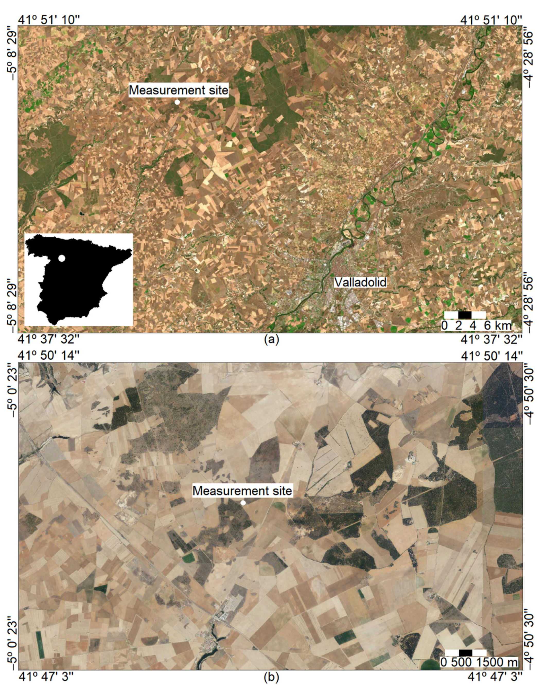
2. Materials and Methods

2.1. CO₂ and CH₄ Observations

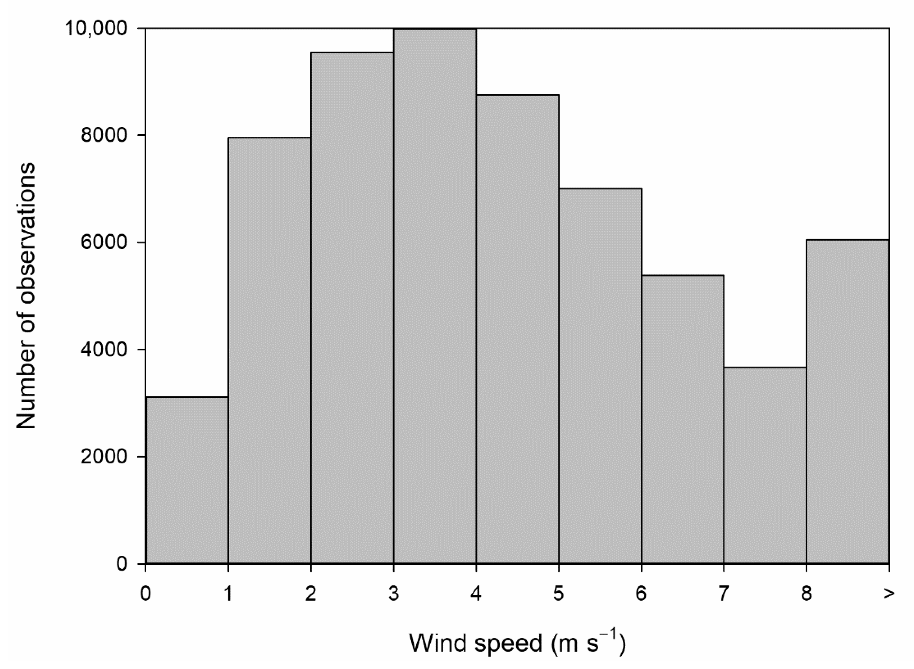
Dry concentrations of both gases were measured with a Picarro G1301 analyser in the centre of the northern plateau of the Iberian Peninsula (CIBA station, 41°48′50″ N, 4°55′59″ W, 852 m a.s.l.). The analysis period covered nine years from October 2010. Although observations were obtained at three levels, only the highest (at 8.25 m a.g.l.) was used in this paper, and hourly averages were calculated.

The measurement site is nearly flat and has no orographic features in its surrounding area. Figure 1 presents the measurement site, which is located in a scrubland area. Landscape is agricultural, and is mainly formed by rainfed crops, and scattered trees are also present. The main nearby city is Valladolid, which lies some 25 km from the measurement site.

2.2. Wind Speed

These data were obtained from the METEX model [20]. A 10 m a.g.l. height was considered since this level is common in meteorological analyses. Although varied wind speed classifications have been suggested following different applications, this paper considers one simple procedure with nine classes. The interval width is 1 m·s⁻¹ until the eighth class, with the last corresponding to wind speeds above 8 m·s⁻¹.

2.3. Theoretical Distributions and Distribution Fitting

Since outliers make the distribution shape different from the Gaussian, seven skewed distributions were used. These are presented in

Table 1. Skewed distributions used in the current study.

Distribution	Probability Density Function	Parameter Calculation
Beta [11]	$f\left(x\right)=\left[\frac{\mathsf{\Gamma }\left(\alpha +\beta \right)}{\mathsf{\Gamma }\left(\alpha \right)\mathsf{\Gamma }\left(\beta \right)}\right]x^{\alpha -1}{\left(1-x\right)}^{\beta -1};0\le x\le 1; \alpha , \beta >0$	$\alpha =\frac{{\overline{x}}^2\left(1-\overline{x}\right)}{s^2}-\overline{x}; \beta =\frac{\alpha \left(1-\overline{x}\right)}{\overline{x}}; \overline{x}=\frac{\overline{y}-a}{b-a};$ $s_x^2=\frac{s_y^2}{{\left(b-a\right)}^2}$
Exponential [21]	$f\left(x\right)=\theta exp\left(-\theta x\right);x>0; \theta >0$	$\theta =1/\overline{x}$
Frechet [22]	$f\left(x\right)=\frac{\lambda }{\sigma }{\left(\frac{\sigma }{x}\right)}^{\lambda +1}exp\left\{-{\left(\frac{\sigma }{x}\right)}^{\lambda }\right\};x\ge 0; \sigma , \lambda >0$	$-ln\left[-ln\left\{F\left(x\right)\right\}\right]=-\lambda \ln \sigma +\lambda \ln \left(x\right)$
Gamma [11]	$f\left(x\right)=\frac{{\left(x/\beta \right)}^{\alpha -1}exp\left(-x/\beta \right)}{\beta \mathsf{\Gamma }\left(\alpha \right)}; x,\alpha , \beta >0$	$D=\ln \left(\overline{x}\right)-\frac{1}{n}{\displaystyle {\displaystyle \sum }_{i=1}^n}\ln \begin{array}{c}\left(x_i\right); \alpha =\frac{1+\sqrt{1+\frac{4D}{3}}}{4D}; \\ \beta =\overline{x}/\alpha \end{array}$
Gumbel [11]	$f\left(x\right)=\frac{1}{\beta }exp\left\{-exp\left[-\frac{\left(x-\zeta \right)}{\beta }\right]-\frac{\left(x-\zeta \right)}{\beta }\right\}$	$\beta =\frac{x\sqrt{6}}{\pi }; \zeta =\overline{x}-\gamma \beta ; \gamma =0.57721$
Lindley [21]	$f\left(x\right)=\frac{{\theta }^2}{\theta +1}\left(1+x\right)e^{-\theta x};x>0, \theta >0$	$\theta =\frac{-\left(\overline{x}-1\right)+\sqrt{{\left(\overline{x}-1\right)}^2+8\overline{x}}}{2\overline{x}}$
Weibull [23]	$f\left(x\right)=\left(\frac{\alpha }{\beta }\right){\left(\frac{x}{\beta }\right)}^{\alpha -1}exp\left[-{\left(\frac{x}{\beta }\right)}^{\alpha }\right];x, \alpha , \beta >0$	$ln\left(-ln\left(1-F\left(x\right)\right)\right)=\alpha ln\left(x\right)-\alpha ln\left(\beta \right)$

. Although nonparametric procedures guarantee satisfactory fits of histograms, certain parametric expressions may be directly fitted and are preferred, since numerical iterations are not required. Moreover, they are flexible enough to successfully describe the observations, have already been theoretically developed, and the application to gas concentrations extends their field of use.

Additionally, distribution agreement with the observations is compared using certain statistics presented in

Table 2. Efficiency criteria.

Name	Equation
Pearson correlation coefficient	$r=\frac{{{\displaystyle \sum }}_{i=1}^n\left(O_i-\overline{O}\right)\left(C_i-\overline{C}\right)}{\sqrt{{{\displaystyle \sum }}_{i=1}^n{\left(O_i-\overline{O}\right)}^2}\sqrt{{{\displaystyle \sum }}_{i=1}^n{\left(C_i-\overline{C}\right)}^2}}$
Willmott index of agreement	$d=1-\frac{{{\displaystyle \sum }}_{i=1}^n{\left(O_i-C_i\right)}^2}{{{\displaystyle \sum }}_{i=1}^N{\left(\left|C_i-\overline{O}\right|+\left|O_i-\overline{O}\right|\right)}^2}$
Modified index of agreement	$d_{mod}=1-\frac{{{\displaystyle \sum }}_{i=1}^n\left|O_i-C_i\right|}{{{\displaystyle \sum }}_{i=1}^N\left(\left|C_i-\overline{O}\right|+\left|O_i-\overline{O}\right|\right)}$
Nash–Sutcliffe efficiency	$E=1-\frac{{{\displaystyle \sum }}_{i=1}^n{\left(O_i-C_i\right)}^2}{{{\displaystyle \sum }}_{i=1}^n{\left(O_i-\overline{O}\right)}^2}$
Modified Nash–Sutcliffe efficiency	$E_{mod}=1-\frac{{{\displaystyle \sum }}_{i=1}^n\left|O_i-C_i\right|}{{{\displaystyle \sum }}_{i=1}^n\left|O_i-\overline{O}\right|}$

, where O corresponds to the observed values, and C to the calculated ones, with the two following objectives. The first is to select the distribution that achieves the best agreement, and the second is to compare the response of the statistics used in order to choose the most sensitive. One of these statistics, the correlation coefficient, is frequently used, although satisfactory values of this coefficient are reached with over- or under-predictions of calculations. However, the rest are statistics that were proposed in order to overcome the restrictions of the correlation coefficient [24].

2.4. Daily and Annual Cycles

These cycles were described by two statistics each hour and each month. The first is the mean, which may be affected by outliers, and the second is the median, which is more robust. Small differences between them reveal a regular distribution of observations whereas a contrast between the mean and the median indicates irregularly placed outliers that may skew the distribution. Moreover, the description of the two cycles was modelled by two procedures. The first is parametric, since it is based on the addition of two harmonic functions, following the equation

$$y=a_0+a_{1}cos\left(\frac{2\pi }{T}t-{\theta }_0\right)+a_{2}cos\left(\frac{4\pi }{T}t-{\theta }_1\right),$$

(1)

where y is the concentration, t is time, and the period of the second harmonic function is the half period of the first harmonic function. The difference between the constants θ₀ and θ₁ allows the symmetry of the first harmonic function to be broken. Both constants, together with the rest of the coefficients a_i, may be calculated by multiple linear regression.

A nonparametric method was also considered, with the following expression being used:

$$y\left(t,h\right)=\frac{{{\displaystyle \sum }}_{i=1}^{n}K\left(\frac{t-t_i}{h}\right)y_i}{{{\displaystyle \sum }}_{i=1}^{n}K\left(\frac{t-t_i}{h}\right)},$$

(2)

where the subscript i denotes the values known, h is the window width, and the Gaussian kernel function was used for the calculations.

$$K\left(x\right)={\left(2\pi \right)}^{-1/2}\exp \left(-0.5x^2\right),$$

(3)

The statistics presented in Table 2 were considered in order to establish the goodness of the fit.

3. Results

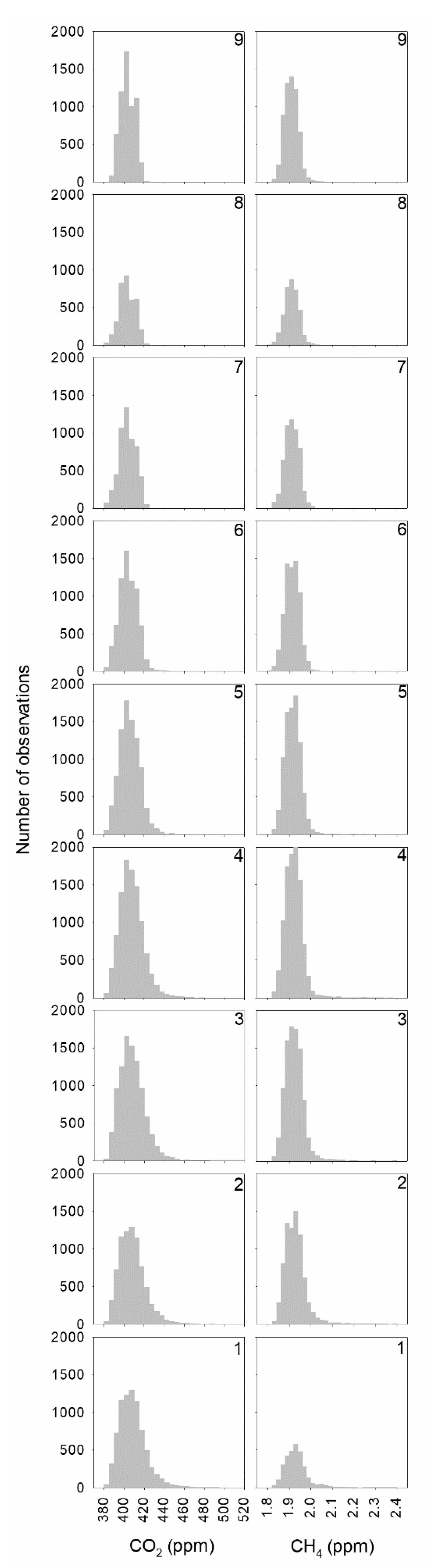
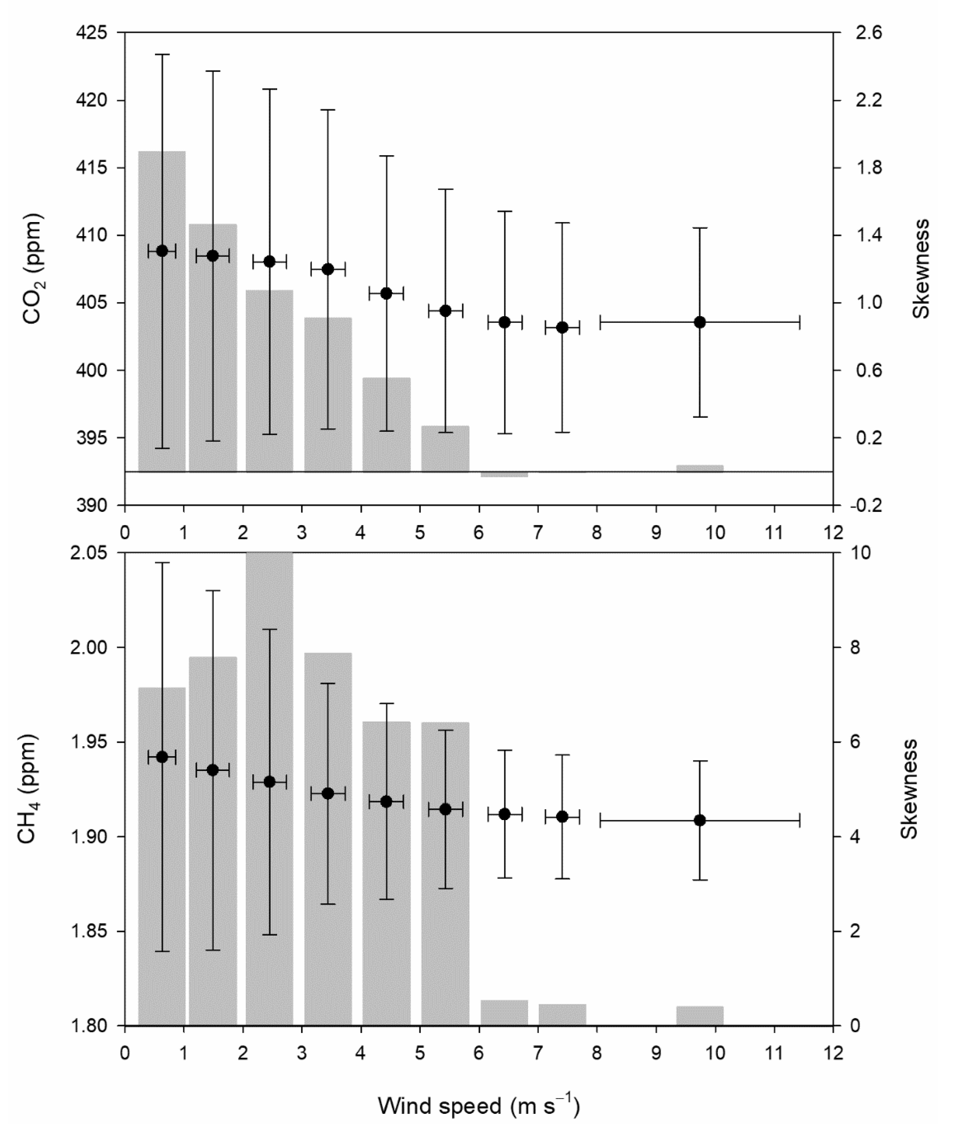
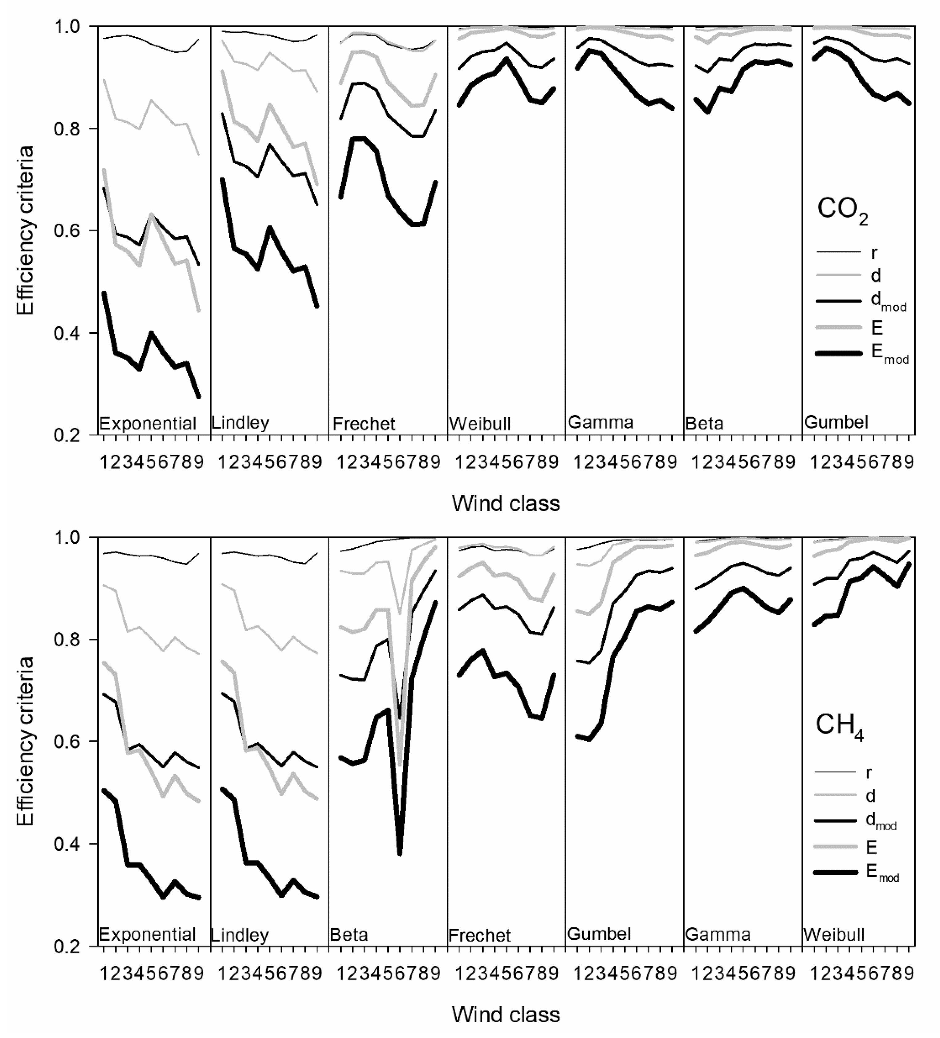
3.1. Wind Speed and Concentration Distributions

The wind speed distribution in 1 m·s⁻¹ intervals is given in Figure 2, which may be satisfactorily described by the Weibull distribution. This figure corresponds to observations where concentration data were available, i.e., around 78% of the period investigated. Observations above 8 m·s⁻¹ are merged in a single class to obtain robust results since outlier analysis lies outside the scope of this paper.

Following this wind classification, concentration histograms are presented in Figure 3. A tail on the right is observed for concentrations at low wind speeds for both gases, such as classes below 5 m·s⁻¹. However, a small tail on the left is also present at high wind speed, between 6 and 8 m·s⁻¹ for CO₂. Figure 4 presents the means and standard deviations of concentrations and wind speed corresponding to wind speed classes as well as the skewness of concentrations. Two intervals with a slight decrease in CO₂ concentration were observed: the first for wind speeds below 4 m·s⁻¹, with a decrease of around 1.3 ppm, and the second until 8 m·s⁻¹, with a decrease of 2.5 ppm. The mean concentration of the last wind speed class is around 0.5 ppm higher than that of the preceding one. Additionally, a gradual decrease in concentration dispersion was observed when wind speed increased. Moreover, skewness also decreased gradually, and even reached negative values in classes 7 and 8. The CH₄ decrease with wind speed was regular. However, its skewness presented a noticeable contrast since it was high until class 6, with one maximum in class 3, although it was very low for the three classes with the highest wind speed. The origin of concentrations of class 1 could be considered local. However, concentrations of class 9 are influenced by transport and could be taken as background concentrations.

Figure 5 presents the efficiency criteria for the distributions used. These were calculated through a comparison between the experimental and the theoretical cumulative distribution functions and were ordered from worst, on the left, to best, on the right. Following these values, the Weibull, Gamma, Beta, and Gumbel distributions offer a similar description for the CO₂ concentrations, with comparable ranges and shapes of efficiency statistics. The range of the statistics decreased gradually from the exponential to the Frechet distribution. For CH₄, the best fits were obtained for the Weibull and Gamma distributions, and the worst for the exponential and Lindley distributions. The decrease in the range of statistics is smoother than that of CO₂. In general, the modified Nash–Sutcliffe efficiency is the statistic with the lowest values, followed by the modified index of agreement. Consequently, both should be used rather than the correlation coefficient, which presents a narrow interval.

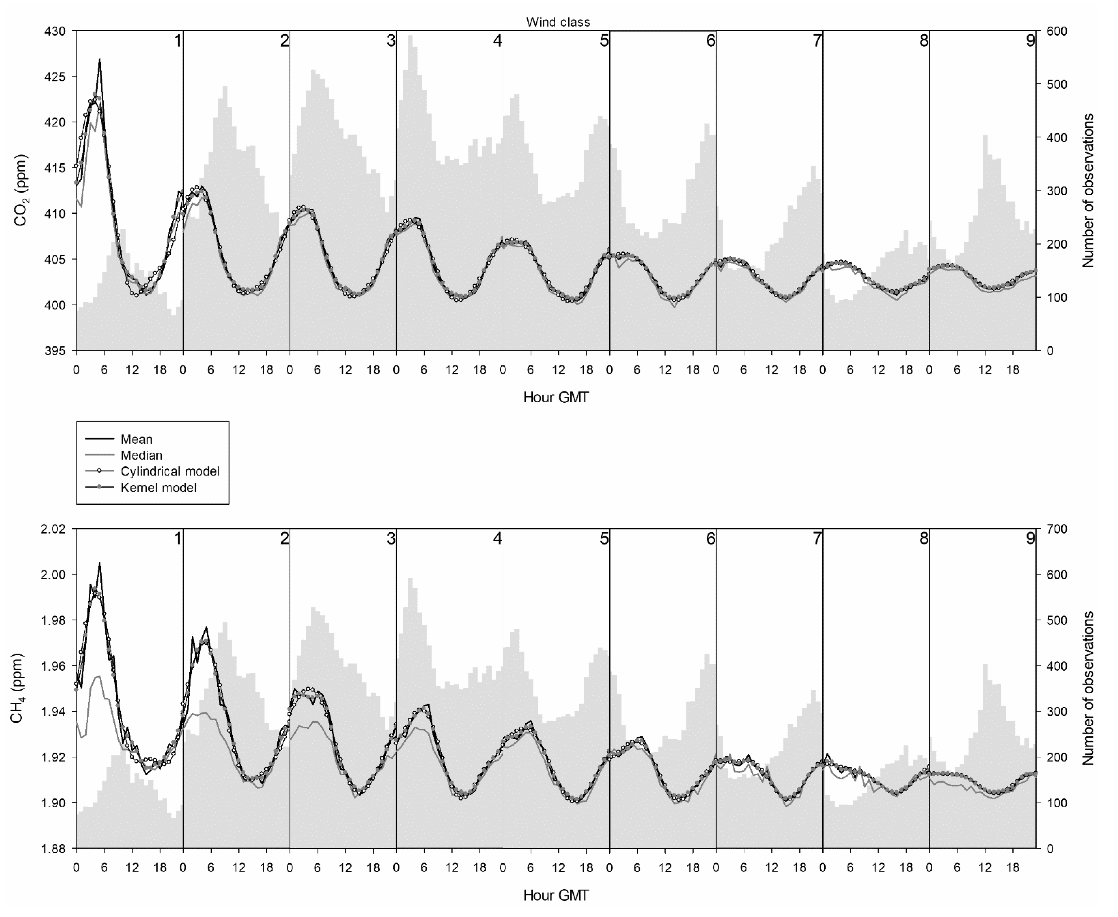
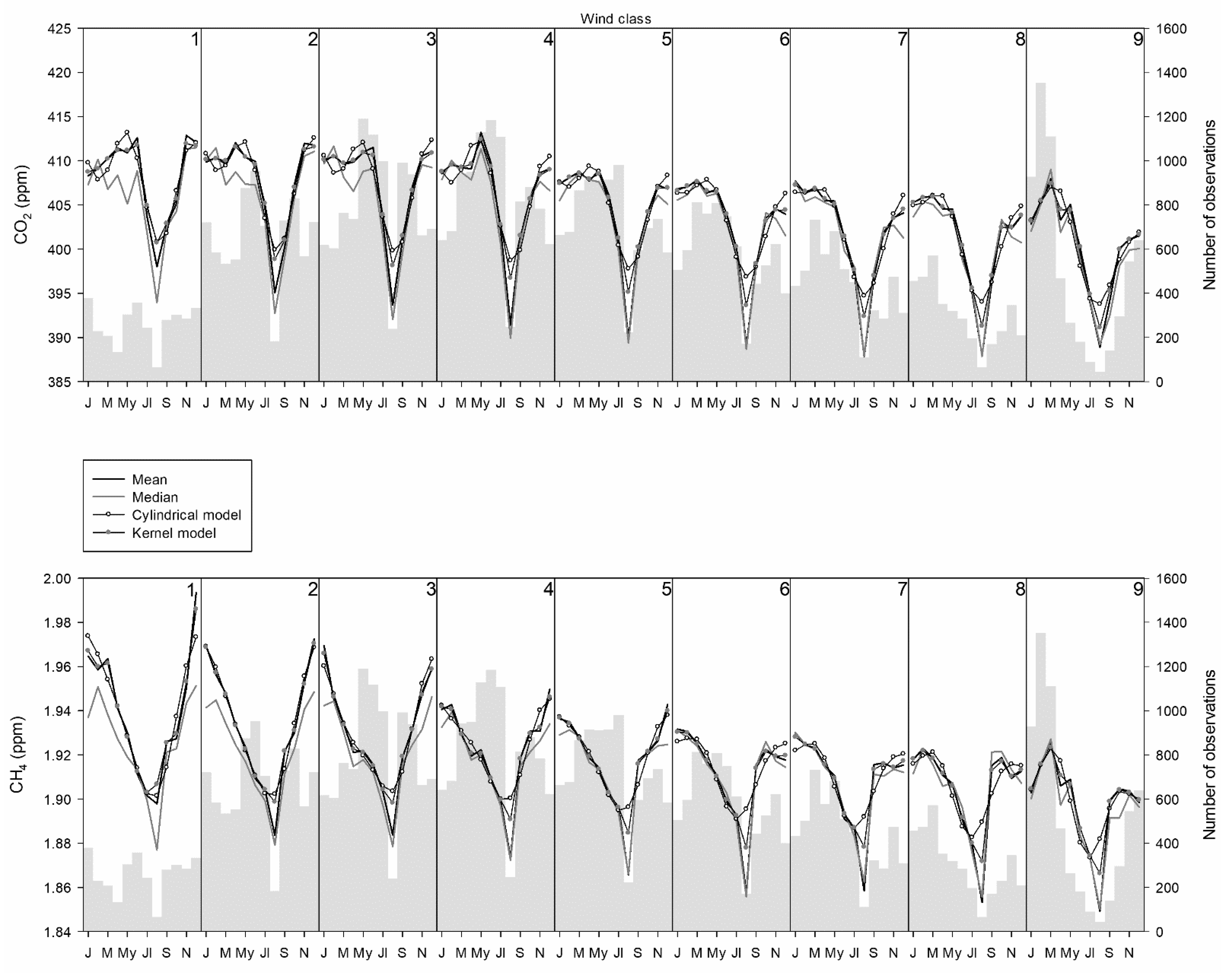
3.2. Daily and Annual Cycles

Figure 6 presents the daily distribution of observations together with the evolution of the median and mean concentrations; this latter one is fitted by the cylindrical and kernel models. A window width, h, is required in this last method, although determining it was not the objective of this paper. Consequently, one hour was fixed following observation availability, and a satisfactory agreement was observed. For low wind speeds below 2 m·s⁻¹ and for the highest wind speeds above 8 m·s⁻¹, the most frequent values are reached at midday. However, at intermediate wind speeds between 2 and 8 m·s⁻¹, the highest frequencies are displaced to late night for low wind speeds, early night for high wind speeds, or during the night for wind speeds from 4 to 6 m·s⁻¹. Mean, median, and modelled values are similar for CO₂, with the highest amplitude of the daily cycle and the highest concentrations occurring after midnight for the lowest wind speed. A similar shape is observed for CH₄, although the contrast between the median and the mean is more noticeable for wind speeds below 3 m·s⁻¹, which may be linked to the frequent outliers of high concentrations at such wind speeds.

Table 3. Statistics used to compare mean and modelled daily cycles.

	CO2		CH4
	Cylindrical	Kernel	Cylindrical	Kernel
r	0.984	0.996	0.974	0.988
d	0.992	0.997	0.987	0.993
dmod	0.923	0.957	0.901	0.930
E	0.969	0.989	0.950	0.974
Emod	0.847	0.916	0.803	0.864

presents the average efficiency statistics when means and modelled values are compared. As in the previous case, when distributions are considered, the modified Nash–Sutcliffe efficiency, followed by the modified index of agreement, achieves the lowest values, and, for both gases, the kernel model fits better than the cylindrical model.

Figure 7 presents the frequency of observations together with the annual cycle of means, medians, and modelled observations. One month was initially suggested for the window width in the annual cycle with the kernel procedure, and a smooth evolution was observed. Consequently, a narrower window equal to half a month was used. Since the equipment was switched off for most of the months of August, the frequencies observed in this month were low. For wind speed below 1 m·s⁻¹, observations are regularly distributed during the year. However, for wind speed from 1 to 3 m·s⁻¹, high frequencies are observed in the central part of the year. For wind speeds from 3 to 7 m·s⁻¹, high frequencies are obtained in the first half of the year, and, finally, for wind speeds above 7 m·s⁻¹, high frequencies are found in the first few months of the year.

Although the lowest concentration of both gases is reached in summer, especially in August, some differences between them are noticeable. Below 5 m·s⁻¹, the interval of low concentrations for CO₂ was narrow, whereas it was prominent in the CH₄ annual cycle, with a gradual decrease in the first half of the year and a gradual increase after summer.

Similar statistics were used to compare the means and modelled values (

Table 4. Statistics used to compare mean and modelled annual cycles.

	CO2		CH4
	Cylindrical	Kernel	Cylindrical	Kernel
r	0.923	0.990	0.890	0.984
d	0.944	0.982	0.919	0.980
dmod	0.814	0.915	0.802	0.919
E	0.828	0.940	0.774	0.937
Emod	0.646	0.840	0.630	0.848

). The pattern of results was similar to that of the daily cycle, with the modified Nash–Sutcliffe efficiency followed by the modified index of agreement being the estimators with the lowest values. As with the distribution fitting, both statistics are sufficiently sensitive to the contrast between the values they evaluate and may be chosen against others that are more frequent, such as the correlation coefficient.

4. Discussion

4.1. Wind Speed

The region of the measurement site is one of the largest in the EU and has one of the lowest population densities, a population which is decreasing even further [25]. The population is mainly rural, and urbanization is low, with Valladolid (around 300,000 inhabitants to the SE of the site, Figure 1) being the largest city in the region. Duarte et al. [26] indicated that CO₂ emissions in Spanish households in 1999 were below the country average for a sparse population density (−12.4%) and for rural sites (−11.2%). Consequently, CO₂ emissions linked with the urban development observed in various Chinese cities [27] may be discarded or considered to have a negligible effect. Even at rural sites in the region, the population is low [28], and its contribution to atmospheric CO₂ may be considered slight when compared to sites where there is a greater contribution of the rural population [29].

Information about the prevailing wind direction at the site for high wind speed was available from Pérez et al. [30], where measurements at 100 m revealed no prevailing wind directions for wind speeds below 4 m·s⁻¹ but two opposite prevailing wind directions for wind speeds between 4 and 15 m·s⁻¹, ENE and WSW, where transport is regional and these directions are not affected by nearby pollution sources. Figure 3 indicates that CO₂ histograms are right-skewed for low wind speed, since noticeable outliers present a local origin. However, distributions are nearly symmetrical or even left-skewed for high wind speeds where prevailing directions are not affected by nearby sources.

The dispersion of values observed in Figure 4 is mainly attributed to the daily evolution presented in Figure 6, since smooth cycles are obtained with high wind speeds, which are linked with low dispersion, whereas cycles with large amplitudes are observed for low wind speeds, which are associated with noticeable dispersion.

The inverse relationship between CO₂ and wind speed has been suggested by different analyses, such as Al-Bayati et al. [31] for satellite observations in Iraq or Dimitriou et al. [32], who also presented CH₄ concentrations in the city of Athens. This latter study considers a scatterplot with seasonal concentrations. The main drawback of such a representation is observation overlapping, which makes it difficult to obtain an average concentration for a wind speed interval. One additional feature is that outliers are prominent, although their contribution to the average concentration may be only slight.

Duan et al. [33] proposed six intervals, five with a width of 1 m·s⁻¹ and the last one for the remaining wind speeds. Boxplots for CO₂ concentrations ranged from 300 to 550 ppm, i.e., they were higher than those used in this study. Medians frequently decreased with wind speed, although in spring the initial decrease was followed by a final increase. Moreover, noticeable interquartile ranges were observed for high wind speeds in summer. Boxplots were also used by Pathakoti et al. [34], who analysed the influence of meteorological parameters on CO₂ at the Indian Antarctic research station. Under these extreme conditions, a width of 5 m·s⁻¹ was used and concentrations remained nearly steady below 20 m·s⁻¹ and only decreased above this wind speed.

Alternative graphs have been used by different authors. Mai et al. [35] analysed CO₂ concentrations at the Pearl River Delta region in China with a plot where seven narrow intervals (width of 0.5 m·s⁻¹) are used and in which the standard deviation of concentrations is included. The decrease in CO₂ concentration reached nearly 20 ppm, with similar concentrations below 2 m·s⁻¹ in autumn. Wei et al. [36] analysed CO₂ and CH₄ concentrations in Shanghai, China, with graphs where box and violin plots were combined. Five wind speed intervals were used with a 1 m·s⁻¹ width and one additional interval for wind speeds above 5 m·s⁻¹. The decrease in concentration for both gases was noticeable for wind speeds below 4 m·s⁻¹, and the increase was slow above this wind speed for CO₂, whereas concentrations remained steady for CH₄. In both cases, the relatively high CO₂ concentrations for high wind speeds were attributed to transport of polluted air masses. The response of CO₂ concentrations to wind speed was similar in Figure 4, revealing the slight contribution of the surroundings at the measurement site.

4.2. Distribution Fitting

The presence of outliers determines skewed distributions. Pérez et al. [37] analysed the skewness of CO₂ concentration using a range of statistics. Among them, the Yule coefficient was selected following the relationship between skewness and the daily evolution of concentrations. Although global distribution was right-skewed, left-skewed distributions prevailed at midday. Moreover, the influence of wind speed on skewness revealed low, and even negative, values for high wind speeds.

Skewed functions expand the field of application of symmetric functions both in spatial and temporal research. They were used by Pérez et al. [38] in a spatial analysis of CO₂ concentrations to investigate the impact of the Valladolid urban plume at this rural site by its extension, around 135 degrees, and magnitude, slightly below 10 ppm. Differences among the functions considered included the place of the tail and the flatness of the curve. Various statistics were used in the study to select the cubic function, followed by the gamma and Weibull distributions as the most suitable to fit urban plume concentrations. Moreover, skewed functions were also used by Pérez et al. [39] to investigate the daily cycle of CO₂ concentrations. In this case, the best fit was obtained with the generalised von Mises function.

Pérez et al. [17] fitted CO₂ concentration histograms to 14 skewed distributions. Parameter calculation was performed with equations established using analytical procedures in nine of them. However, the rest were obtained by numerical procedures. These are iterative methods that slow down the calculation. The current analysis retains typical distributions and considers certain functions, such as the Frechet and Lindley functions, which have not been used to date. Moreover, parameter calculation is direct, since numerical procedures are avoided.

Perez et al. [38] used 12 statistics to compare calculated and observed concentrations. Moreover, since the ranges of these statistics differ substantially and the response of each equation may be different to each statistic, they were combined into one comprehensive metric proposed by Zhou et al. [40] where each statistic has the same weight. In the current analysis, two of these statistics, the correlation coefficient and the index of agreement, were retained. However, the Nash–Sutcliffe efficiency and the modified forms of the index of agreement and the Nash–Sutcliffe efficiency are statistics that have scarcely been explored in the context of this study.

4.3. Fitting of Daily and Annual Cycles

Harmonic functions are usually used to describe the annual evolution of the gases considered in this study. This is a parametric procedure with substantial flexibility since the number of harmonics is variable and usually ranges from the simplest method, with only one harmonic [41], to the most complex one, with four harmonics [42,43].

CO₂ and CH₄ annual cycles at remote and rural sites frequently present a minimum in summer attributed to low plant and soil activity [44]. However, the shape of this cycle depends on the site, since even remote places may be affected by pollution transport. This is the case of certain high concentration events recorded at some European high-altitude stations, such as Zugspitze in Germany, attributed to the atmospheric circulation that carries polluted air from the European plains to the Alpine stations [45,46]. Moreover, high CH₄ values observed in summer at Mount Waliguan, China, revealed the agricultural source, rice growing, of CH₄ [47].

Parameterisation of these cycles should be adapted to each measurement station. However, even for the simplest cycles, the one harmonic evolution may be considered as an initial approximation, since a six-month period between the maximum and the minimum is difficult to achieve [48,49]. Pérez et al. [19] tried different combinations of four harmonics and recommended using the first and second harmonics as a simple enough and complete enough equation to accurately describe CO₂ and CH₄ annual evolution. Moreover, the CO₂ cycle was already fitted by a two-harmonic function and kernel calculations by Pérez et al. [50].

Fernández-Duque et al. [51] considered six kernel functions to fit both the trend and the annual evolution of CO₂ and CH₄. Although the Gaussian kernel provided low fits for the trend, agreement increased for the annual cycle. In this study, the relationship between observed and calculated values was satisfactory for both daily and annual cycles, as presented in Figure 6 and Figure 7 and in Table 3 and Table 4.

Pérez et al. [52] analysed the influence of four meteorological variables, boundary layer height, recirculation factor, wind direction, and wind speed, on the CO₂ and CH₄ annual cycle. Varied wind speed thresholds were used, and concentrations were analysed at night. Differences between average concentrations for observations above the highest threshold, 9 m·s⁻¹, and all observations at night were around −1% for CO₂ and CH₄. However, when observations below the lowest threshold, 2 m·s⁻¹, are selected, these differences are around 0.9 and 0.7%, for CO₂ and CH₄, respectively. The current analysis does not consider thresholds but rather wind speed intervals. The contrast between the average values calculated for the extreme intervals is around 2% for both gases.

5. Conclusions

The current study focuses on the relationship between CO₂ and CH₄ concentrations measured at a rural site and wind speed during nine years of observations.

Nine wind speed intervals were suggested, and the response of the mean CO₂ concentrations revealed three groups: the first, below 4 m·s⁻¹ with a slow decrease; the second, of wind speeds up to below 8 m·s⁻¹, with a greater influence of wind speed; and the third, for wind speeds above 9 m·s⁻¹, with concentrations that are only slightly greater than those of the interval 7–8 m·s⁻¹, which could be attributed to background concentrations transported by wind. The concentration decrease with the increase in wind speed was more gradual for CH₄ than for CO₂.

Although concentration skewness was mainly positive due to outliers linked to stable stratification, close to zero or even negative skewness was observed in wind speed intervals above 6 m·s⁻¹. These distributions may be only slightly affected by outliers owing to prevailing transport by wind, with the skewness contrast being noticeable for CH₄.

Seven skewed distributions were used to fit the concentrations. Moreover, five efficiency criteria were considered. The most sensitive statistic was the modified Nash–Sutcliffe efficiency, with the correlation coefficient being the least sensitive. The Gumbel was the most suitable distribution function for CO₂, followed by very similar fits for the gamma and beta distributions. The Weibull distribution presented the best fit for CH₄. In contrast, the worst fit was for the exponential distribution.

Analysis of the daily cycle revealed the most frequent observations at midday for low wind speeds. Moreover, the daily cycle amplitude gradually decreased following the increase in wind speed, with the daily cycle being fairly slight for winds above 9 m·s⁻¹.

Noticeable minima were observed in summer for both gases, with the drop in concentration being more marked for CO₂. The contrast between the mean and median concentrations was noticeable for low wind speeds and could be attributed to the distribution shape and outlier influence. Although the mean concentration decreased with the increase in wind speed, the change in the annual cycle amplitude was less pronounced than that of the daily cycle. Moreover, CO₂ amplitude was greater above 9 m·s⁻¹ than below 2 m·s⁻¹.

This research improves current knowledge of the relationship between wind speed and CO₂ and CH₄, although a more detailed analysis, such as the seasonal response of this relationship or directional studies, may be the subject of future research. In addition, combining observed and modelled measurements has proved successful and may be used when there is a sufficient number of observations, although its application with isolated measurements should be explored. Finally, these are promising research lines vis à vis obtaining better insights into the influence of meteorological variables on the concentrations of the two greenhouse gases studied.

References

1. European Environment Agency. Household Energy Consumption. Available online: https://www.eea.europa.eu/airs/2018/resource-efficiency-and-low-carbon-economy/household-energy-consumption (accessed on 28 July 2021).
2. Dong, Z.; Wang, S.; Xing, J.; Chang, X.; Ding, D.; Zheng, H. Regional transport in Beijing-Tianjin-Hebei region and its changes during 2014–2017: The impacts of meteorology and emission reduction. Sci. Total Environ. 2020, 737, 139792. [Google Scholar] [CrossRef]
3. Mousavinezhad, S.; Choi, Y.; Pouyaei, A.; Ghahremanloo, M.; Nelson, D.L. A comprehensive investigation of surface ozone pollution in China, 2015–2019: Separating the contributions from meteorology and precursor emissions. Atmos. Res. 2021, 257, 105599. [Google Scholar] [CrossRef]
4. Li, Y.; Miao, Y.; Che, H.; Liu, S. On the heavy aerosol pollution and its meteorological dependence in Shandong province, China. Atmos. Res. 2021, 256, 105572. [Google Scholar] [CrossRef]
5. Liu, Y.; Zhou, Y.; Lu, J. Exploring the relationship between air pollution and meteorological conditions in China under environmental governance. Sci. Rep. 2020, 10, 14518. [Google Scholar] [CrossRef]
6. Miao, Y.; Che, H.; Zhang, X.; Liu, S. Relationship between summertime concurring PM2.5 and O3 pollution and boundary layer height differs between Beijing and Shanghai, China. Environ. Pollut. 2021, 268, 115775. [Google Scholar] [CrossRef]
7. Yoshino, A.; Takami, A.; Hara, K.; Nishita-Hara, C.; Hayashi, M.; Kaneyasu, N. Contribution of local and transboundary air pollution to the urban air quality of Fukuoka, Japan. Atmosphere 2021, 12, 431. [Google Scholar] [CrossRef]
8. Liu, Z.; Shen, L.; Yan, C.; Du, J.; Li, Y.; Zhao, H. Analysis of the influence of precipitation and wind on PM2.5 and PM10 in the atmosphere. Adv. Meteorol. 2020, 2020, 5039613. [Google Scholar] [CrossRef]
9. Massen, F.; Beck, E.G. Accurate estimation of CO2 background level from near ground measurements at non-mixed environments. In The Economic, Social and Political Elements of Climate Change. Climate Change Management; Leal Filho, W., Ed.; Springer: Berlin/Heidelberg, Germany, 2011; pp. 509–522. [Google Scholar] [CrossRef]
10. García, M.A.; Sánchez, M.L.; Pérez, I.A. Differences between carbon dioxide levels over suburban and rural sites in Northern Spain. Environ. Sci. Pollut. Res. 2012, 19, 432–439. [Google Scholar] [CrossRef]
11. Wilks, S. Statistical Methods in the Atmospheric Sciences, 4th ed.; Elsevier: Amsterdam, The Netherlands, 2019; p. 840. [Google Scholar]
12. Solovyova, T.V.; Nasimi, M.H.; Tertischnikov, I.V. On the pollution of the atmosphere of the city of Kabul with fine dust. IOP Conf. Ser. Earth Environ. Sci. 2019, 272, 022148. [Google Scholar] [CrossRef]
13. Zhang, K.; Zhao, C.; Fan, H.; Yang, Y.; Sun, Y. Toward understanding the differences of PM2.5 characteristics among five China urban cities. Asia-Pac. J. Atmos. Sci. 2020, 56, 493–502. [Google Scholar] [CrossRef]
14. El Genidy, M.M.; Ali, A.K. Modeling the amount of pollutants ozone using moments method and generalized extreme value distribution. Asian J. Sci. Res. 2016, 9, 143–151. [Google Scholar] [CrossRef] [Green Version]
15. Mokhtar, M.I.Z.; Ghazali, N.A.; Nasir, M.Y.; Suhaimi, N. Modelling distribution function of surface ozone concentration for selected suburban areas in Malaysia. Malays. J. Anal. Sci. 2016, 20, 863–869. [Google Scholar] [CrossRef]
16. Nasir, M.Y.; Ghazali, N.A.; Mokhtar, M.I.Z.; Suhaimi, N. Fitting statistical distributions functions on ozone concentration data at coastal areas. Malays. J. Anal. Sci. 2016, 20, 551–559. [Google Scholar] [CrossRef]
17. Pérez, I.A.; Sánchez, M.L.; García, M.A.; Pardo, N. Carbon dioxide at an unpolluted site analysed with the smoothing kernel method and skewed distributions. Sci. Total Environ. 2013, 456, 239–245. [Google Scholar] [CrossRef]
18. Pérez, I.A.; Sánchez, M.L.; García, M.A.; Pardo, N. Daily patterns of CO2 in the lower atmosphere of a rural site. Theor. Appl. Climatol. 2015, 122, 195–205. [Google Scholar] [CrossRef]
19. Pérez, I.A.; Sánchez, M.L.; García, M.A.; Pardo, N.; Fernández-Duque, B. Statistical analysis of the CO2 and CH4 annual cycle on the northern plateau of the Iberian Peninsula. Atmosphere 2020, 11, 769. [Google Scholar] [CrossRef]
20. Zeng, J.; Matsunaga, T.; Mukai, H. METEX-A flexible tool for air trajectory calculation. Environ. Modell. Softw. 2010, 25, 607–608. [Google Scholar] [CrossRef]
21. Ghitany, M.E.; Atieh, B.; Nadarajah, S. Lindley distribution and its application. Math. Comput. Simul. 2008, 78, 493–506. [Google Scholar] [CrossRef]
22. Bury, K. Statistical Distributions in Engineering; Cambridge University Press: Cambridge, UK, 1999; pp. 294–310. [Google Scholar]
23. Akdaǧ, S.A.; Dinler, A. A new method to estimate Weibull parameters for wind energy applications. Energy Conv. Manag. 2009, 50, 1761–1766. [Google Scholar] [CrossRef]
24. Krause, P.; Boyle, D.P.; Bäse, F. Comparison of different efficiency criteria for hydrological model assessment. Adv. Geosci. 2005, 5, 89–97. [Google Scholar] [CrossRef] [Green Version]
25. Eurostat. Regions in Europe. Available online: https://ec.europa.eu/eurostat/cache/digpub/regions/ (accessed on 28 July 2021).
26. Duarte, R.; Mainar, A.; Sánchez-Chóliz, J. Social groups and CO2 emissions in Spanish households. Energy Policy 2012, 44, 441–450. [Google Scholar] [CrossRef]
27. Zhang, W.; Jiang, L.; Cui, Y.; Xu, Y.; Wang, C.; Yu, J.; Streets, D.G.; Lin, B. Effects of urbanization on airport CO2 emissions: A geographically weighted approach using nighttime light data in China. Resour. Conserv. Recycl. 2019, 150, 104454. [Google Scholar] [CrossRef]
28. Eurostat. Population Grids. Available online: https://ec.europa.eu/eurostat/statistics-explained/index.php?title=Population_grids#Grid_statistics (accessed on 28 July 2021).
29. Zhang, W.; Wang, C.; Zhang, L.; Xu, Y.; Cui, Y.; Lu, Z.; Streets, D.G. Evaluation of the performance of distributed and centralized biomass technologies in rural China. Renew. Energy 2018, 125, 445–455. [Google Scholar] [CrossRef]
30. Pérez, I.A.; García, M.A.; Sánchez, M.L.; de Torre, B. Analysis of height variations of sodar-derived wind speeds in Northern Spain. J. Wind Eng. Ind. Aerodyn. 2004, 92, 875–894. [Google Scholar] [CrossRef]
31. Al-Bayati, R.M.; Adeeb, H.Q.; Al-Salihi, A.M.; Al-Timimi, Y.K. The relationship between the concentration of carbon dioxide and wind using GIS. AIP Conf. Proc. 2020, 2290, 0027402. [Google Scholar] [CrossRef]
32. Dimitriou, K.; Bougiatioti, A.; Ramonet, M.; Pierros, F.; Michalopoulos, P.; Liakakou, E.; Solomos, S.; Quehe, P.Y.; Delmotte, M.; Gerasopoulos, E.; et al. Greenhouse gases (CO2 and CH4) at an urban background site in Athens, Greece: Levels, sources and impact of atmospheric circulation. Atmos. Environ. 2021, 253, 118372. [Google Scholar] [CrossRef]
33. Duan, Z.; Yang, Y.; Wang, L.; Liu, C.; Fan, S.; Chen, C.; Tong, Y.; Lin, X.; Gao, Z. Temporal characteristics of carbon dioxide and ozone over a rural-cropland area in the Yangtze River Delta of eastern China. Sci. Total Environ. 2021, 757, 143750. [Google Scholar] [CrossRef]
34. Pathakoti, M.; Gaddamidi, S.; Gharai, B.; Sudhakaran Syamala, P.; Rao, P.V.N.; Choudhury, S.B.; Raghavendra, K.V.; Dadhwal, V.K. Influence of meteorological parameters on atmospheric CO2 at Bharati, the Indian Antarctic research station. Polar Res. 2018, 37, 1442072. [Google Scholar] [CrossRef] [Green Version]
35. Mai, B.; Deng, X.; Liu, X.; Li, T.; Guo, J.; Ma, Q. The climatology of ambient CO2 concentrations from long-term observation in the Pearl River Delta region of China: Roles of anthropogenic and biogenic processes. Atmos. Environ. 2021, 251, 118266. [Google Scholar] [CrossRef]
36. Wei, C.; Wang, M.; Fu, Q.; Dai, C.; Huang, R.; Bao, Q. Temporal characteristics of greenhouse gases (CO2 and CH4) in the megacity Shanghai, China: Association with air pollutants and meteorological conditions. Atmos. Res. 2020, 235, 104759. [Google Scholar] [CrossRef]
37. Pérez, I.A.; Sánchez, M.L.; García, M.A.; Ozores, M.; Pardo, N. Analysis of carbon dioxide concentration skewness at a rural site. Sci. Total Environ. 2014, 476, 158–164. [Google Scholar] [CrossRef]
38. Pérez, I.A.; Sánchez, M.L.; García, M.A.; Pardo, N. Analysis and fit of surface CO2 concentrations at a rural site. Environ. Sci. Pollut. Res. 2012, 19, 3015–3027. [Google Scholar] [CrossRef] [PubMed]
39. Pérez, I.A.; Sánchez, M.L.; García, M.A.; Pardo, N. Analysis of CO2 daily cycle in the low atmosphere at a rural site. Sci. Total Environ. 2012, 431, 286–292. [Google Scholar] [CrossRef]
40. Zhou, J.; Erdem, E.; Li, G.; Shi, J. Comprehensive evaluation of wind speed distribution models: A case study for North Dakota sites. Energy Conv. Manag. 2010, 51, 1449–1458. [Google Scholar] [CrossRef]
41. Liu, M.; Wu, J.; Zhu, X.; He, H.; Jia, W.; Xiang, W. Evolution and variation of atmospheric carbon dioxide concentration over terrestrial ecosystems as derived from eddy covariance measurements. Atmos. Environ. 2015, 114, 75–82. [Google Scholar] [CrossRef] [Green Version]
42. Fang, S.X.; Tans, P.P.; Dong, F.; Zhou, H.; Luan, T. Characteristics of atmospheric CO2 and CH4 at the Shangdianzi regional background station in China. Atmos. Environ. 2016, 131, 1–8. [Google Scholar] [CrossRef]
43. Vermeulen, A.T.; Hensen, A.; Popa, M.E.; Van Den Bulk, W.C.M.; Jongejan, P.A.C. Greenhouse gas observations from Cabauw Tall Tower (1992–2010). Atmos. Meas. Tech. 2011, 4, 617–644. [Google Scholar] [CrossRef] [Green Version]
44. Curcoll, R.; Camarero, L.; Bacardit, M.; Àgueda, A.; Grossi, C.; Gacia, E.; Font, A.; Morguí, J.A. Atmospheric Carbon Dioxide variability at Aigüestortes, Central Pyrenees, Spain. Reg. Environ. Chang. 2019, 19, 313–324. [Google Scholar] [CrossRef] [Green Version]
45. Ferrarese, S.; Apadula, F.; Bertiglia, F.; Cassardo, C.; Ferrero, A.; Fialdini, L.; Francone, C.; Heltai, D.; Lanza, A.; Longhetto, A.; et al. Inspection of high–concentration CO2 events at the Plateau Rosa Alpine station. Atmos. Pollut. Res. 2015, 6, 415–427. [Google Scholar] [CrossRef] [Green Version]
46. Ghasemifard, H.; Vogel, F.R.; Yuan, Y.; Luepke, M.; Chen, J.; Ries, L.; Leuchner, M.; Schunk, C.; Vardag, S.N.; Menzel, A. Pollution events at the high-altitude mountain site Zugspitze-Schneefernerhaus (2670 m a.s.l.), Germany. Atmosphere 2019, 10, 330. [Google Scholar] [CrossRef] [Green Version]
47. Zhang, F.; Zhou, L.X.; Xu, L. Temporal variation of atmospheric CH4 and the potential source regions at Waliguan, China. Sci. China-Earth Sci. 2013, 56, 727–736. [Google Scholar] [CrossRef]
48. Pu, J.J.; Xu, H.H.; He, J.; Fang, S.X.; Zhou, L.X. Estimation of regional background concentration of CO2 at Lin’an Station in Yangtze River Delta, China. Atmos. Environ. 2014, 94, 402–408. [Google Scholar] [CrossRef]
49. Uglietti, C.; Leuenberger, M.; Brunner, D. European source and sink areas of CO2 retrieved from Lagrangian transport model interpretation of combined O2 and CO2 measurements at the high alpine research station Jungfraujoch. Atmos. Chem. Phys. 2011, 11, 8017–8036. [Google Scholar] [CrossRef] [Green Version]
50. Pérez, I.A.; Sánchez, M.L.; García, M.A.; Pardo, N. Features of the annual evolution of CO2 and CH4 in the atmosphere of a Mediterranean climate site studied using a nonparametric and a harmonic function. Atmos. Pollut. Res. 2016, 7, 1013–1021. [Google Scholar] [CrossRef] [Green Version]
51. Fernández-Duque, B.; Pérez, I.A.; García, M.A.; Pardo, N.; Sánchez, M.L. Annual and seasonal cycles of CO2 and CH4 in a Mediterranean Spanish environment using different kernel functions. Stoch. Environ. Res. Risk Assess. 2019, 33, 915–930. [Google Scholar] [CrossRef]
52. Pérez, I.A.; Sánchez, M.L.; García, M.A.; Pardo, N. Sensitivity of CO2 and CH4 annual cycles to different meteorological variables at a rural site in northern Spain. Adv. Meteorol. 2019, 2019, 9240568. [Google Scholar] [CrossRef] [Green Version]
Figure 1. (a) Location of the measurement site and the main urban site, Valladolid. Bottom left is the location of the measurement site in Spain. (b) Surrounding area of the measurement site, formed mainly by crops. Images courtesy of © ign.es.
Ijerph 18 08397 g001
Figure 2. Wind speed distribution.
Ijerph 18 08397 g002
Figure 3. Concentration histograms following the wind speed classification.
Ijerph 18 08397 g003
Figure 4. Means, standard deviations, and skewnesses of the concentrations.
Ijerph 18 08397 g004
Figure 5. Distribution functions ordered following the efficiency criteria.
Ijerph 18 08397 g005
Figure 6. Daily cycle following the wind speed classification.
Ijerph 18 08397 g006
Figure 7. Annual cycle following the wind speed classification.
Ijerph 18 08397 g007