
Qualitative Study on the Observations of Emissions, Transport, and the Influence of Climatic Factors from Sugarcane Burning: A South African Perspective

 , , and
Abstract
:
1. Introduction
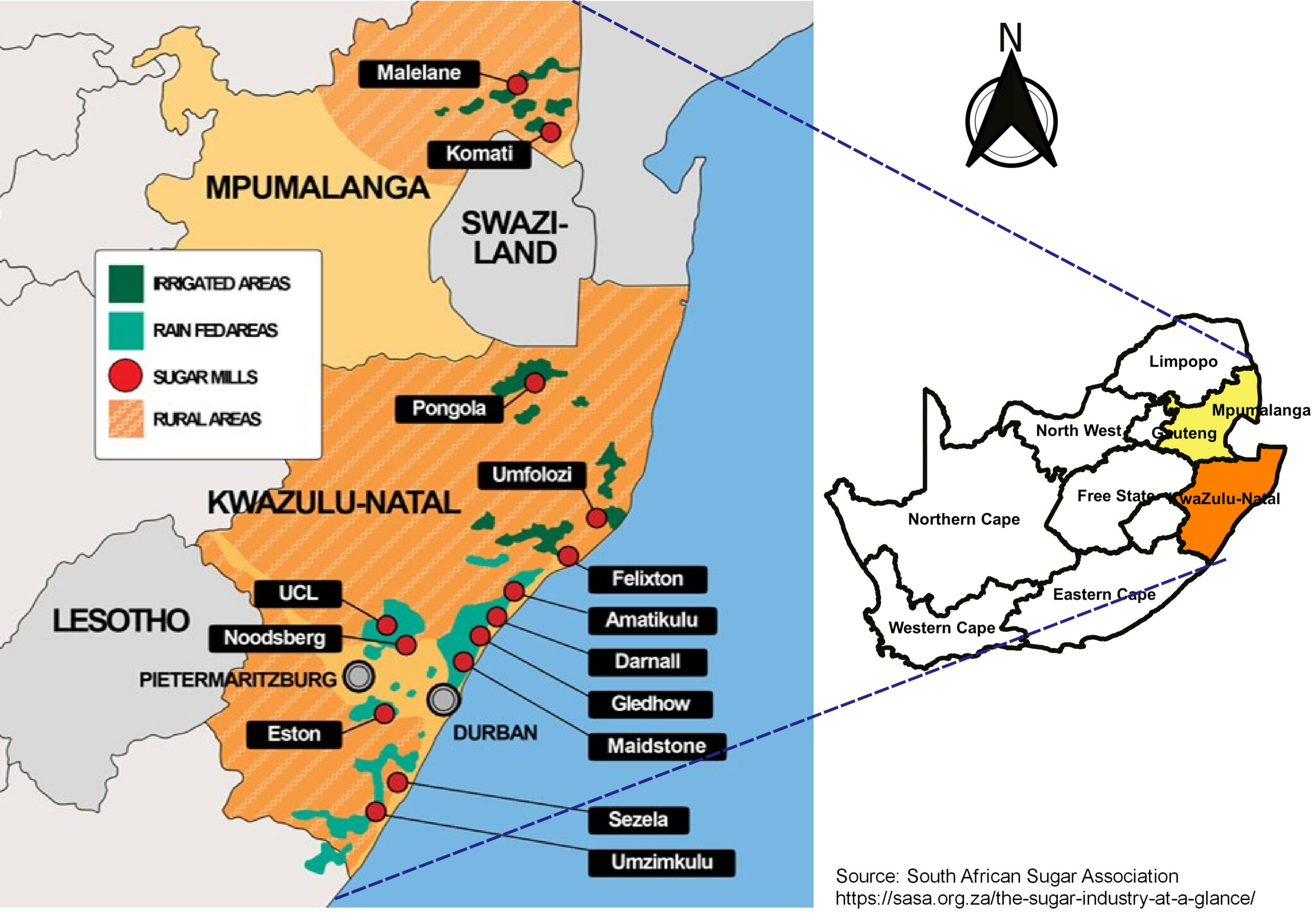
2. Study Area
3. Data and Methods
3.1. MERRA-2
3.2. CALIPSO
3.3. AIRS
3.4. TRMM
3.5. HYSPLIT Model
3.6. SQ–MK Test
- At each comparison, the number of cases xi > xj is counted and indicated by , where xi (i = 1, 2, … n) and xj (1, 2, … n) are the sequential values in a series, respectively.
- The test statistic ti is calculated by
- The mean E(t) and the variance var(ti) of the test statistic are calculated by
- Sequential progressive value can be calculated as
3.7. Surface Rainfall Data
4. Results and Discussions
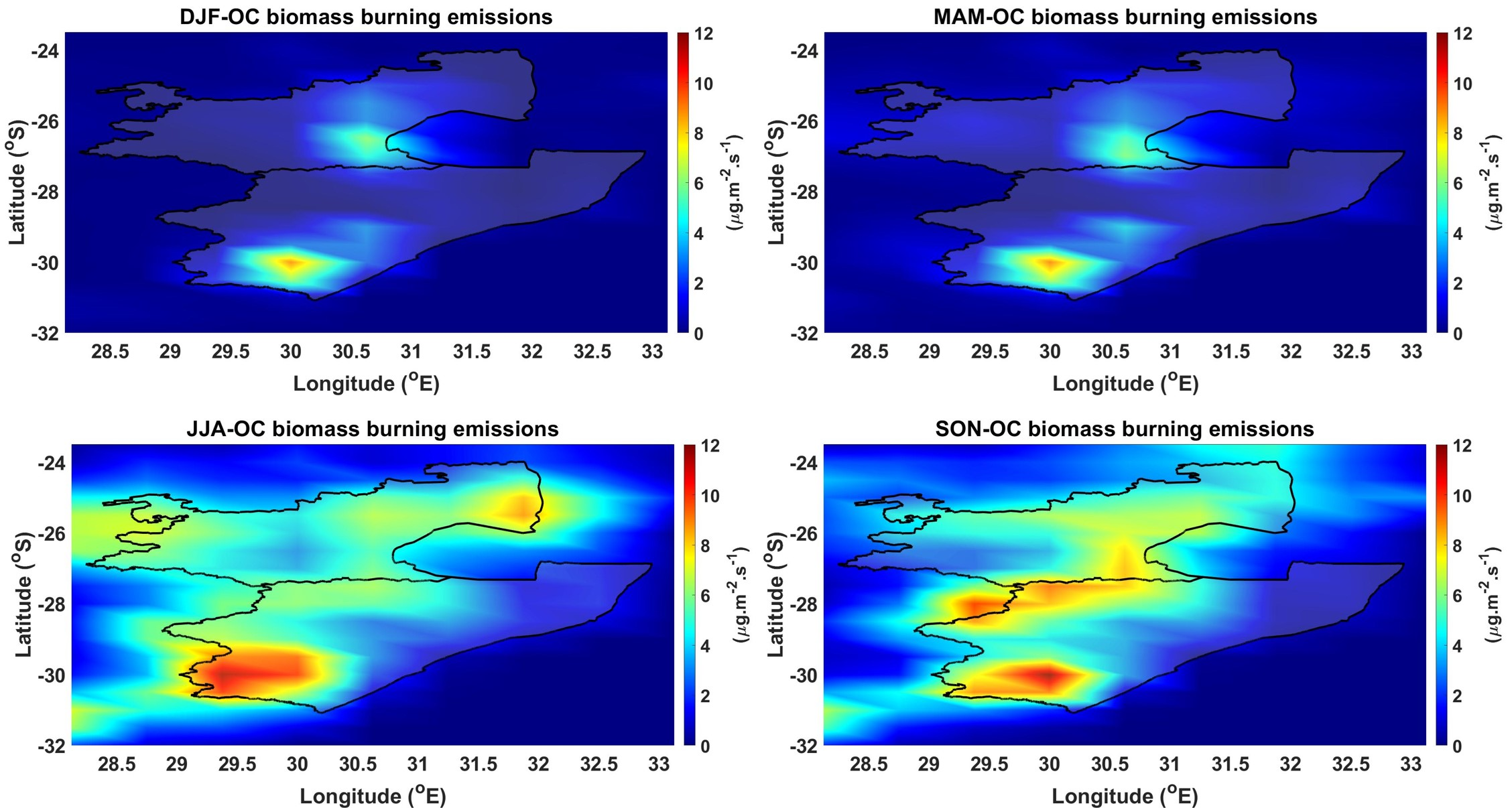
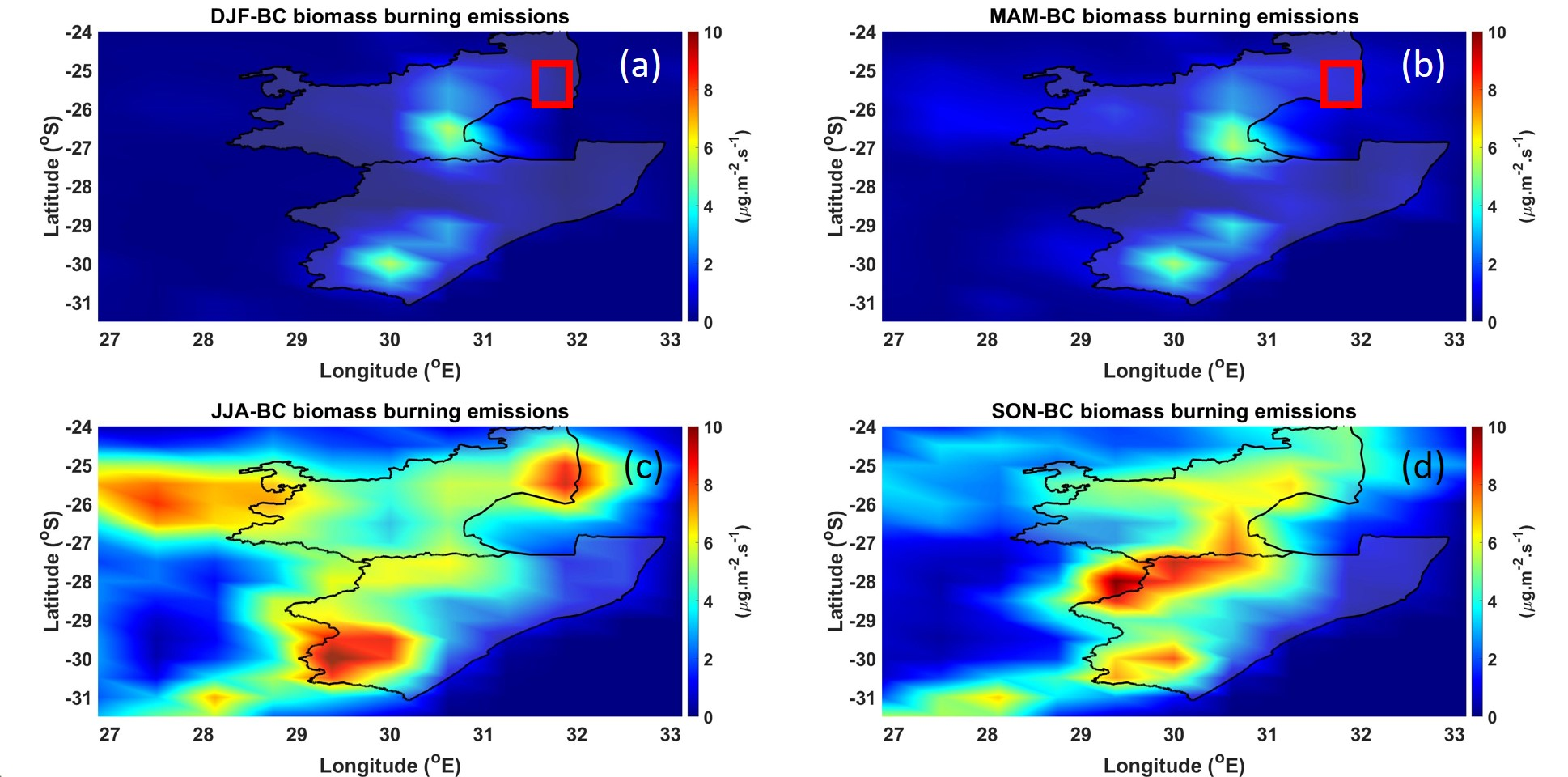
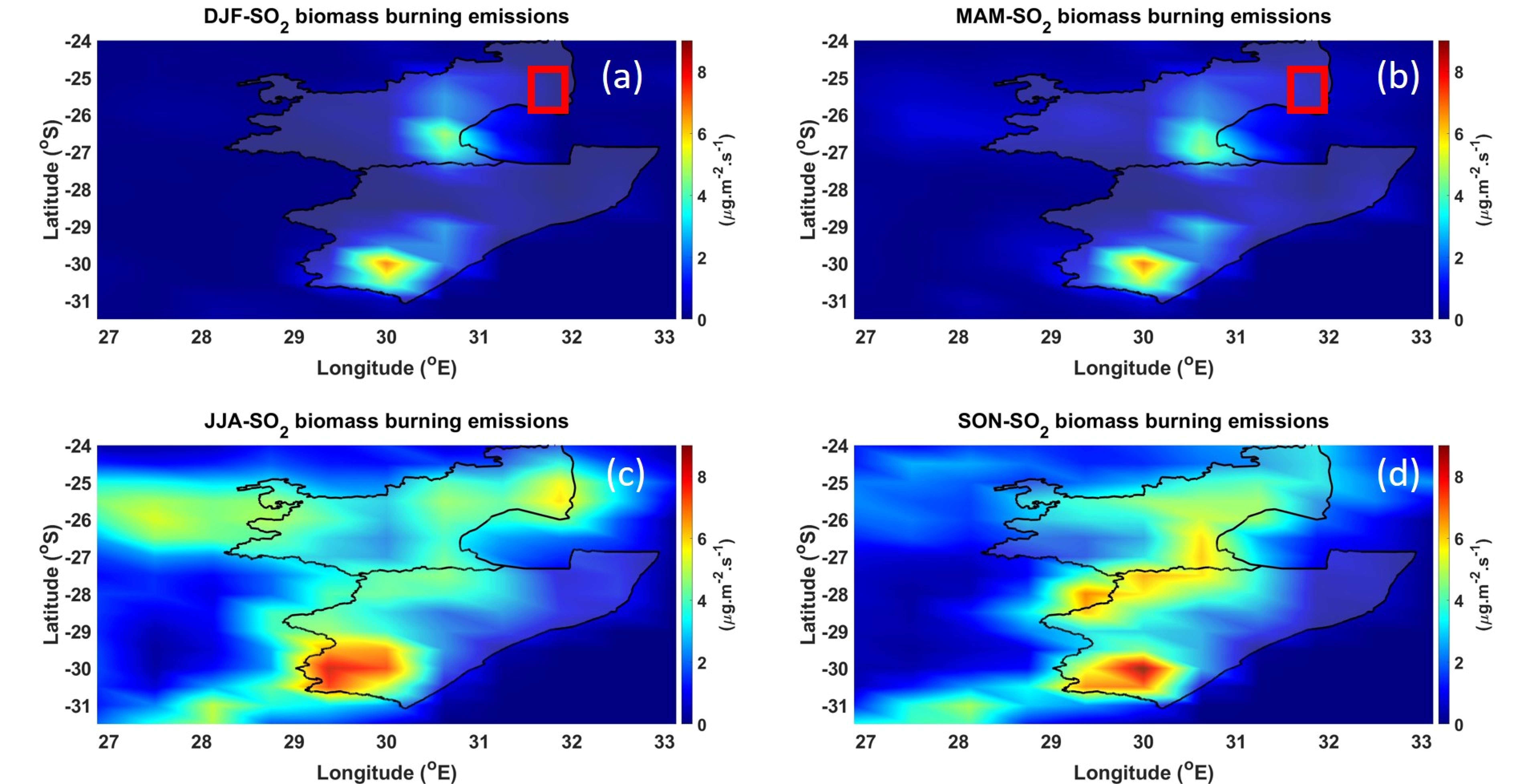
4.1. Emissions from Sugarcane Burning
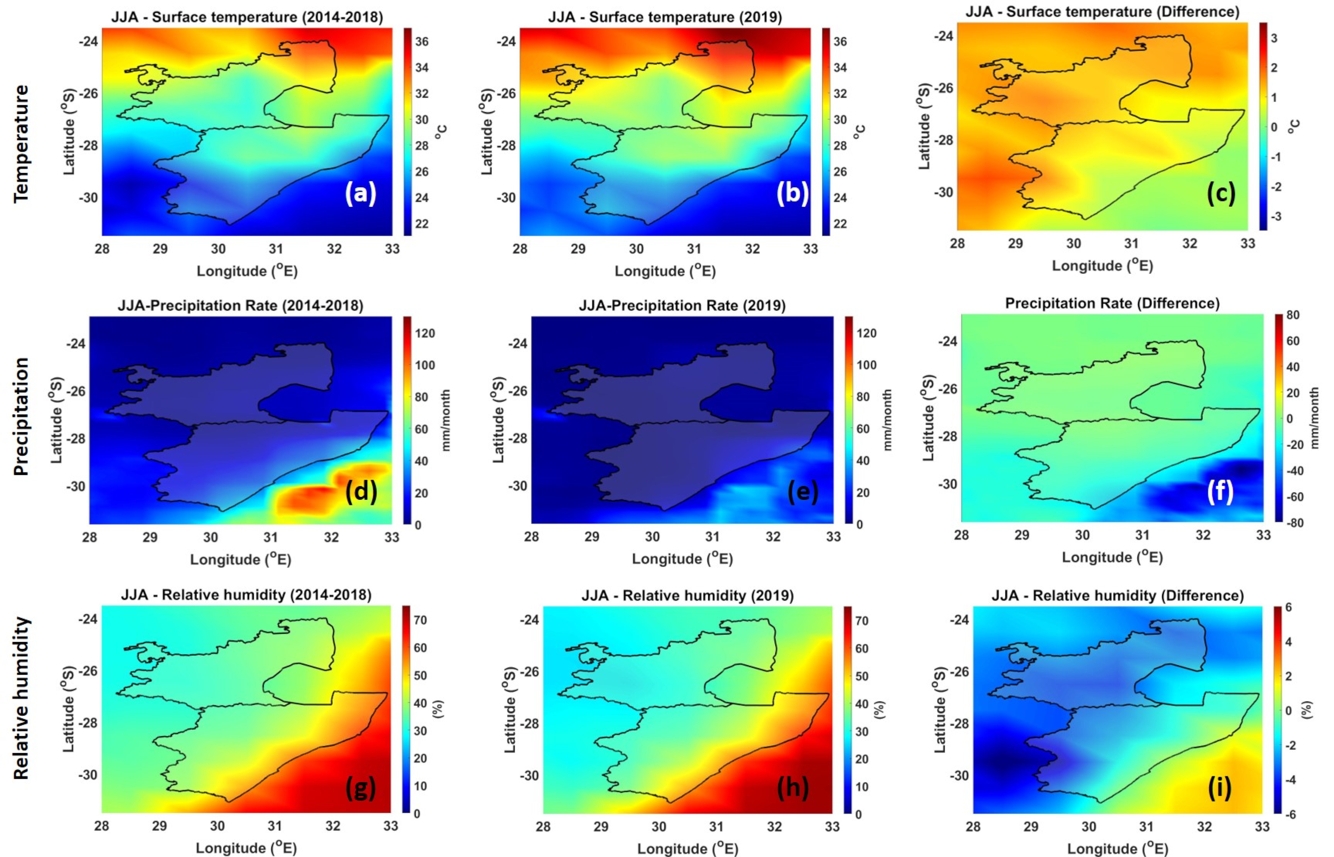
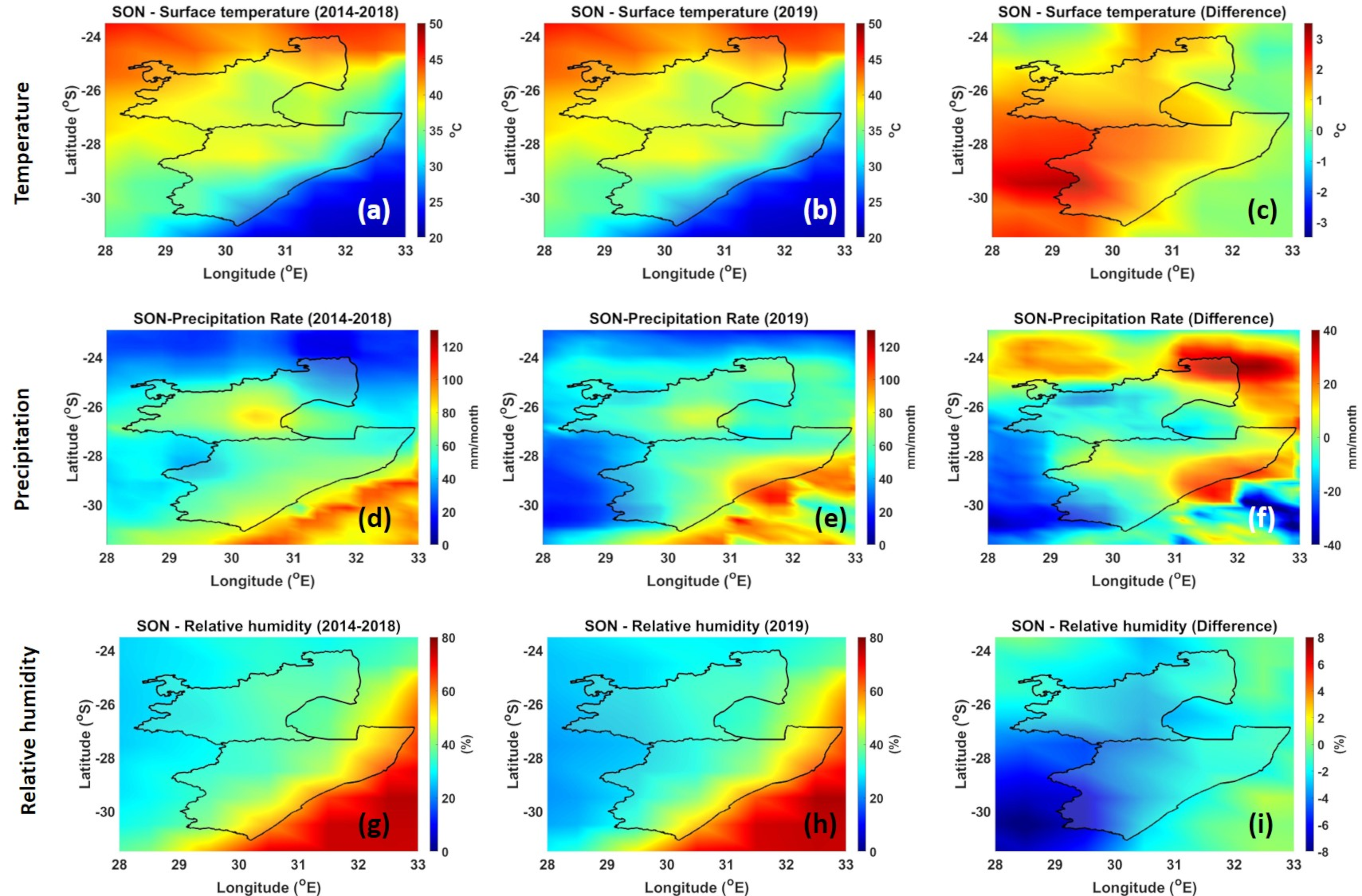
4.2. Meteorological Conditions
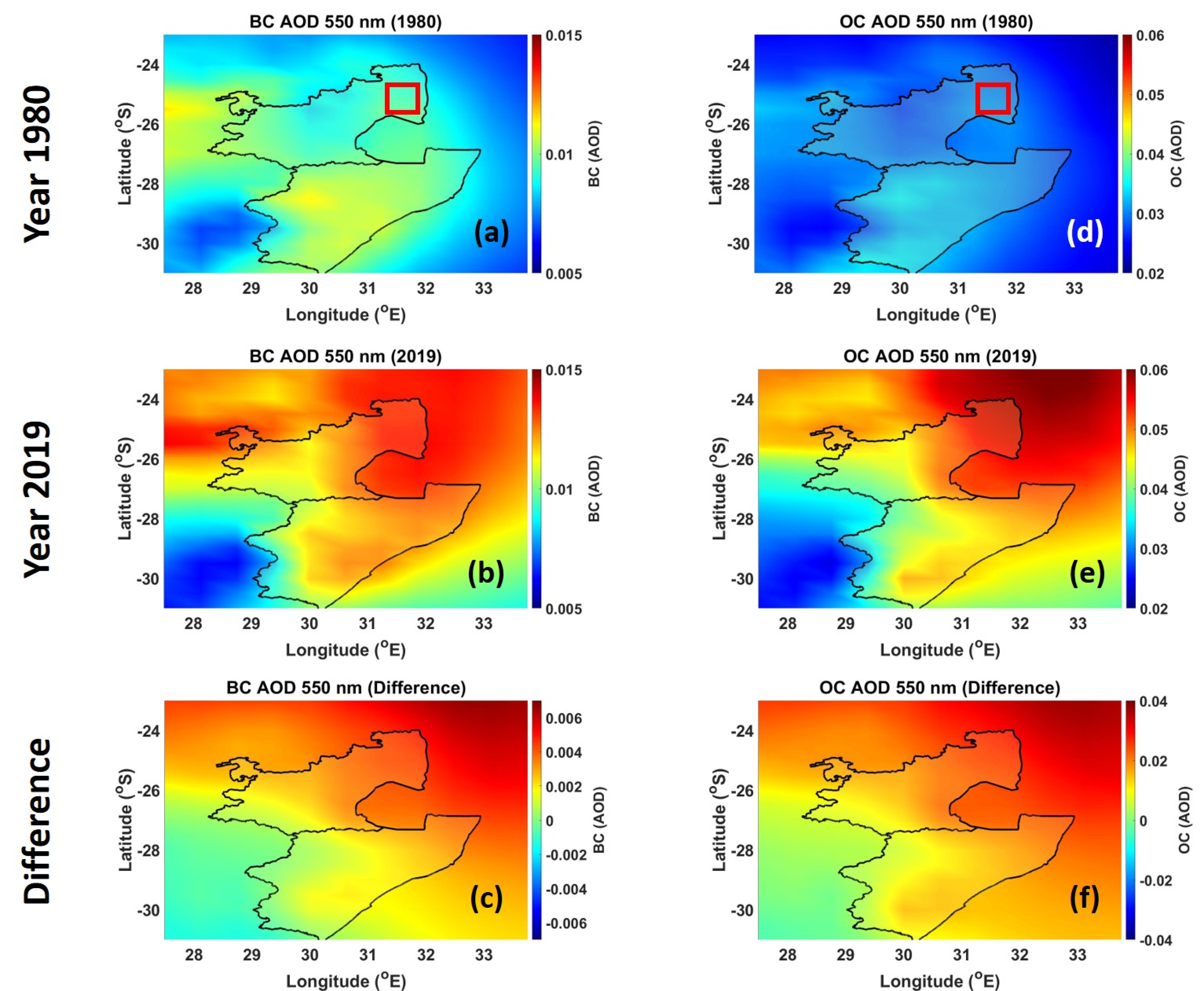
4.3. Trend Analysis and Dispersion of Pollutants
4.3.1. Emissions from Sugarcane Burning
4.3.2. Rainfall Trends
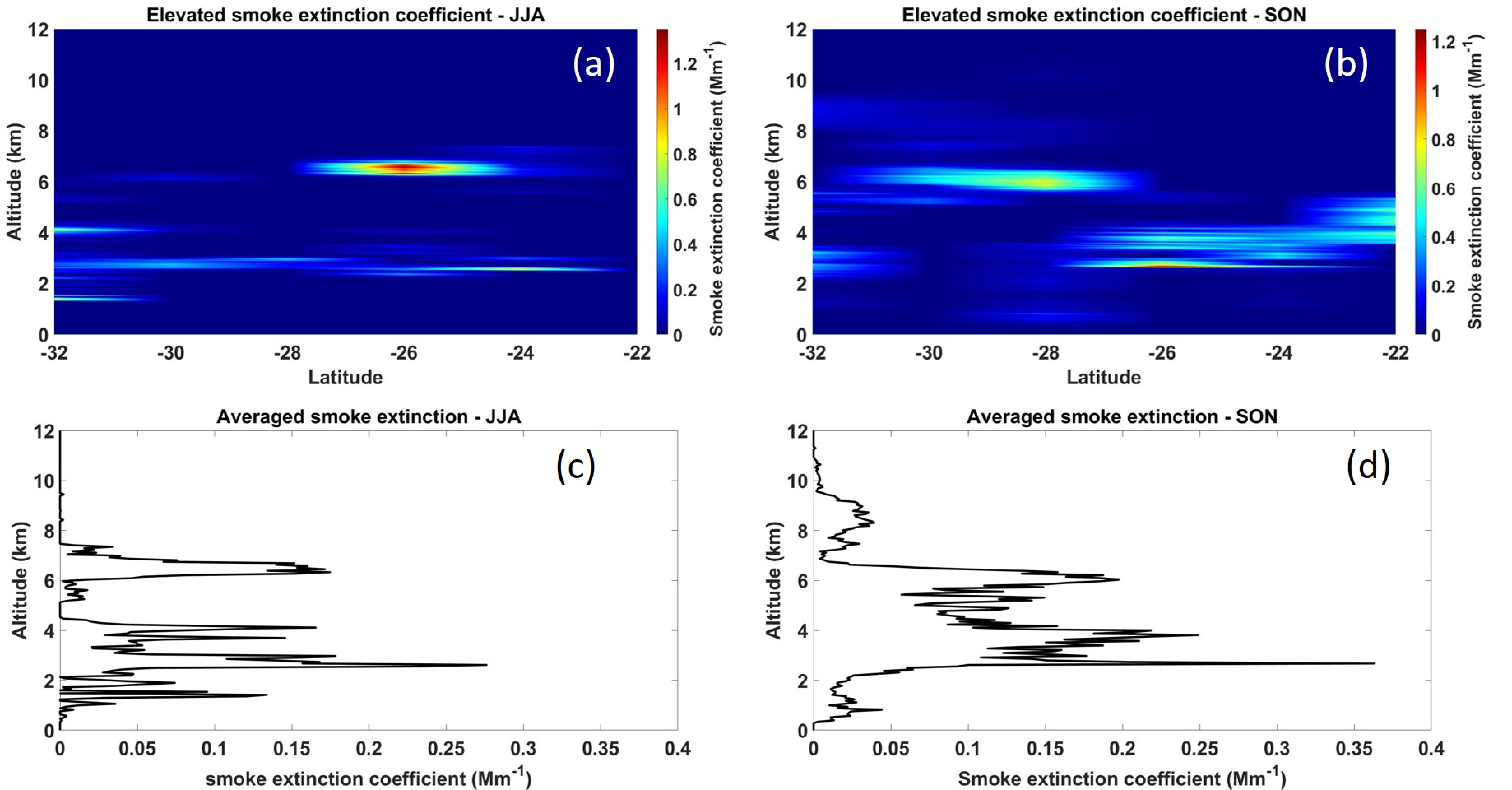
4.4. Dispersion and Transport of Pollutants
5. Conclusions
Author Contributions
Funding
Institutional Review Board Statement
Informed Consent Statement
Data Availability Statement
Acknowledgments
Conflicts of Interest
References
- Mintz, S.W. Sweetness and Power: The Place of Sugar in Modern History; Penguin Books: New York, NY, USA, 1985. [Google Scholar]
- Van der Poel, P.W.; Schiweck, H.; Schwartz, T. Sugar Technology Beet and Cane Sugar Manufacture. Verlag Dr. Albert Bartens KG: Berlin, Germany, 1998; pp. 479–563. [Google Scholar]
- Total Sugar Production Worldwide from 2009/2010 to 2020/2021 (in Million Metric Tons). Available online: https://www.statista.com/statistics/249679/total-production-of-sugar-worldwide/ (accessed on 16 April 2021).
- Hess, T.M.; Sumberg, J.; Biggs, T.; Georgescu, M.; Haro-Monteagudo, D.; Jewitt, G.; Ozdogan, M.; Marshall, M.; Thenkabail, P.; Daccache, A.; et al. A sweet deal? Sugarcane, water and agricultural transformation in Sub-Saharan Africa. Glob. Environ. Chang. 2016, 39, 181–194. [Google Scholar] [CrossRef] [Green Version]
- Guidelines for Burning Sugarcane. Available online: https://sasri.org.za/storage/Information_Sheets/IS_4.8-Guidelines-for-burning-sugarcane.pdf (accessed on 16 April 2021).
- Why We Burn. Available online: https://northcoastcourier.co.za/10604/burn/ (accessed on 16 April 2021).
- Artaxo, P.; Oyola, P.; Martinez, R. Aerosol composition and source apportionment in Santiago de Chile. Nucl. Instrum. Methods Phys. Res. B 1999, 150, 409–416. [Google Scholar] [CrossRef]
- Crutzen, P.J.; Andreae, M.O. Biomass burning in the tropics: Impact on atmospheric chemistry and biogeochemical cycles. Science 1990, 250, 1669–1678. [Google Scholar] [CrossRef]
- Andreae, M.O.; Artaxo, P.; Fischer, H.; Freitas, S.R.; Gregoire, J.-M.; Hansel, A.; Hoor, P.; Kormann, R.; Krejci, R.; Lange, L.; et al. Transport of biomass burning smoke to the upper troposphere by deep convection in the equatorial region. Geophys. Res. Lett. 2001, 28, 951–954. [Google Scholar] [CrossRef] [Green Version]
- Bond, T.C.; Streets, D.G.; Yarber, K.F.; Nelson, S.M.; Woo, J.-H.; Klimont, Z. A technology-based global inventory of black and organic carbon emissions from combustion. J. Geophys. Res. 2004, 109, D14203. [Google Scholar] [CrossRef] [Green Version]
- Guenther, A.; Karl, T.; Harley, P.; Wiedinmyer, C.; Palmer, P.I.; Geron, C. Estimates of global terrestrial isoprene emissions using MEGAN (Model of Emissions of Gases and Aerosols from Nature). Atmos. Chem. Phys. 2006, 6, 3181–3210. [Google Scholar] [CrossRef] [Green Version]
- Sudo, K.; Akimoto, H. Global source attribution of tropospheric ozone: Long range transport from various source regions. J. Geophys. Res. 2007, 112, D12302. [Google Scholar] [CrossRef]
- Akagi, S.K.; Yokelson, R.J.; Wiedinmyer, C.; Alvarado, M.J.; Reid, S.J.; Karl, T.; Crounse, J.D.; Wennberg, P.O. Emission factors for open and domestic biomass burning for use in atmospheric models. Atmos. Chem. Phys. 2011, 11, 4039–4072. [Google Scholar] [CrossRef] [Green Version]
- Sigsgaard, T.; Forsberg, B.; Annesi-Maesano, I.; Blomberg, A.; Bølling, A.; Boman, C.; Bønløkke, J.; Brauer, M.; Bruce, N.; Héroux, M.-E.; et al. Health impacts of anthropogenic biomass burning in the developed world. Eur. Respir. J. 2015, 46, 1577–1588. [Google Scholar] [CrossRef] [Green Version]
- Ballesteros-González, K.; Sullivan, A.P.; Morales-Betancourt, R. Estimating the air quality and health impacts of biomass burning in northern South America using a chemical transport model. Sci. Total Environ. 2020, 739, 139755. [Google Scholar] [CrossRef]
- Chen, J.; Li, C.; Ristovski, Z.; Milic, A.; Gu, Y.; Islam, M.S.; Wang, S.; Hao, J.; Zhang, H.; He, C.; et al. A review of biomass burning: Emissions and impacts on air quality, health and climate in China. Sci. Total Environ. 2020, 579, 1000–1034. [Google Scholar] [CrossRef] [Green Version]
- Jacobson, M.Z. Effects of biomass burning on climate, accounting for heat and moisture fluxes, black and brown carbon, and cloud absorption effects. J. Geophys. Res. Atmos. 2014, 119, 8980–9002. [Google Scholar] [CrossRef]
- Kaufman, Y.J.; Fraser, R.S.; Mahoney, R.L. Fossil fuel and biomass burning effect on climate—Heating or cooling? J. Clim. 1991, 4, 578–588. [Google Scholar] [CrossRef] [Green Version]
- Andreae, M. Biomass burning in the tropics: Impact on environmental quality and global climate. Popul. Dev. Rev. 1990, 16, 268–291. [Google Scholar] [CrossRef]
- Mashoko, L.; Mbohwa, C.; Thomas, V.M. LCA of the South African sugar industry. J. Environ. Plan. Manag. 2010, 53, 793–807. [Google Scholar] [CrossRef]
- Pryor, S.W.; Smithers, J.; Lyne, P.; van Antwerpen, R. Impact of agricultural practices on energy use and greenhouse gas emissions for South African sugarcane production. J. Clean. Prod. 2017, 141, 137–145. [Google Scholar] [CrossRef] [Green Version]
- Eustice, T.; Van Der Laan, M.; Van Antwerpen, R. Comparison of greenhouse gas emissions from trashed and burnt sugarcane cropping systems in South Africa. In Proceedings of the 84th Annual Congress-South African Sugar Technologists’ Association, Durban, South Africa, 17–19 August 2011; pp. 326–339. [Google Scholar]
- SASA. Sugar Industry Statistical Information. Available online: https://sasa.org.za/facts-and-figures/ (accessed on 21 April 2021).
- Parker, W.S. Reanalyses and observations: What’s the difference? Bull. Am. Meteorol. Soc. 2016, 97, 1565–1572. [Google Scholar] [CrossRef] [Green Version]
- Rienecker, M.M.; Suarez, M.J.; Gelaro, R.; Todling, R.; Bacmeister, J.; Liu, E.; Bosilovich, M.G.; Schubert, S.D.; Takacs, L.; Kim, G.; et al. MERRA: NASA’s modern-era retrospective analysis for research and applications. J. Clim. 2011, 24, 3624–3648. [Google Scholar] [CrossRef]
- Gelaro, R.; McCarty, W.; Suárez, M.J.; Todling, R.; Molod, A.; Takacs, L.; Randles, C.A.; Darmenov, A.; Bosilovich, M.G.; Reichle, R.; et al. The modern-era retrospective analysis for research and applications, Version 2 (MERRA-2). J. Clim. 2017, 30, 5419–5454. [Google Scholar] [CrossRef]
- Molod, A.; Takacs, L.; Suarez, M.; Bacmeister, J. Development of the GEOS-5 atmospheric general circulation model: Evolution from MERRA to MERRA2. Geosci. Model. Dev. 2015, 8, 1339–1356. [Google Scholar] [CrossRef] [Green Version]
- Rienecker, M.; Suarez, M.; Todling, R.; Bacmeister, J.; Takacs, L.; Liu, H.-C.; Gu, W.; Sienkiewicz, M.; Koster, R.; Gelaro, R. The GEOS-5 Data Assimilation System—Documentation of Versions 5.0.1, 5.1.0, and 5.2.0; Technical Report Series on Global Modeling and Data Assimilation; NASA: Washington, DC, USA, 2008. [Google Scholar]
- Randles, C.A.; da Silva, A.M.; Buchard, V.; Colarco, P.R.; Darmenov, A.; Govindaraju, R.; Smirnov, A.; Holben, B.; Ferrare, R.; Hair, J.; et al. The MERRA-2 aerosol reanalysis, 1980 onward. Part I: System description and data as-similation evaluation. J. Clim. 2017, 30, 6823–6850. [Google Scholar] [CrossRef]
- Buchard, V.; Randles, C.A.; da Silva, A.M.; Darmenov, A.; Colarco, P.R.; Govindaraju, R.; Ferrare, R.; Hair, J.; Beyersdorf, A.J.; Ziemba, L.D.; et al. The MERRA-2 aerosol reanalysis, 1980 onward. Part II: Evaluation and case studies. J. Clim. 2017, 30, 6851–6872. [Google Scholar] [CrossRef]
- Putman, W.; Lin, S.-J. Finite volume transport on various cubed sphere grids. J. Comput. Phys. 2007, 227, 55–78. [Google Scholar] [CrossRef]
- Bloom, S.; Takacs, L.; DaSilva, A.; Ledvina, D. Data assimilation using incremental analysis updates. Mon. Weather Rev. 1996, 124, 1256–1271. [Google Scholar] [CrossRef] [Green Version]
- Stephens, G.L.; Vane, D.G.; Boain, R.J.; Mace, G.G.; Sassen, K.; Wang, Z.; Illingworth, A.J.; O’Connor, E.J.; Rossow, W.B.; Durden, S.L.; et al. The CloudSat mission and the A-Train: A new dimension of space-based observations of clouds and precipitation. Bull. Am. Meteor. Soc. 2002, 83, 1771–1790. [Google Scholar] [CrossRef] [Green Version]
- Winker, D.M.; Pelon, J.; McCormick, M.P. The CALIPSO Mission: Spaceborne Lidar for Observation of Aerosols and Clouds. In Lidar Remote Sensing for Industry and Environment Monitoring III; Singh, U.N., Itabe, T., Lui, Z., Eds.; SPIE: Bellingham, WA, USA, 2003; Volume 4893, pp. 1–11. [Google Scholar]
- Winker, D.M.; Vaughan, M.A.; Omar, A.; Hu, Y.; Powell, K.A.; Liu, Z.; Hunt, W.H.; Young, S.A. Overview of the CALIPSO mission and CALIOP data processing algorithms. J. Atmos. Ocean. Technol. 2009, 26, 2310–2323. [Google Scholar] [CrossRef]
- Omar, A.H.; Winker, D.M.; Vaughan, M.A.; Hu, Y.; Trepte, C.R.; Ferrare, R.A.; Lee, K.; Hostetler, C.A.; Kittaka, C.; Rogers, R.R.; et al. The CALIPSO automated aerosol classification and lidar ratio selection algorithm. J. Atmos. Ocean. Technol. 2009, 26, 1994–2014. [Google Scholar] [CrossRef]
- Winker, D.M.; Pelon, J.; Coakley, J.A., Jr.; Ackerman, S.A.; Charlson, R.J.; Colarco, P.R.; Flamant, P.; Fu, Q.; Hoff, R.M.; Kittaka, C.; et al. The CALIPSO mission: A global 3D view of aerosols and clouds. Bull. Am. Meteorol. Soc. 2010, 91, 1211–1229. [Google Scholar] [CrossRef]
- Hartmut, H.; Aumann, H.; Miller, C.R. Atmospheric infrared sounder (AIRS) on the earth observing system. In Advanced and Next-Generation Satellites; SPIE: Bellingham, WA, USA, 1995; Volume 2583. [Google Scholar]
- Chahine, M.T.; Pagano, T.; Aumann, H.; Atlas, R.; Barnet, C.; Blaisdell, J.; Chen, L.; Divakarla, M.; Fetzer, E.; Goldberg, M.; et al. AIRS: Improving weather forecasting and providing new data on greenhouse gases. Bull. Am. Meteorol. Soc. 2006, 87, 911–926. [Google Scholar] [CrossRef] [Green Version]
- Menzel, W.P.; Schmit, T.J.; Zhang, P.; Li, J. Satellite-based atmospheric infrared sounder development and applications. Bull. Am. Meteorol. Soc. 2018, 99, 583–603. [Google Scholar] [CrossRef]
- Kummerow, C.; Simpson, J.; Thiele, O.; Barnes, W.; Chang, A.T.C.; Stocker, E.; Adler, R.F.; Hou, A.; Kakar, R.; Wentz, F.; et al. The status of the tropical rainfall measuring mission (TRMM) after two years in orbit. J. Appl. Meteorol. 2000, 39, 1965–1982. [Google Scholar] [CrossRef]
- Liu, Z.; Ostrenga, D.; Teng, W.; Kempler, S. Tropical rainfall measuring mission (TRMM) precipitation data and services for research and applications. Bull. Am. Meteorol. Soc. 2012, 93, 1317–1325. [Google Scholar] [CrossRef] [Green Version]
- Draxler, R.R.; Hess, G.D. An overview of the HYSPLIT_4 modeling system for trajectories, dispersion, and deposition. Aust. Meteor. Mag. 1998, 47, 295–308. [Google Scholar]
- Fleming, Z.L.; Monks, P.S.; Manning, A.J. Review: Untangling the influence of air-mass history in interpreting observed atmospheric composition. Atmos. Res. 2012, 104, 1–39. [Google Scholar] [CrossRef] [Green Version]
- Rolph, G.; Stein, A.; Stunder, B. Real-time environmental applications and display sYstem: READY. Environ. Model. Softw. 2017, 95, 210–228. [Google Scholar] [CrossRef]
- Stein, A.F.; Draxler, R.R.; Rolph, G.D.; Stunder, B.J.B.; Cohen, M.D.; Ngan, F. NOAA’s HYSPLIT atmospheric transport and dispersion modeling system. Bull. Am. Meteorol. Soc. 2015, 96, 2059–2077. [Google Scholar] [CrossRef]
- Shikwambana, L.; Sivakumar, V. Long-range transport of volcanic aerosols over South Africa: A case study of the Calbuco volcanic eruption in Chile during April 2015. S. Afr. Geogr. J. 2018, 100, 349–363. [Google Scholar] [CrossRef]
- Shikwambana, L.; Ncipha, X.; Malahlela, O.E.; Mbatha, N.; Sivakumar, V. Characterisation of aerosol constituents from wildfires using satellites and model data: A case study in Knysna, South Africa. Int. J. Remote Sens. 2019, 40, 4743–4761. [Google Scholar] [CrossRef]
- Sneyers, R. On the Statistical Analysis of Series of Observations; Technical Note, No. 143; World Meteorological Organization (WMO): Geneva, Switzerland, 1990. [Google Scholar]
- Sneyers, R. Climate chaotic instability: Statistical determination and theoretical background. Environmetrics 1997, 8, 517–532. [Google Scholar] [CrossRef]
- Sneyers, R.; Tuomenvirta, H.; Heino, R. Observations inhomogeneities and detection of climate change the case of the Oulu (Finland) air temperature series. Geophysica 1998, 34, 159–178. [Google Scholar]
- Mosmann, V.; Castro, A.; Fraile, R.; Dessens, J.; Sanchez, J. Detection of statistically significant trends in the summer precipitation of mainland Spain. Atmos. Res. 2004, 70, 43–53. [Google Scholar] [CrossRef]
- James, P.; Woodhouse, P. Crisis and differentiation among small-scale sugar cane growers in Nkomazi, South Africa. J. S. Afr. Stud. 2017, 43, 535–549. [Google Scholar] [CrossRef] [Green Version]
- Jacobson, M.Z.; Kaufman, Y.J. Wind reduction by aerosol particles. Geophys. Res. Lett. 2006, 33, L24814. [Google Scholar] [CrossRef] [Green Version]
- Liu, C.; Huang, J.; Fedorovich, E.; Hu, X.-M.; Wang, Y.; Lee, X. The effect of aerosol radiative heating on turbulence statistics and spectra in the atmospheric convective boundary layer: A large-eddy simulation study. Atmosphere 2018, 9, 347. [Google Scholar] [CrossRef] [Green Version]
- Benson, R.P.; Roads, J.O.; Weise, D.R. Climatic and weather factors affecting fire occurrence and behavior. In Wildland Fires and Air Pollution. Developments in Environmental Science, 1st ed; Bytnerowicz, A., Arbaugh, M., Andersen, C., Riebau, A., Eds.; Elsevier: Amsterdam, The Netherlands, 2009; Volume 8, pp. 37–60. [Google Scholar]
- Shikwambana, L.; Mhangara, P.; Mbatha, N. Trend analysis and first time observations of sulphur dioxide and nitrogen dioxide in South Africa using TROPOMI/Sentinel-5P data. Int. J. Appl. Earth Obs. 2020, 9, 102130. [Google Scholar] [CrossRef]
- Kruger, A.C.; Retief, J.V.; Goliger, A.M. Strong winds in South Africa: Part 2 Mapping of updated statistics. J. S. Afr. Inst. Civ. Eng. 2013, 55, 46–58. [Google Scholar]
- Myers, A.; Fig, D.; Tugendhaft, A.; Myers, J.E.; Hofman, K.J. The history of the South African sugar industry illuminates deeply rooted obstacles for sugar reduction anti-obesity interventions. Afr. Stud. 2017, 76, 475–490. [Google Scholar] [CrossRef]
- Census of Commercial Agriculture. 2017. Available online: http://www.statssa.gov.za/publications/Report-11-02-01/Report-11-02-012017.pdf (accessed on 24 May 2021).
- Cooke, W.F.; Liousse, C.; Cachier, H.; Feichter, J. Construction of a 1 degrees x 1 degrees fossil fuel emission data set for carbonaceous aerosol and implementation and radiative impact in the ECHAM4 model. J. Geophys. Res. 1999, 104, 22137–22162. [Google Scholar] [CrossRef]
- Kanakidou, M.; Seinfeld, J.H.; Pandis, S.N.; Barnes, I.; Dentener, F.J.; Facchini, M.C.; Van Dingenen, R.; Nenes, B.A.; Nielsen, C.J.; Swietlicki, E.; et al. Organic aerosol and global climate modelling: A review. Atmos. Chem. Phys. 2005, 5, 1053–1123. [Google Scholar] [CrossRef] [Green Version]
- Malik, S.D.; Tomar, B.S. Impact of rainfall and temperature on sugarcane quality. Agric. Sci. Digest. 2003, 23, 50–52. [Google Scholar]
- Chandiposha, M. Potential impact of climate change in sugarcane and mitigation strategies in Zimbabwe. Afr. J. Agric. Res. 2013, 8, 2814–2818. [Google Scholar]
- Basnayake, J.; Jackson, P.A.N.; Inman-Bamber, G.; Lakshmanan, P. Sugarcane for water-limited environments: Genetic variation in cane yield and sugar content in response to water stress. S. Afr. J. Bot. 2012, 63, 6023–6033. [Google Scholar] [CrossRef] [PubMed]
- Hussain, S.; Khaliq, A.; Mehmood, U.; Qadir, T.; Saqib, M.; Iqbal, M.A.; Hussain, S. Sugarcane production under changing climate: Effects of environmental vulnerabilities on sugarcane diseases, insects and weeds. In Climate Change and Agriculture; IntechOpen: London, UK, 2018. [Google Scholar]
- Mbatha, N.; Xulu, S. Time series analysis of MODIS-derived NDVI for the Hluhluwe-Imfolozi park, South Africa: Impact of recent intense drought. Climate 2018, 6, 95. [Google Scholar] [CrossRef] [Green Version]
- Shikwambana, L.; Kganyago, M. Observations of emissions and the influence of meteorological conditions during wildfires: A case study in the USA, Brazil, and Australia during the 2018/19 period. Atmosphere 2021, 12, 11. [Google Scholar] [CrossRef]
- WHO. Health Effects of Black Carbon. Available online: https://www.euro.who.int/__data/assets/pdf_file/0004/162535/e96541.pdf (accessed on 10 June 2021).
- Solomon, S.; Plattner, G.-K.; Knutti, R.; Friedlingstein, P. Irreversible climate change due to carbon dioxide emissions. Proc. Natl. Acad. Sci. USA 2009, 106, 1704–1709. [Google Scholar] [CrossRef] [Green Version]


| Mpumalanga Province | KwaZulu Natal Province | |||
|---|---|---|---|---|
| Parameter | JJA Season | SON Season | JJA Season | SON Season |
| Temperature (°C) | 31 | 38 | 25 | 28 |
| Precipitation (mm/month) | 0 | 50 | 0 | 80 |
| Relative humidity (%) | 50 | 52 | 60 | 52 |
| Wind speed (m·s−1) and direction | 6.5 (north-easterly) | 6.5 (westerly) | 7–8 (south-westerly) | 7–8 (westerly) |
Publisher’s Note: MDPI stays neutral with regard to jurisdictional claims in published maps and institutional affiliations. |
© 2021 by the authors. Licensee MDPI, Basel, Switzerland. This article is an open access article distributed under the terms and conditions of the Creative Commons Attribution (CC BY) license (https://creativecommons.org/licenses/by/4.0/).
Share and Cite
Shikwambana, L.; Ncipha, X.; Sangeetha, S.K.; Sivakumar, V.; Mhangara, P. Qualitative Study on the Observations of Emissions, Transport, and the Influence of Climatic Factors from Sugarcane Burning: A South African Perspective. Int. J. Environ. Res. Public Health 2021, 18, 7672. https://doi.org/10.3390/ijerph18147672
Shikwambana L, Ncipha X, Sangeetha SK, Sivakumar V, Mhangara P. Qualitative Study on the Observations of Emissions, Transport, and the Influence of Climatic Factors from Sugarcane Burning: A South African Perspective. International Journal of Environmental Research and Public Health. 2021; 18(14):7672. https://doi.org/10.3390/ijerph18147672
Chicago/Turabian StyleShikwambana, Lerato, Xolile Ncipha, Sivakumar Kandasami Sangeetha, Venkataraman Sivakumar, and Paidamwoyo Mhangara. 2021. "Qualitative Study on the Observations of Emissions, Transport, and the Influence of Climatic Factors from Sugarcane Burning: A South African Perspective" International Journal of Environmental Research and Public Health 18, no. 14: 7672. https://doi.org/10.3390/ijerph18147672