1. Introduction
This work explores the interplay among Wilson–Cowan models, connection matrices, and non-Archimedean models of complex systems.
The Wilson–Cowan model describes the evolution of excitatory and inhibitory activity in a synaptically coupled neuronal network. The model is given by the following system of non-linear integro-differential evolution equations:
where
is a temporal coarse-grained variable describing the proportion of excitatory neuron firing per unit of time at position
at instant
. Similarly, the variable
represents the activity of the inhibitory population of neurons. The main parameters of the model are the strength of the connections among the subtypes of population (
,
,
, and
) and the strength of the input to each subpopulation (
and
). This model generates a diversity of dynamical behaviors that are representative of activity observed in the brain, such as multistability, oscillations, traveling waves, and spatial patterns; see, e.g., [
1,
2,
3] and the references therein.
We formulate the Wilson–Cowan model on locally compact Abelian topological groups. The classical model corresponds to the group
. In this framework, using classical techniques on semilinear evolution equations (see, e.g., [
4,
5]), we show that the corresponding Cauchy problem is locally well posed, and if
, it is globally well posed; see Theorem 1. This last condition corresponds to the case of two coupled perceptrons.
Nowadays, there is a large number of experimental data about the connection matrices of the cerebral cortex of invertebrates and mammalians. Based on these data, several researchers hypothesized that cortical neural networks are arranged in fractal or self-similar patterns and have the small-world property; see, e.g., [
6,
7,
8,
9,
10,
11,
12,
13,
14,
15,
16,
17,
18,
19] and the references therein. Connection matrices provide a static view of neural connections.
The investigation of the relationships between the Wilson–Cowan model and connection matrices is quite natural, since the model was proposed to explain the cortical dynamics, while the matrices describe the functional geometry of the cortex. We initiate this study here.
A network having the small-world property necessarily has long-range interactions; see
Section 3. In the Wilson–Cowan model, the kernels (
,
,
, and
) describing the neural interactions are Gaussian in nature, so only short-range interactions may occur. For practical purposes, these kernels have compact support. On the other hand, the Wilson–Cowan model on a general group requires that the kernels be integrable; see
Section 2. We argue that
G must be compact to satisfy the small-world property. Under this condition, any continuous kernel is integrable. Wilson and Cowan formulated their model on the group
. The only compact subgroup of this group is the trivial one. The small-world property is, therefore, incompatible with the classical Wilson–Cowan model.
It is worth noting that the absence of non-trivial compact subgroups in
is a consequence of the Archimedean axiom (the absolute value is not bounded on the integers). Therefore, to avoid this problem, we can replace
with a non-Archimedean field, which is a field where the Archimedean axiom is not valid. We selected the field of the
p-adic numbers. This field has infinitely many compact subgroups, and the balls have center in the origin. We selected the unit ball, the ring of
p-adic numbers
. The
p-adic integers are organized in an infinite rooted tree. We used this hierarchical structure as the topology for our
p-adic version of the Wilson–Cowan model. In principle, we could use other groups, such as the classical compact groups, to replace
, but it is also essential to have a rigorous study of the discretization of the model. For the group
, this task can be performed using standard approximation techniques for evolutionary equations; see, e.g., [
5] (Section 5.4).
The p-adic Wilson–Cowan model admits good discretizations. Each discretization corresponds to a system of non-linear integro-differential equations on a finite rooted tree. We show that the solution of the Cauchy problem of this discrete system provides a good approximation to the solution of the Cauchy problem of the p-adic Wilson–Cowan model; see Theorem 2.
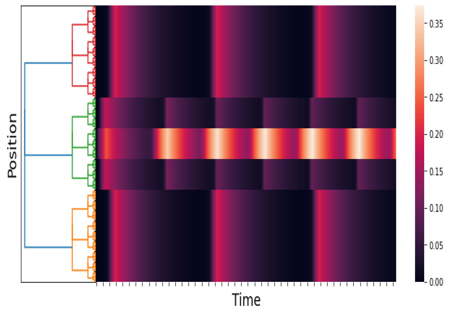
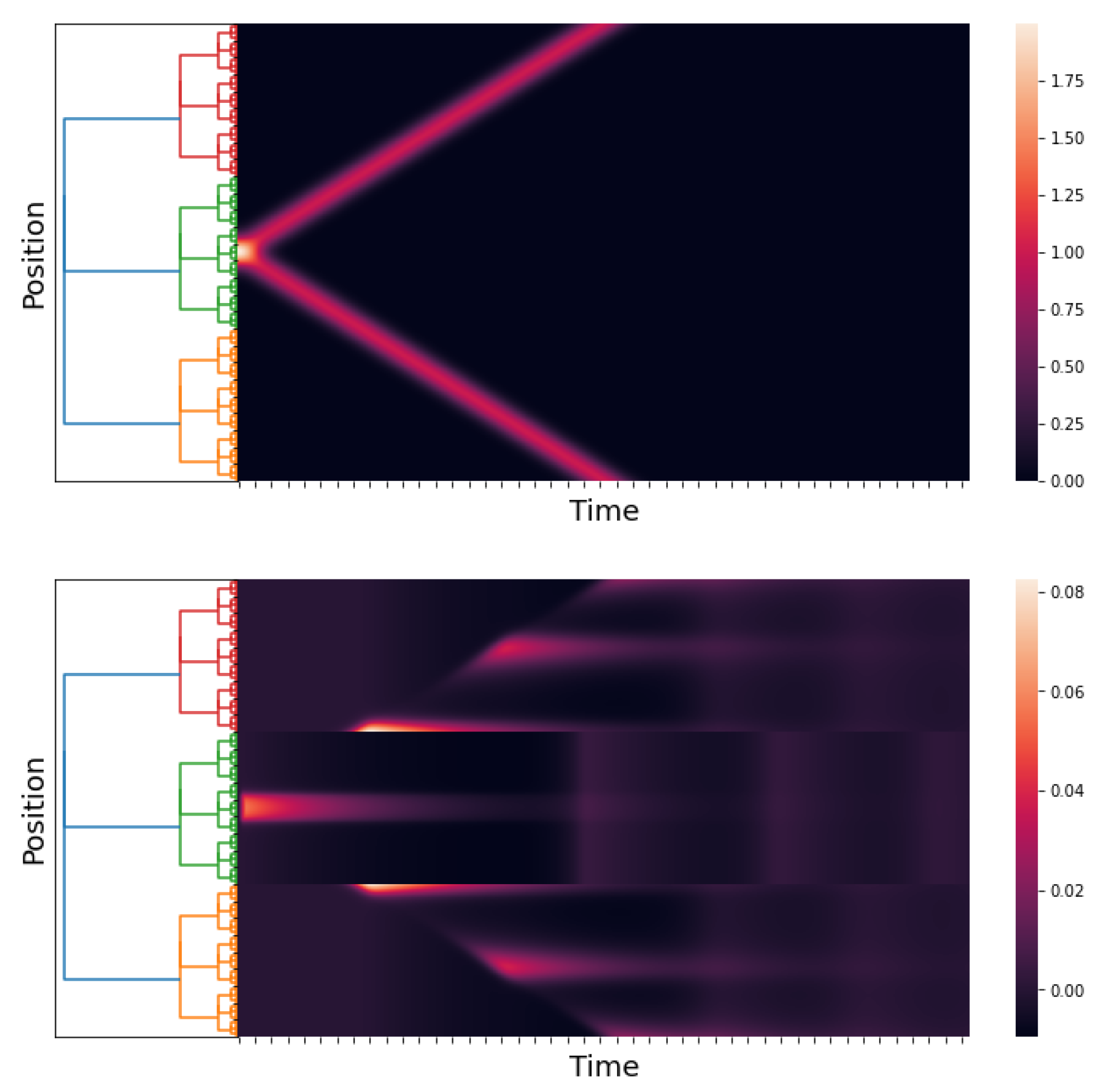
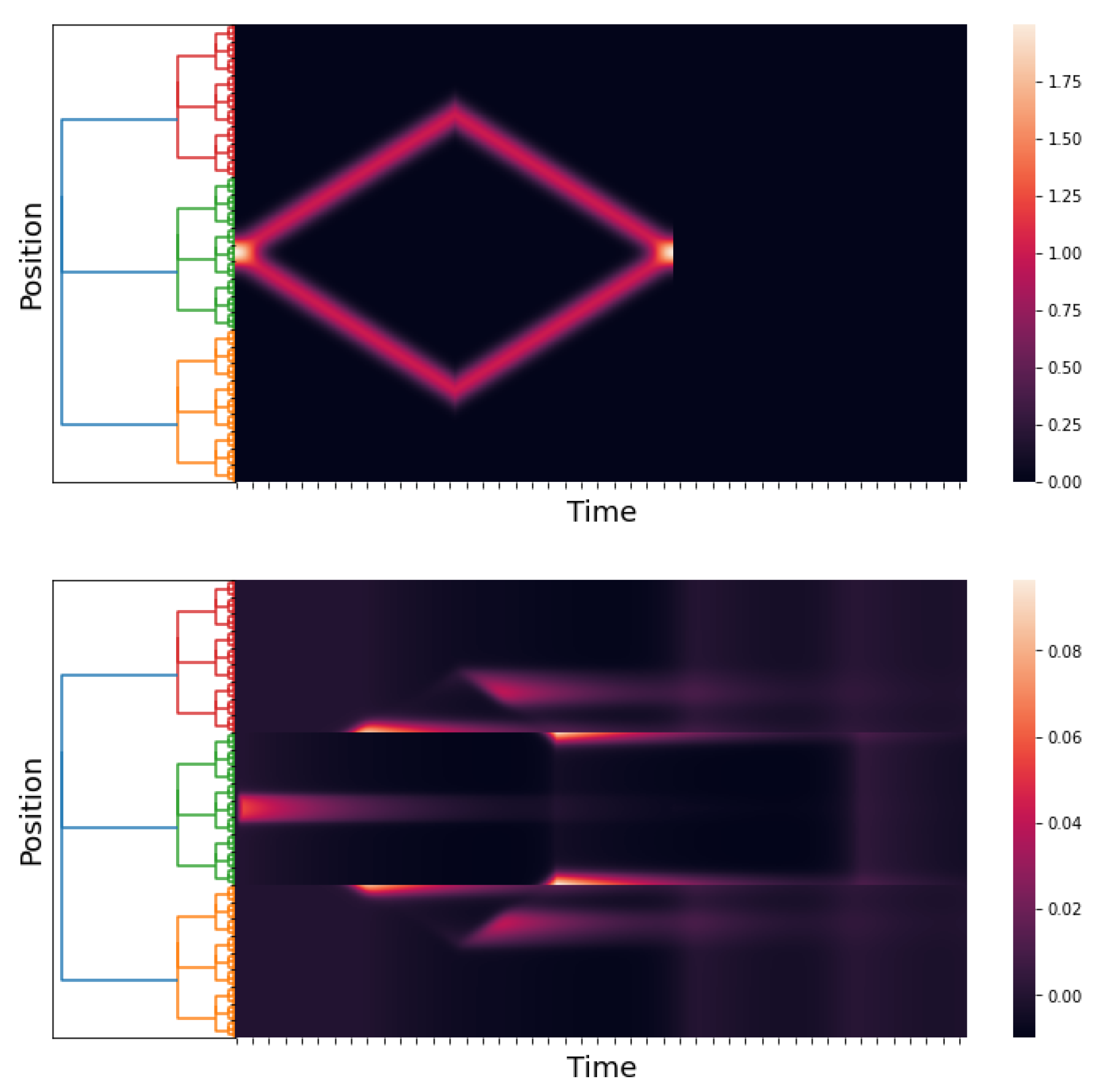
We provide extensive numerical simulations of
p-adic Wilson–Cowan models. In
Section 5, we present three numerical simulations showing that the
p-adic models provide a similar explanation to the numerical experiments presented in [
2]. In these experiments, the kernels (
,
,
, and
) were chosen to have properties similar to those of the kernels used in [
2]. In
Section 6, we consider the problem of how to integrate the connection matrices into the
p-adic Wilson–Cowan model. This fundamental scientific task aims to use the vast number of data on maps of neural connections to understand the dynamics of the cerebral cortex of invertebrates and mammalians. We show that the connection matrix of the cat cortex can be well approximated with a
p-adic kernel
. We then replace the excitatory–excitatory relation term
with
but keep the other kernels as in Simulation 1 presented in
Section 5. The response of this network is entirely different from that given in Simulation 1. For the same stimulus, the response of the last network exhibits very complex patterns, while the response of the network presented in Simulation 1 is simpler.
The
p-adic analysis has shown to be the right tool in the construction of a wide variety of models of complex hierarchic systems; see, e.g., [
20,
21,
22,
23,
24,
25,
26,
27,
28] and the references therein. Many of these models involve abstract evolution equations of the type
. In these models, the discretization of operator
is an ultrametric matrix
, where
is a finite rooted tree with
l levels and
branches; here,
p is a fixed prime number (see the numerical simulations in [
27,
28]). Locally, connection matrices look very similar to matrices
. The problem of approximating large connection matrices with ultrametric matrices is an open problem.
4. -Adic Wilson–Cowan Models
The previous section shows that the classical Wilson–Cowan can be formulated on a large class of topological groups. This formulation does not use any information about the geometry of the neural interaction, which is encoded in the geometry of the group . The next step is to incorporate the connection matrices into the Wilson–Cowan model, which requires selecting a specific group. In this section, we propose the p-adic Wilson–Cowan models where is the ring of p-adic integers .
4.1. The p-Adic Integers
This section reviews some basic results of
p-adic analysis required in this article. For a detailed exposition on
p-adic analysis, the reader may consult [
29,
30,
31,
32]. For a quick review of
p-adic analysis, the reader may consult [
33].
From now on,
p denotes a fixed prime number. The ring of
p-adic integers
is defined as the completion of the ring of integers
with respect to the
p-adic norm
, which is defined as
where
a is an integer coprime with
p. The integer
, with
, is called the
p-
adic order of
x.
Any non-zero
p-adic integer
x has a unique expansion of the form
with
, where
k is a non-negative integer, and
are numbers from the set
. There are natural field operations, sum and multiplication, on
p-adic integers; see, e.g., [
34]. Norm (
15) extends to
as
for a non-zero
p-adic integer
x.
The metric space
is a complete ultrametric space. Ultrametric means that
. As a topological space,
is homeomorphic to a Cantor-like subset of the real line; see, e.g., [
29,
30,
35].
For , let us denote by the ball of radius with center in and take . Ball equals the ring ofp-adic integers . We use to denote the characteristic function of ball . Given two balls in , either they are disjoint, or one is contained in the other. The balls are compact subsets; thus, is a compact topological space.
Tree-like Structures
The set of
p-adic integers modulo
,
, consists of all the integers of the form
. These numbers form a complete set of representatives of the elements of additive group
, which is isomorphic to the set of integers
(written in base
p) modulo
. By restricting
to
, it becomes a normed space, and
. With the metric induced by
,
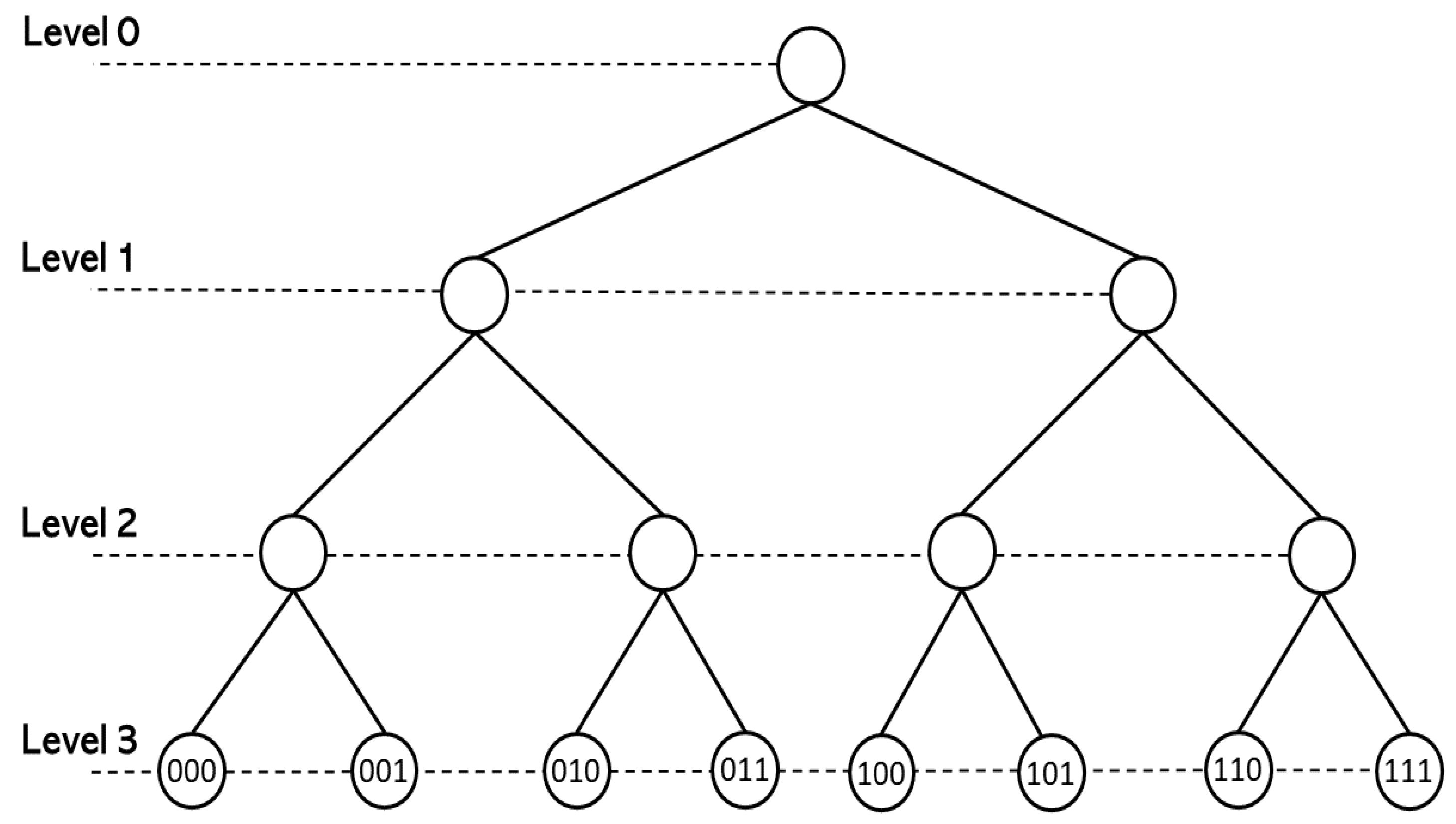
becomes a finite ultrametric space. In addition,
can be identified with the set of branches (vertices at the top level) of a rooted tree with
levels and
branches. By definition, the tree’s root is the only vertex at level 0. There are exactly
p vertices at level 1, which correspond with the possible values of the digit
in the
p-adic expansion of
i. Each of these vertices is connected to the root by a non-directed edge. At level
k, with
, there are exactly
vertices, and each vertex corresponds to a truncated expansion of
i of the form
. The vertex corresponding to
is connected to a vertex
at level
if and only if
is divisible by
. See
Figure 1. Balls
are infinite rooted trees.
4.2. The Haar Measure
Since
is a compact topological group, there exists a Haar measure
, which is invariant under translations, i.e.,
[
36]. If we normalize this measure by the condition
, then
is unique. It follows immediately that
In a few occasions, we use the two-dimensional Haar measure
of the additive group
to normalize this measure by the condition
. For a quick review of the integration in the
p-adic framework, the reader may consult [
33] and the references therein.
4.3. The Bruhat–Schwartz Space in the Unit Ball
A real-valued function
defined on
is
called Bruhat–Schwartz function (or a test function) if, for any
, there exists an integer
such that
The
-vector space of Bruhat–Schwartz functions supported in the unit ball is denoted by
. For
, the largest number
satisfying (
16) is called
the exponent of local constancy (or the parameter of constancy) of . A function
in
can be written as
where
,
, are points in
;
,
, are non-negative integers; and
denotes the characteristic function of ball
.
We denote by
the
-vector space of all test functions of the form
where
,
. Notice that
is supported on
and that
.
The space
is a finite-dimensional vector space spanned by the basis
By identifying
with the column vector
, we get that
is isomorphic to
endowed with the norm
Furthermore,
where ↪ denotes continuous embedding.
4.4. The p-Adic Version and Discrete Version of the Wilson–Cowan
Models
The
p-adic Wilson–Cowan model is obtained by taking
and
in (
10).
On the other hand,
, and
where
denotes the
-space of continuous functions on
endowed with the norm
. Furthermore,
is dense in
[
30] (Proposition 4.3.3); consequently, it is also dense in
and
.
For the sake of simplicity, we assume that
,
,
,
, and
,
. Theorem 1 is still valid under these hypotheses. We use the theory of approximation of evolution equations to construct good discretizations of the
p-adic Wilson–Cowan system; see, e.g., [
5] (Section 5.4).
This theory requires the following hypotheses.
(A) (a) and , , endowed with the norm are Banach spaces. It is relevant to mention that is a subspace of and that is a subspace of .
(b) The operator
is linear and bounded, i.e.,
and
, for every
.
(c) We set to be the identity operator. Then, , and , for every .
(d) , for , .
(
B,
C) The Wilson–Cowan system, see (
10), involves the operator
, where
is the identity operator. As approximation, we use
, for every
. Furthermore,
(see [
37] (Lemma 1)).
(
D) For
,
is continuous and such that, for some
,
for
,
f,
. This assertion is a consequence of the fact that
is well-defined, globally Lipschitz; see Lemma 1.
We use the notation
,
and, for the approximations,
,
. The space discretization of
p-adic Wilson–Cowan system (
10) is
The next step is to obtain an explicit expression for the space discretization given in (
17). We need the following formulae.
Remark 3. Let us takeThen,Indeed,By changing variables as , , in the integral,Now, by taking and using the fact that is an additive group, Remark 4. Let us take . Then,This formula follows from the fact that the supports of the functions , , are disjoint. The space discretization of the integro-differential equation in (
17) is obtained by computing the term
using Remarks 3 and 4. By using the notation
and for
,
,
With this notation, the announced discretization takes the following form:
Theorem 2. Let us take , , and . Let be solutions (11) and (12) given in Theorem 1. Let be the solution of Cauchy problem (17). Then, Proof. We first notice that Theorem 1 is valid for Cauchy problem (
17); more precisely, this problem has a unique solution
in
satisfying properties akin to the ones stated in Theorem 1. Since
is a subspace of
, by applying Theorem 1 to Cauchy problem (
17), we obtain the existence of a unique solution
in
satisfying the properties announced in Theorem 1. To show that the solution
belongs to
, we use [
5] (Theorem 5.2.2). For similar reasoning, the reader may consult Remark 2 and the proof of Theorem 1 in [
27]. The proof of the theorem follows from hypotheses A, B, C, and D according to [
5] (Theorem 5.4.7). For similar reasoning, the reader may consult the proof of Theorem 4 in [
27]. □
6. -Adic Kernels and Connection Matrices
There have been significant theoretical and experimental developments in comprehending the wiring diagrams (connection matrices) of the cerebral cortex of invertebrates and mammals over the last thirty years; see, for example, [
6,
7,
8,
9,
10,
11,
12,
13,
14,
15,
16,
17,
18,
19] and the references therein. The topology of cortical neural networks is described by connection matrices. Building dynamic models from experimental data recorded in connection matrices is a very relevant problem.
We argue that our
p-adic Wilson–Cowan model provides meaningful dynamics on networks whose topology comes from a connection matrix.
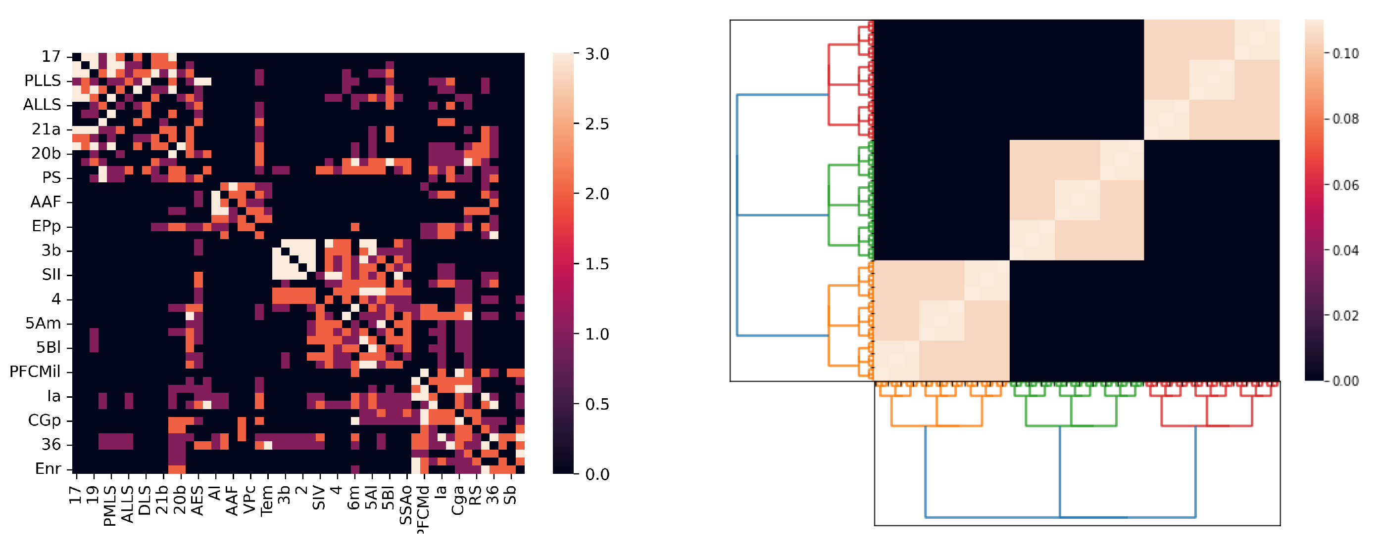
Figure 8 depicts the connection matrix of the cat cortex (see, e.g., [
7,
8,
9,
10,
11,
12,
13,
14]) and the matrix of the kernel
used in Simulation 1. The
p-adic methods are relevant only if the connection matrices can be very well approximated for matrices coming from discretizations of
p-adic kernels. This is an open problem. Here, we show that such an approximation is feasible for the cat cortex connection matrix.
Given an arbitrary matrix
A, by adding zero entries, we may assume that its size is
, where
p is a suitable prime number. We assume that
, where
is the ring of integers modulo
endowed with the
p-adic topology, as in the above. This hypothesis means that the connection matrices have an ultrametric nature; this type of matrices appear in connection with complex systems, such as spin glasses; see [
23] (
Section 4.2) and the references therein. Given an integer
r satisfying
, the reduction mod
map is defined as
. We now define
Map
induces a block decomposition of matrix
A into
blocks of size
. Given
, the corresponding block is
. Now, we attach to
,
and identify
with matrix
. By using the correspondence
we approximate matrix
A with a kernel
, which is locally translation invariant. More precisely, for each
,
for all
and
. Notice that if
, the matrix attached to
is
A. See
Figure 9. This procedure allows us to incorporate experimental data from connecting matrices into our
p-adic Wilson–Cowan model.
By using the above procedure, we replace the excitatory–excitatory relation term
with
but keep the other kernels as in Simulation 1. For the stimuli, we use
, with
,
, and
. In
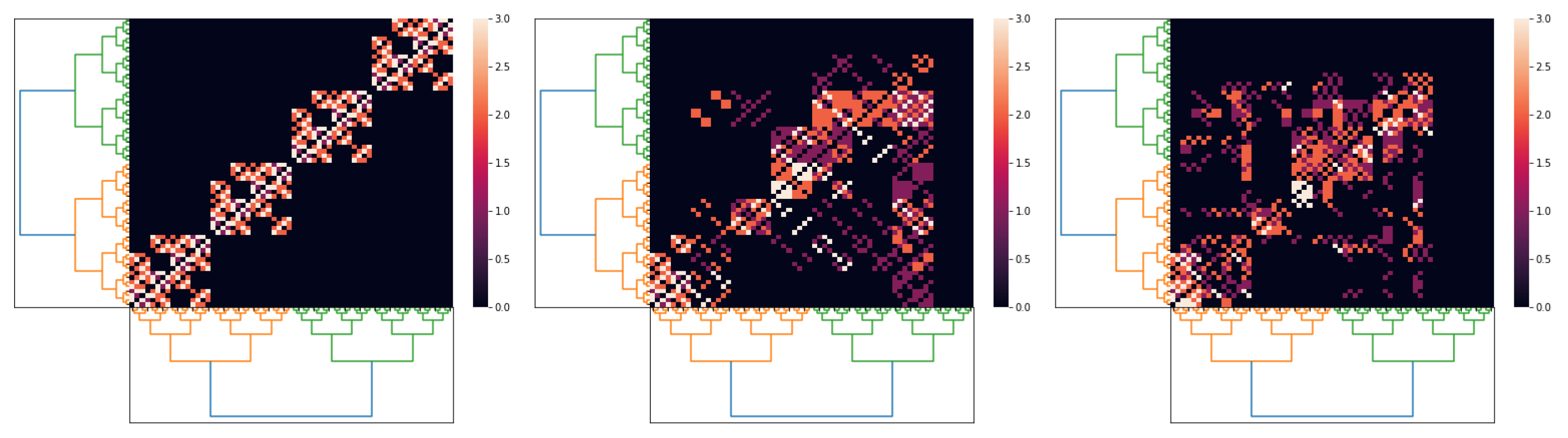
Figure 9, we show three different approximations for the cat cortex connection matrix using
p-adic kernels. The black area in the right matrix in
Figure 9 (which corresponds to zero entries) comes from the process of adjusting the size of the origin matrix to
.
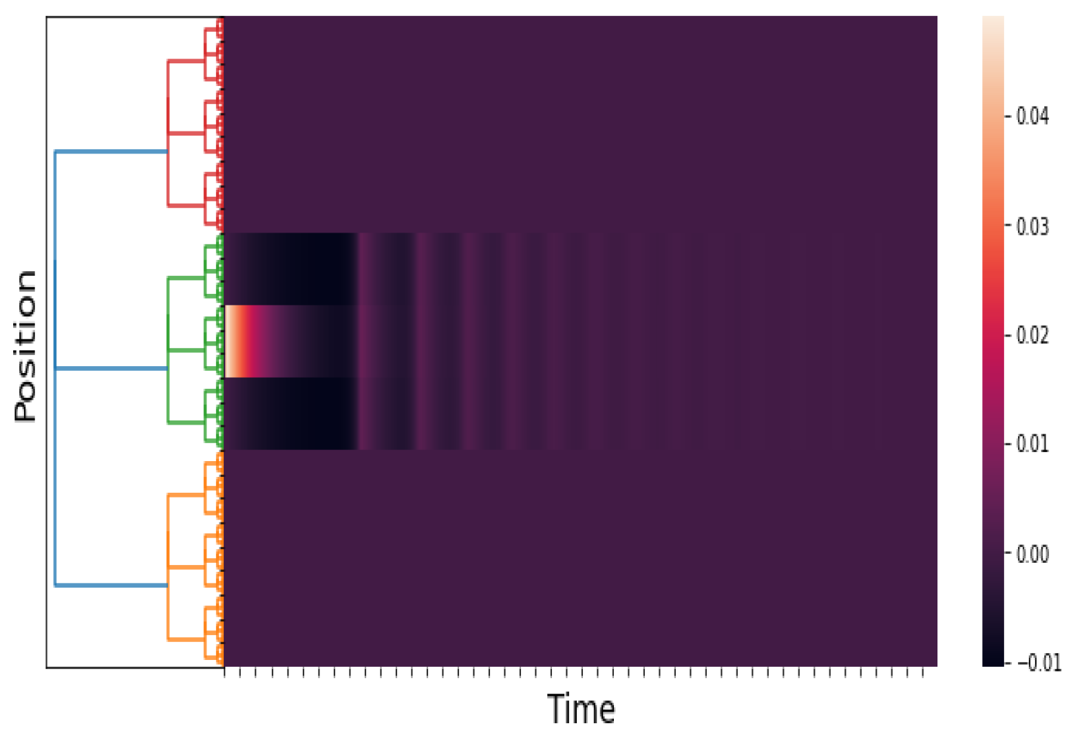
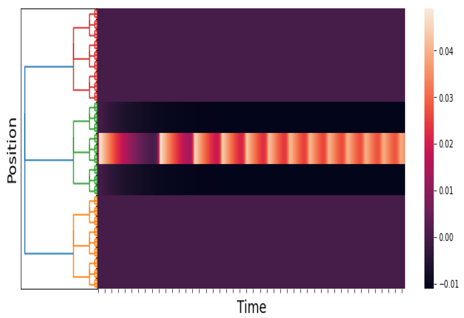
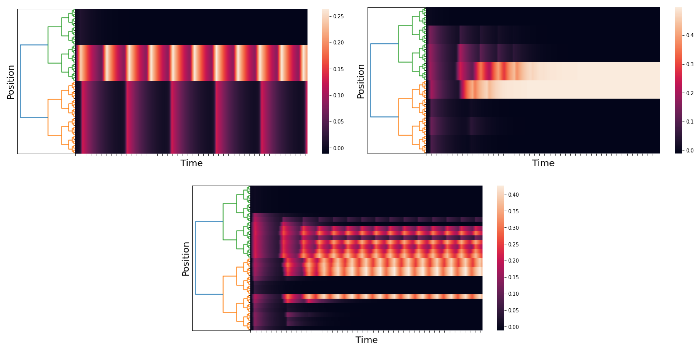
The corresponding
p-adic network responses are shown in
Figure 10 for different values of
r. In the case
, the interaction among neurons is short range, while in the case
, there is long-range interaction. The response in the case
is similar to the one presented in Simulation 1; see
Figure 5. When the connection matrix gets close to the cat cortex matrix (see
Figure 9), which is when the matrix allows more long-range connections, the response of the network presents more complex patterns (see
Figure 10).
7. Final Discussion
The Wilson–Cowan model describes interactions between populations of excitatory and inhibitory neurons. This model constitutes a relevant mathematical tool for understanding cortical tissue functionality. On the other hand, in the last twenty-five years, there has been tremendous experimental development in understanding the cerebral cortex’s neuronal wiring in invertebrates and mammalians. Employing different experimental techniques, the wiring patterns can be described by connection matrices. Such a matrix is just an adjacency matrix of a directed graph whose nodes represent neurons, groups of neurons, or portions of the cerebral cortex. The oriented edges represent the strength of the connections between two groups of neurons. This work explores the interplay between the classical Wilson–Cowan model and connection matrices.
Nowadays, it is widely accepted that the networks in the cerebral cortex of mammalians have the small-world property, which means a non-negligible interaction exists between any two groups of neurons in the network. The classical Wilson–Cowan model is not compatible with the small-world property. We show that the original Wilson–Cowan model can be formulated on any topological group, and the Cauchy problem for the underlying equations of the model is well posed. We give an argument showing that the small-world property requires that the group be compact, and consequently, the classical model should be discarded. In practical terms, the classical Wilson–Cowan model cannot incorporate the experimental information contained in connection matrices. We propose a p-adic Wilson–Cowan model, where the neurons are organized in an infinite rooted tree. We present numerical experiments showing that this model can explain several phenomena, similarly to the classical model. The new model can incorporate experimental information coming from connection matrices.


