
Fidelity Mechanics: Analogues of the Four Thermodynamic Laws and Landauer’s Principle

Abstract
:1. Introduction
- (i)
- There is long-standing folklore pointing towards a similarity between critical points and black holes, which usually refers to the fact that the effects from a critical point at zero temperature may be observed in a critical regime at low but finite temperature [51]. Given that both critical points and black holes originate from singularities, there should be a method for clarifying a formal similarity between QPTs and black holes.
- (ii)
- RG flows from an unstable fixed point to a stable fixed point are irreversible. This is relevant to Zamolodchikov’s c-theorem [52,53,54] and Cardy’s a-theorem [55,56], which may be regarded as the adaptation of the renowned Boltzmann’s H theorem to the RG setting. In real space RG theories, such as Kadanoff block spins as well as other coarse-graining RG schemes, high-energy degrees of freedom are discarded. Therefore, RG flows seem irreversible in a similar sense to the situations described by Boltzmann’s H theorem, where physical time is replaced by an RG parameter [57]. Thus, it is desirable to see if there are any intrinsic explanations for the irreversibility from the perspective of fidelity.
- (iii)
- As Landauer first noted [58], at finite temperature T, in order to erase one bit of information, we need to perform minimum work w: , with being the Boltzmann constant. At zero temperature, do we still need to perform any minimum work to erase one bit of information?
- (iv)
- During the construction of an effective Hamiltonian along any RG flow, an unlimited number of irrelevant coupling constants proliferate. In practice, this prevents access to a stable fixed point. It is tempting to see if there is any deep reason underlying this observation.
- (v)
- A proper definition of QPTs is still lacking. Traditionally, the ground-state energy density is used as an indicator to signal a critical point, but it fails in many situations [59]. Instead, some exotic indicators, such as entanglement entropy [60], topological entanglement entropy [61,62], and the ground-state fidelity per lattice site [26,27,28], are introduced to signal QPTs due to recent progress in our understanding of quantum critical phenomena. Therefore, it is important to find a proper criterion to define QPTs.
2. Fidelity Mechanics: Basic State Functions
2.1. Preliminaries
2.1.1. Quantum Many-Body Systems: Six Illustrative Models
2.1.2. Ground-State Fidelity per Lattice Site
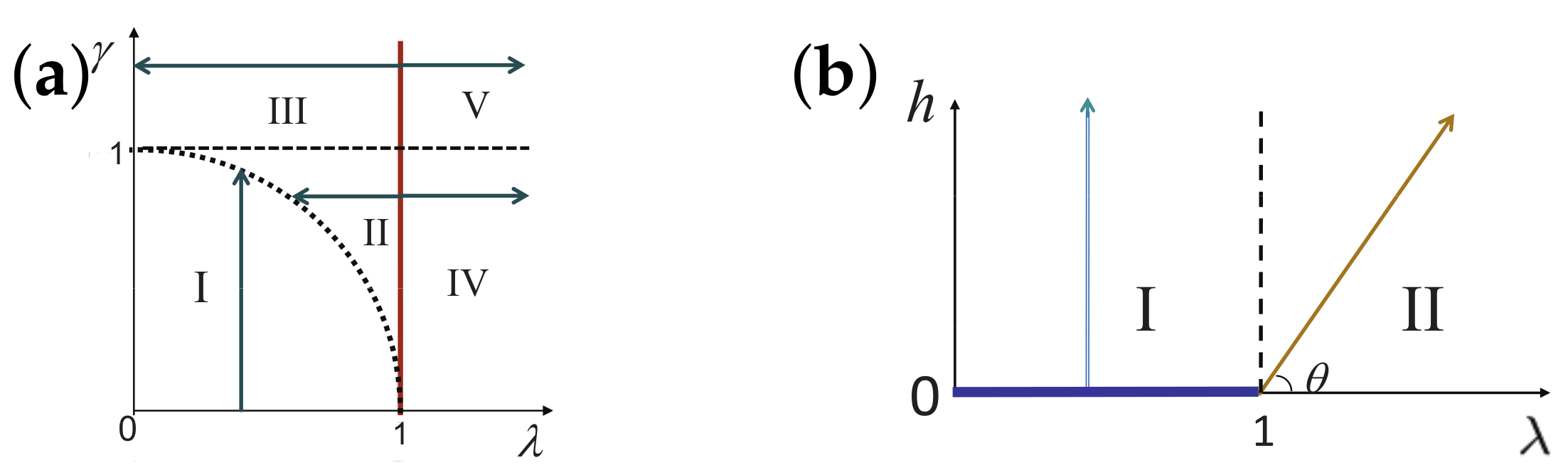
2.1.3. A Characteristic Line and a Characteristic Point
- (i)
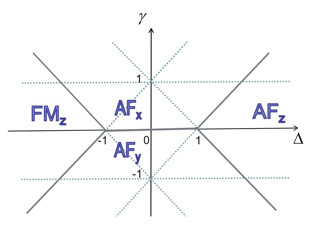
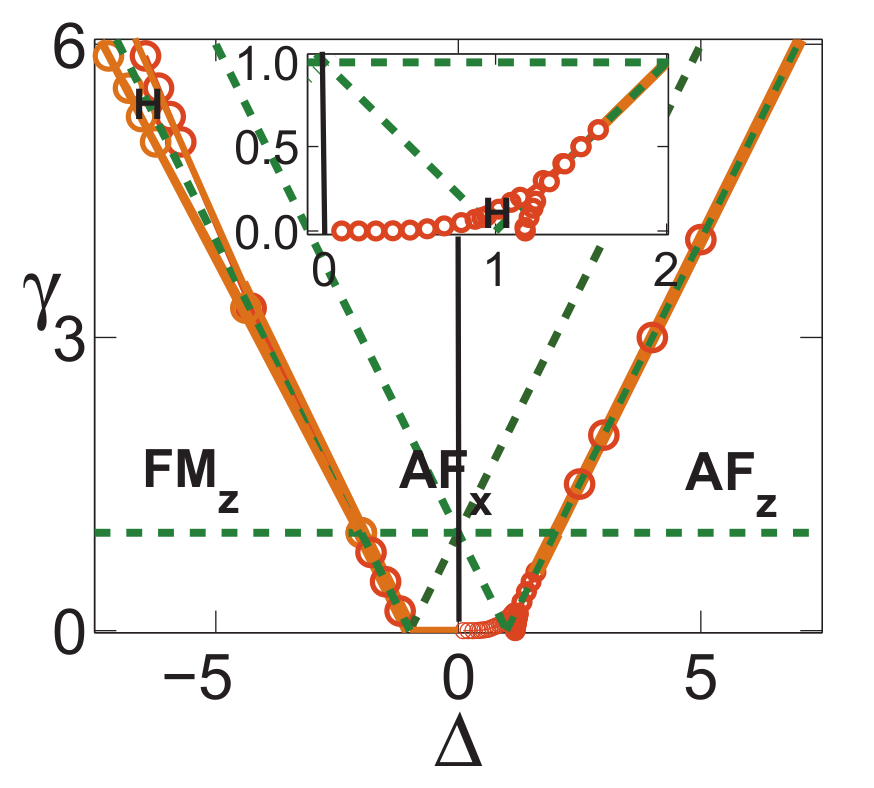
- Generically, the symmetry group of the Hamiltonian varies with coupling parameters and . If the Hamiltonian possesses a distinct symmetry group when the coupling constants take special values on a characteristic line in a given phase, then it separates this phase into different regimes in the control parameter space. An example to illustrate this observation is the quantum spin- XYZ model (3). For this model, on the line (), the Hamiltonian possesses symmetry, which is lost when coupling parameters move away from this characteristic line. In particular, a symmetry occurs when one coupling parameter is infinite in value. This type of characteristic line is referred to as a symmetric line.
- (ii)
- Characteristic lines also arise from dualities [3,76], which are defined via a local or nonlocal unitary transformation, and they separate a given phase into different regimes in the control parameter space. An example to illustrate this observation is the quantum spin- XY model (1) [3,76]. Dualities exist along the two lines ( and ). This type of characteristic line is referred to as a dual line. Caveat: Sometimes it is a bit tricky to recognize a dual line as a type of characteristic line. Suppose dualities exist on a plane. Then, the plane itself is a characteristic plane. Generically, a line in this plane is not a characteristic line, unless this line is self-dual in nature. However, if a line turns out to be a dual line for a sub-model, with one of the two control parameters being zero, then it is also recognized as a characteristic line for the full model. Mathematically, this amounts to stating that such a characteristic line is semi-self-dual in the sense that only one of the two coupling parameters remains to be the same. This is seen in the quantum spin- XYZ model (3) and the quantum spin-1 XYZ model (5).
- (iii)
- Another type of characteristic line comes from factorizing fields [77,78,79,80,81,82]. Indeed, apart from various analytical approaches, there is an efficient numerical means for identifying factorizing fields for quantum many-body systems in the context of tensor networks [70,71] (also cf. Appendix B). A line of factorizing fields divides a specific phase into different regimes. Examples to illustrate this observation are the quantum spin- XY model (1) and the quantum spin- XYZ model (3) [77,78,79,80,81,82]. An interesting feature for a line of factorizing fields is that they frequently occur in a symmetry-broken phase and, in turn, are frequently associated with the PT transitions and FM transitions. We remark that factorizing fields also occur when one coupling parameter takes infinity in value or when more than one coupling parameters are infinite in value. This type of characteristic line is referred to as a factorizing-field line.
- (iv)
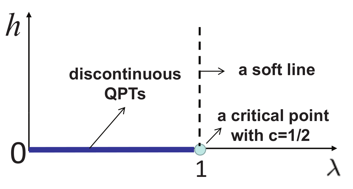
- There is a peculiar type of characteristic line, originating from an isolated critical or a multi-critical point and ending at a point on a symmetric line, a dual line, or a factorizing-field line. This type of characteristic line is needed, if any other type of characteristic line is absent at such an isolated critical point or a multi-critical point. An illustrative example is a characteristic line () for the transverse-field quantum Ising model in a longitudinal field (2). This type of characteristic line is referred to as a soft line due to the fact that this type of characteristic line does not impose any rigid constraints in a sense that its location in the control parameter space is not fixed in contrast to the constraints imposed by a symmetric line, a dual line, and a factorizing-field line.
2.1.4. A Principal Regime
2.1.5. A Dominant Control Parameter x and an Auxiliary Control Parameter
2.1.6. Nineteen Principal Regimes for the Six Illustrative Models
2.2. A Fidelity Mechanical System and Its Environment
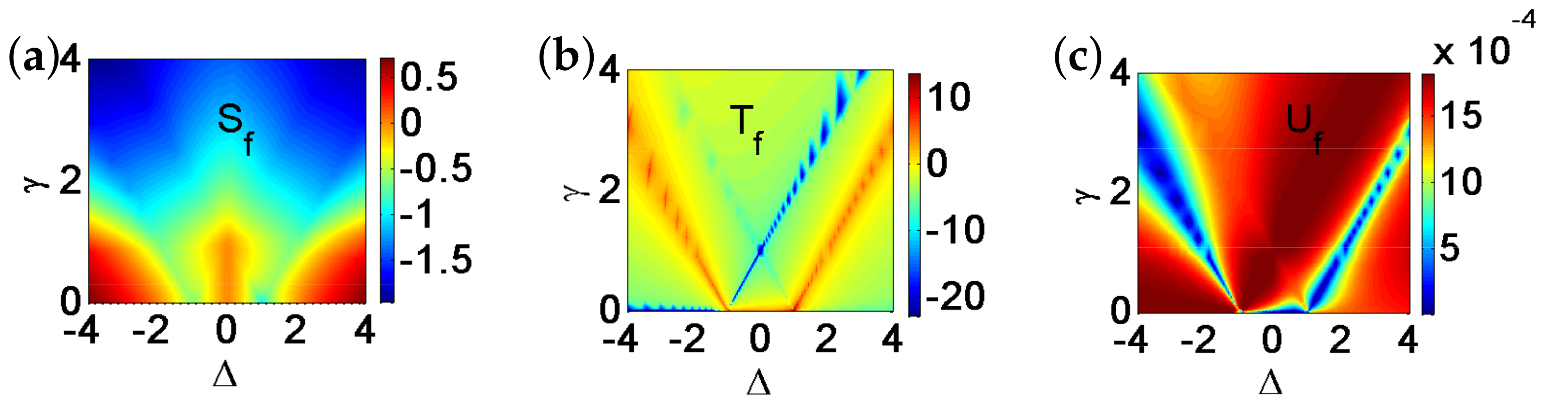
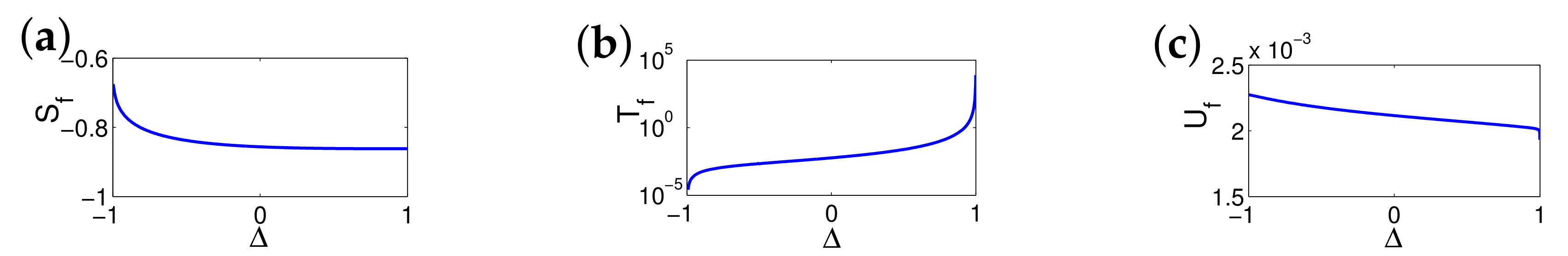
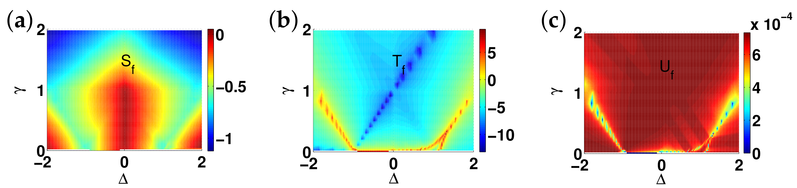
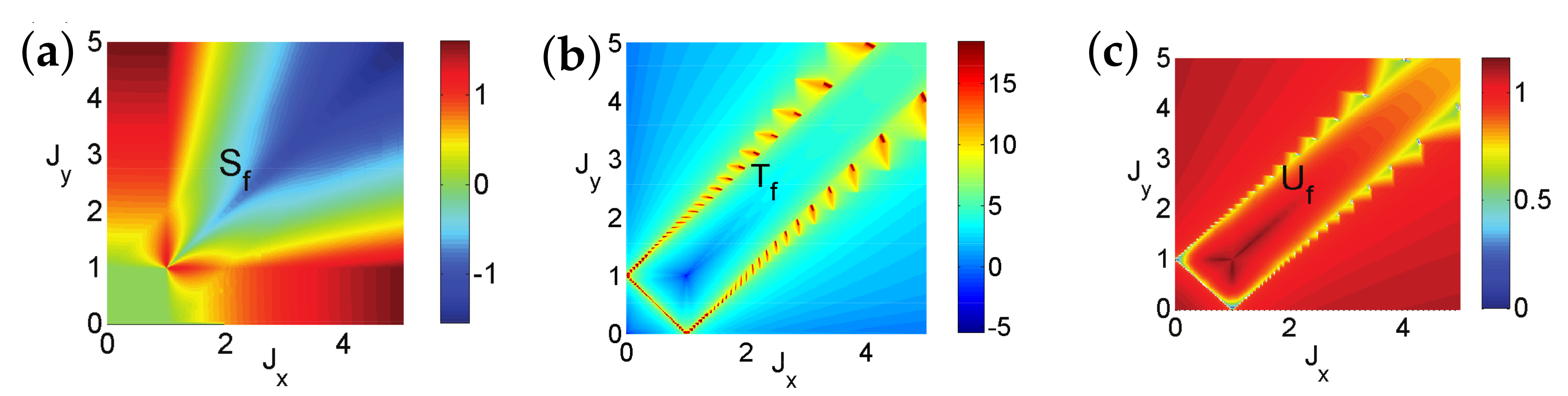
2.3. Fidelity Entropy, Fidelity Temperature, and Fidelity Internal Energy: Continuous Quantum Phase Transitions
2.4. Fidelity Entropy, Fidelity Temperature, and Fidelity Internal Energy: Discontinuous Quantum Phase Transitions
2.5. Relation between an Unknown Function and Fidelity Temperature
- (A)
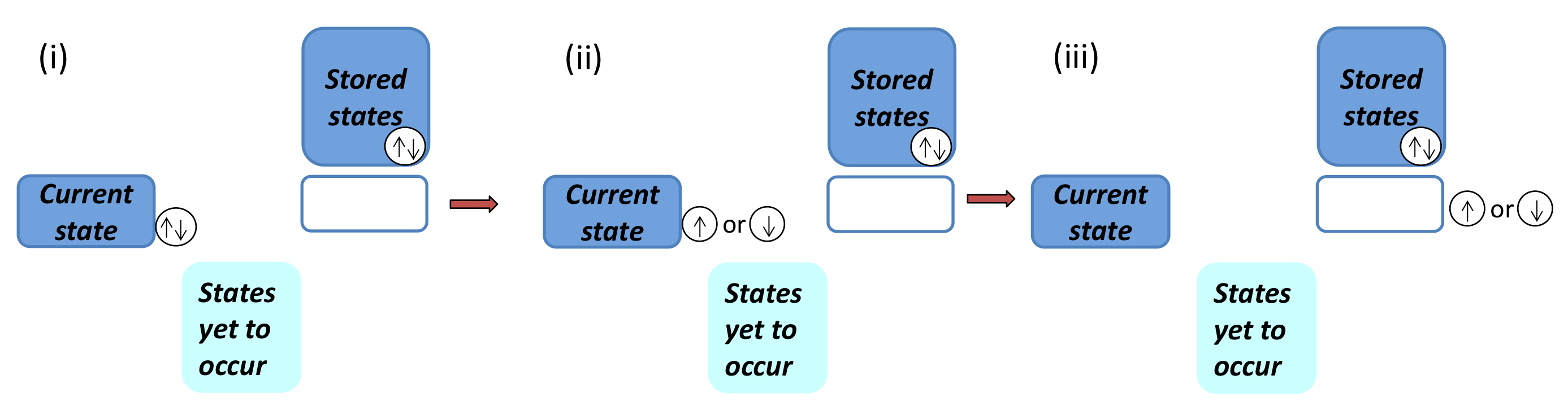
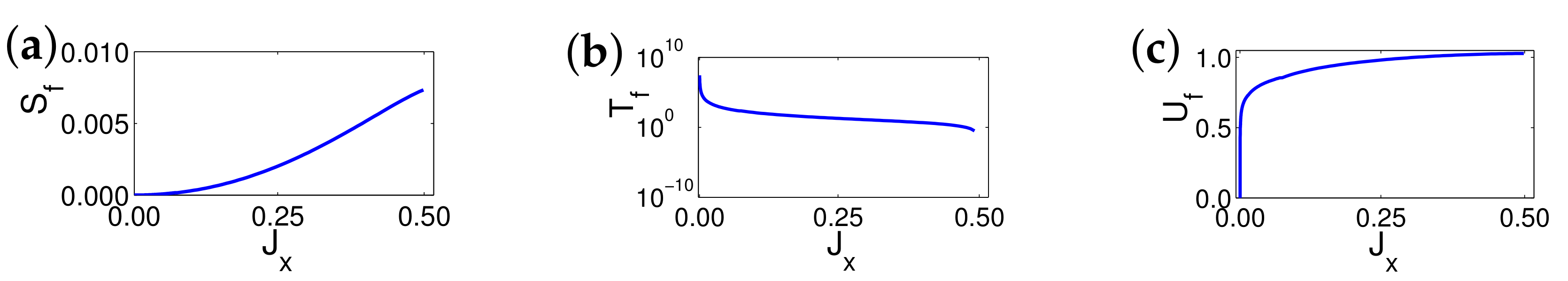
- For a single-copy system, if the ground-state energy density monotonically decreases from a critical point to x, then fidelity internal energy takes the following form: , with being an additive constant, and being positive. For a composite system consisting of two identical copies, fidelity mechanical-state functions remain the same as a single-copy system. This is illustrated in Figure 5i. Now, one copy is deleted from a composite fidelity mechanical system for a value of a dominant control parameter between x and . To perform the deletion, a certain amount of fidelity work, quantifying the computational costs, , needs to be performed, as required by the analogue of Landauer’s principle at zero temperature, to compensate for the increment of fidelity internal energy , as illustrated in Figure 5iiAs the last step, which is illustrated in Figure 5iii, the information about the retained copy is removed from the current state media and recorded in the information storage media. This amounts to extracting one bit of information for each value of a dominant control parameter between x and , thus leading to a change in fidelity entropy:That is, is required to be related with as followsIf , then we have the following
- (B)
- For a single-copy system, if the ground-state energy density monotonically increases from a critical point to x, then fidelity internal energy takes the following form: , with being an additive constant, and being positive. For a composite system consisting of two identical copies, fidelity mechanical-state functions remain the same as a single-copy system. This is illustrated in Figure 5i. Now, one copy is deleted from a composite fidelity mechanical system for a value of a dominant control parameter between x and . To perform this deletion, a certain amount of fidelity work, quantifying the computational costs, needs to be performed, as required by the analogue of Landauer’s principle at zero temperature, to compensate for the increment of fidelity internal energy , as illustrated in Figure 5ii:As the last step, which is illustrated in Figure 5iii, the information about the retained copy is removed from the current state media and recorded in the information storage media. This amounts to extracting one bit of information for each value of a dominant control parameter between x and , thus leading to a change in fidelity entropy—:That is, is required to be related with as followsIf , then we have the following

2.6. A Contribution to Fidelity Entropy from Rescaling in the Ground-State Energy Density
2.7. Shifts in Fidelity Temperature and Fidelity Internal Energy
2.8. Piecing Together All Regimes: The Continuity Requirements
2.8.1. The Continuity Requirements for Fidelity Entropy: A Characteristic Point, a Characteristic Line, and a Principal Regime
2.8.2. The Continuity Requirements for Fidelity Temperature and Fidelity Internal Energy: A Characteristic Line
2.8.3. The Continuity Requirements for Fidelity Temperature and Fidelity Internal Energy: A Principal Regime
2.8.4. The Continuity Requirements for Fidelity Temperature and Fidelity Internal Energy: Discontinuous Phase Transitions
2.8.5. Piecing Together Principal Regimes and Non-Principal Regimes (If Any)
2.9. Generic Remarks
3. A Shift Operation in the Hamiltonian: Duality and a Canonical Form of the Hamiltonian
4. A Fictitious Parameter Connecting Different Choices for a Dominant Control Parameter in a Principal Regime
5. Fidelity Mechanical-State Functions under a Shift Operation in the Hamiltonian with Respect to a Reference Benchmark
6. A Characterization of Quantum Phase Transitions and Quantum States of Matter in Fidelity Mechanics
6.1. An Interior Point of View vs. an Exterior Point of View
6.2. A Characterization of Quantum Phase Transitions in Fidelity Mechanics
6.3. A Characterization of Topological Quantum States of Matter in Fidelity Mechanics
7. Quantum Spin- XY Model—A Typical Example for Continuous Quantum Phase Transitions
8. Transverse-Field Quantum Ising Model in a Longitudinal Field—A Typical Example for Discontinuous Quantum Phase Transitions
9. Quantum Spin- XYZ Model—A Typical Example for Dualities
10. Quantum Spin- XXZ Model in a Magnetic Field—An Intermediate Case between the Kosterlitz–Thouless Transitions and the Pokrovsky–Talapov Transitions
11. Quantum Spin-1 XYZ Model—A Typical Example for the Symmetry-Protected Topological Phases
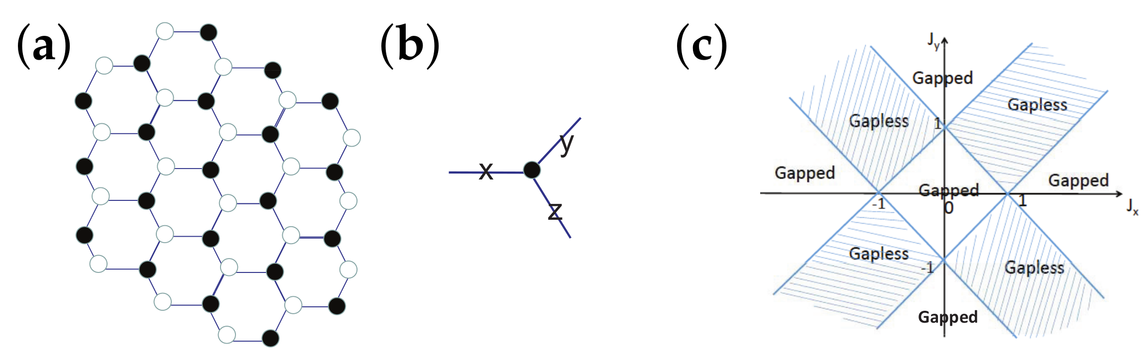
12. The Spin- Kitaev Model on a Honeycomb Lattice—A Typical Example for Topologically Ordered States
13. Analogues of the Four Thermodynamic Laws, Fidelity Flows and Miscellanea
13.1. Analogues of the Four Thermodynamic Laws
- (i)
- Zeroth law—for a given fidelity mechanical system, which is in equilibrium with its environment, fidelity temperature quantifies quantum fluctuations.
- (ii)
- First law—fidelity internal energy may be transferred from a fidelity mechanical system, as fidelity work or fidelity heat (defined via fidelity entropy), to its environment or vice versa. Mathematically, we have .
- (iii)
- Second law—the total fidelity entropy of a fidelity mechanical system and its environment never decreases. Physically, this amounts to stating that the information gain we are able to recover from the environment never exceeds information loss incurred due to information erasure in a fidelity mechanical system. Mathematically, we have. Generically, and . Therefore, , with being defined by .
- (iv)
- Third law—for a fidelity mechanical system, fidelity entropy approaches a (local) maximum and fidelity temperature approaches zero, as a stable fixed point is approached. However, the probability for accessing a stable fixed point is zero.
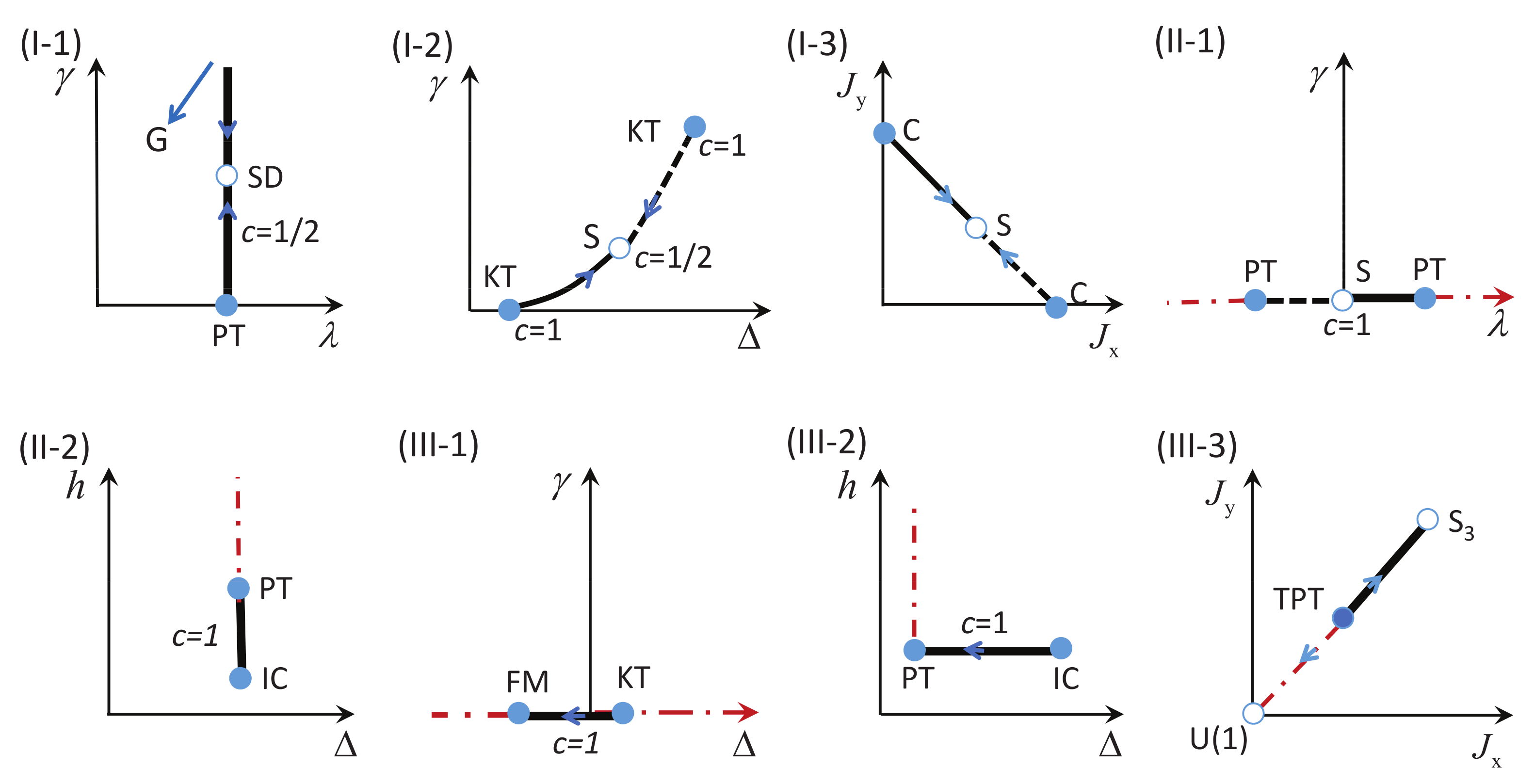
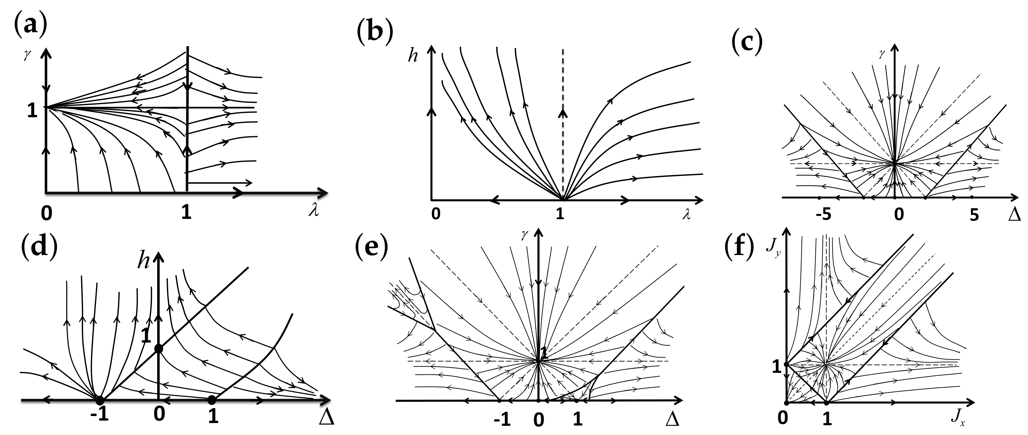
13.2. Fidelity Flows as an Alternative Form of RG Flows
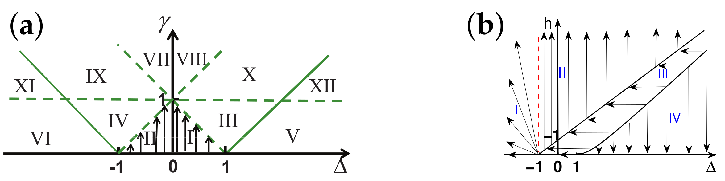
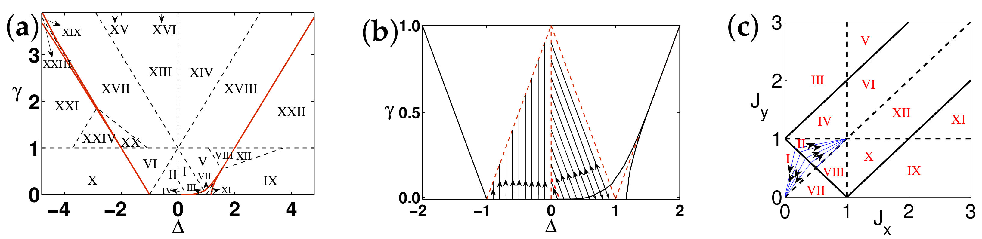
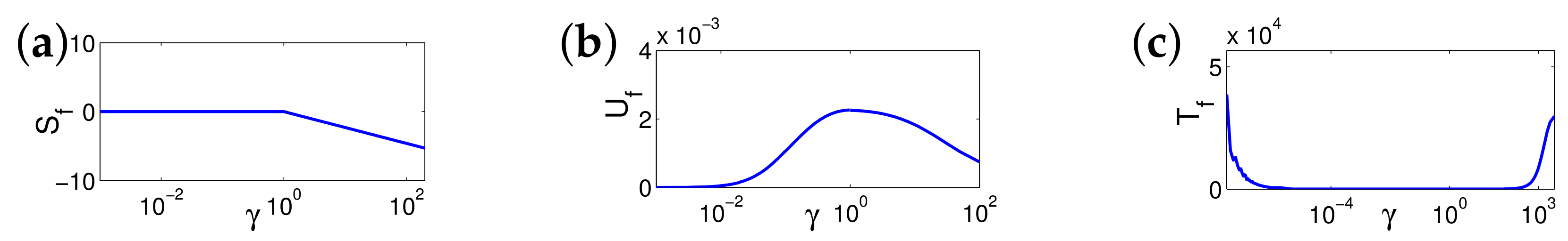
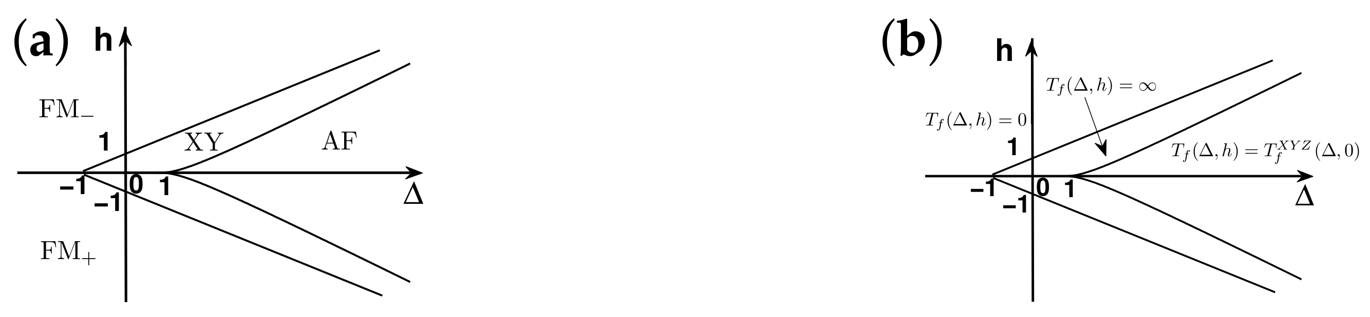
- (a)
- For the quantum spin- XY model ( and ), two stable fixed points are identified for the Ising universality class at (0, 1) and (∞, 1), which is protected by the symmetry, and one stable fixed point for the PT universality class at (∞, 0), which is protected by the symmetry. For the Ising universality class, a symmetry emerges at (0, 1) and (∞, 1), in addition to the symmetry, whereas for the PT universality class, a symmetry, defined by , , and , , , emerges at (∞, 0), in addition to the symmetry. Generically, it is the emergence of such an extra symmetry at a stable fixed point that justifies why it is not accessible. On the other hand, given two lines of critical points belonging to two different universality classes, we interpret the disordered circle as a separation line between two different types of fidelity flows, with one type of fidelity flows starting from unstable fixed points with central charge , and the other type of fidelity flows starting from unstable fixed points with central charge . Note that both types of fidelity flows end at the same stable fixed point , at which fidelity entropy reaches a local maximum. From an interior point of view, no fidelity flow exists on the line of the Gaussian critical points ( with ), reflecting the fact that this line of critical points originates from the level crossings; thus, the ground-state fidelity per lattice site is zero. On the Ising line of critical points ( with ), central charge c is 1 when is infinite in value, and c is , when is finite and non-zero. Therefore, fidelity flows start from (1, ∞) to (1, 1) and from (1, 0) to (1, 1).
- (b)
- For the transverse-field quantum Ising model in a longitudinal field (), two stable fixed points (0, 0) and (∞, 0) are identified for the Ising universality class, which is protected by the symmetry, and one stable fixed point (1, ∞) is identified for the Ising universality class without any symmetry, corresponding to the Hamiltonian with and . In addition, there is one stable fixed point (0, ∞) protected by the symmetry when . Indeed, (1, ∞) should be identified with (0, ∞). Note that an extra symmetry emerges at stable fixed points (0, 0), (∞, 0), and (1, ∞), and an extra symmetry, defined by , , and , , , emerges at a stable fixed point (0, ∞). This justifies why a stable fixed point is not accessible.
- (c)
- For the quantum spin- XYZ model (), three stable fixed points are identified for the Gaussian universality class at (0, 1) and (, 1), and two stable fixed points are identified for the KT universality class at (0, 1) and (∞, 0). In addition, a stable fixed point (−∞, 0) originates from the FM transition point at (, 0). Both the KT and FM transitions are protected by the symmetry as well as the dihedral symmetry group and the time-reversal symmetry group . The fact that (∞, 1) and (∞, 0) represent two different stable fixed points may be understood from both symmetry-breaking order and RG flows. In fact, a symmetry exists on the line ( with ), where is generated by : and , and is generated by the one-site translation : , with . However, only two-fold degeneracies exist, with each degenerate ground state invariant under the combined action , which generates another . Thus, the symmetry group, which is spontaneously broken, is . This is different from the cases with non-zero , in which the spontaneously broken symmetry group is . This also matches an observation that, for , there is a symmetry, which protects the KT transition. Once becomes nonzero, the symmetry is lost, and a continuous QPT changes from the KT universality class to the Gaussian universality class. In addition, it is the emergence of an extra symmetry at a stable fixed point, such as a symmetry at (0, 1) and (, 1), and a symmetry, defined by , , and , , , at (∞, 0) that justifies why a stable fixed point is not accessible. From an interior point of view, fidelity flows exist on the line of the Gaussian critical points ( with ), starting from (1, 0), and ending at (, 0); on the line of the Gaussian critical points ( with ), starting from () and ending at (1, 0); on the line of the Gaussian critical points ( with ), starting from (, 0) and ending at ().
- (d)
- For the quantum spin- XXZ model in a magnetic field, two stable fixed points (0, ∞) and (, 0) are identified for the PT universality class; one stable fixed point (−∞, 0) originates from the FM transition point and one stable fixed point (∞, 0) is identified for the KT universality class, protected by the symmetry, as well as the dihedral symmetry group and the time-reversal symmetry group . From an interior point of view, fidelity flows exist in the XY critical regime, starting from an IC transition point on the phase boundary between the XY phase and the AF phase and ending at the line of the PT transition points ( with ), in contrast to the chosen dominant control parameter x, which is in parallel to the horizontal axis, with h fixed. This is because any two ground states with different values of h for a given in the XY critical regime are orthogonal to each other due to the level crossings.
- (e)
- For the quantum spin-1 XYZ model (), three stable fixed points (0, 1) and (, 1) are identified for the Gaussian universality class; one metastable fixed point (1, 0) is identified for the KT universality class, one stable fixed point (, 0) is identified for the FM transition point , both of which are protected by the symmetry, as well as the dihedral symmetry group and the time-reversal symmetry group , and two stable fixed points and (∞, 0) and one metastable fixed point are identified for the Ising universality class. Note that, for a stable or metastable fixed point, its symmetric or dual images also constitutes a stable or metastable fixed point. From an interior point of view, fidelity flows exist on the line of the Gaussian critical points: with , starting from (, 0) and ending at the FM transition point (, 0). Here, is the KT transition from the critical XY phase to the Haldane phase on the -symmetric line (). This also happens on the dual image lines. In addition, fidelity flows exist on the phase boundaries between the Haldane phase and the symmetry-breaking ordered AF phases.
- (f)
- For the spin- Kitaev model on a honeycomb lattice ( and ), in addition to three stable fixed points , , and , and are also identified as stable fixed points in the gapped phases due to the variation of the symmetry group, although and may be identified with and . One stable fixed point is identified in the gapless spin liquid phase. From an interior point of view, fidelity flows exist on the boundaries between the gapless spin liquid phase and the gapped spin liquid phase: with and its dual image lines. For with , fidelity flows start from the transition points and and end at the -symmetric point .

13.3. Miscellanea
14. Outlook
15. Conclusions
Author Contributions
Funding
Data Availability Statement
Acknowledgments
Conflicts of Interest
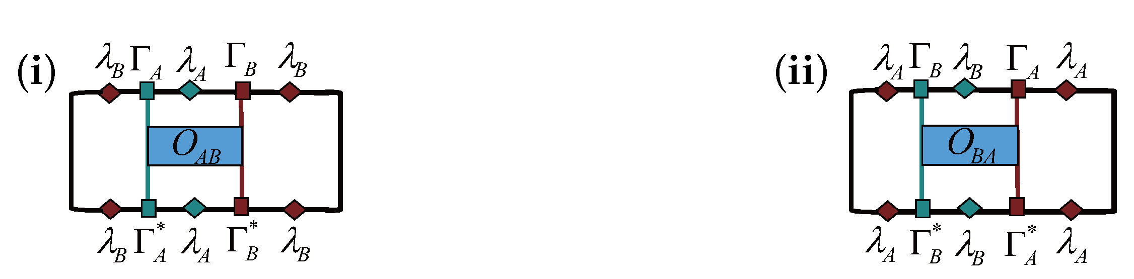
Appendix A. Relevant and Irrelevant Information via the Ground-State Fidelity per Lattice Site


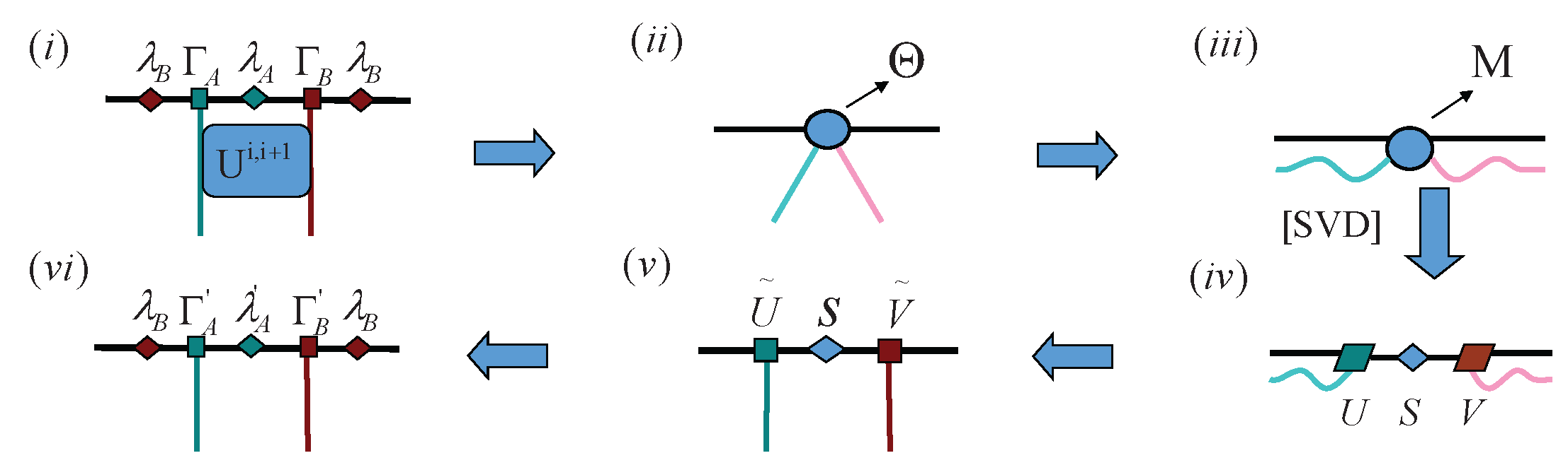
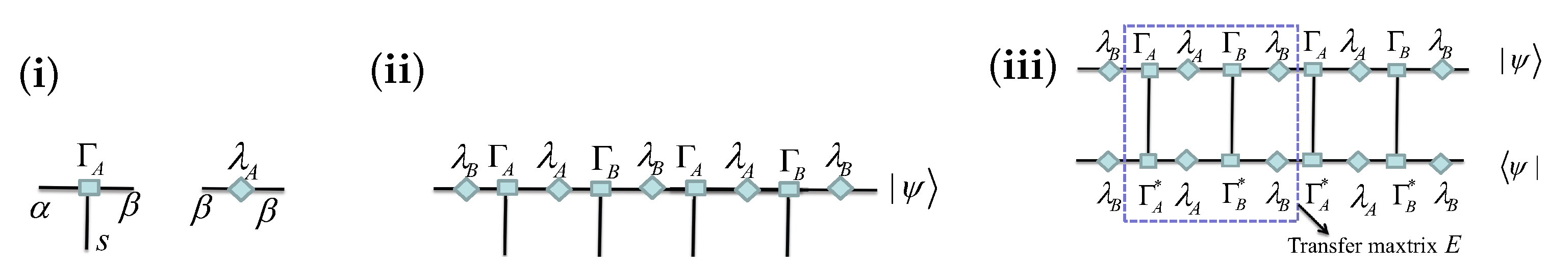
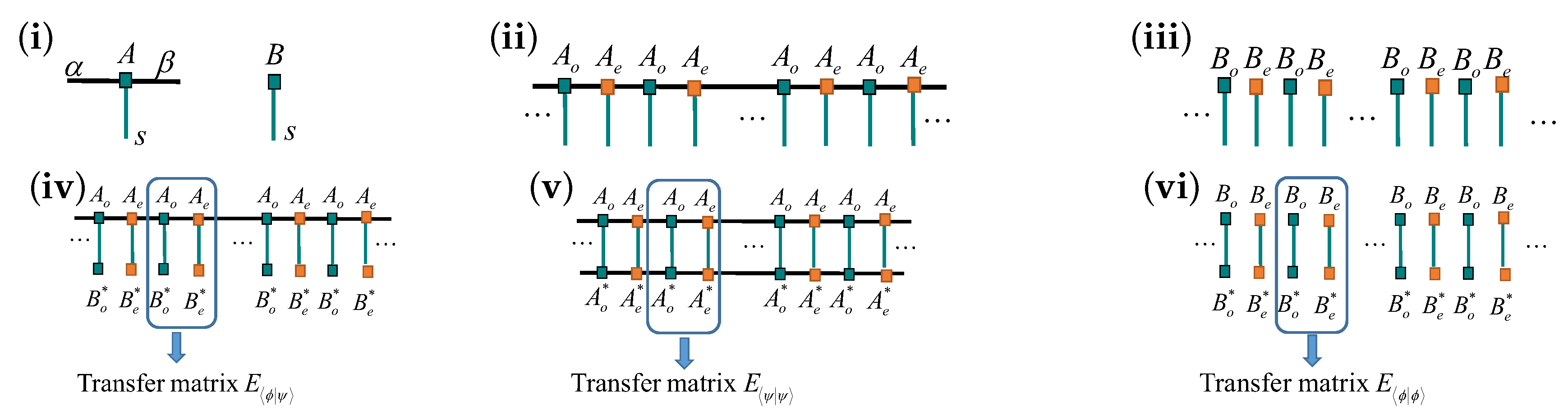
Appendix B. Ground-State Fidelity and Geometric Entanglement from Tensor Networks: Matrix-Product States
Appendix B.1. The Infinite Time-Evolving Block Decimation Algorithm


Appendix B.2. Ground-State Fidelity per Lattice Site

Appendix B.3. Geometric Entanglement

Appendix C. Dualities for the Quantum Spin- XYZ Model and the Spin- Kitaev Model on a Honeycomb Lattice
Appendix C.1. The Quantum Spin- XYZ Model
- (1)
- The Hamiltonian for is dual relative to the Hamiltonian for under a local unitary transformation : , , , , and : , with , , and . The Hamiltonian is self-dual when and .
- (2)
- Under a local unitary transformation : , , , we have , with ,, and . The Hamiltonian on the line () is self-dual.
- (3)
- Under a local unitary transformation : , , ,, and , we have, with , , and. The Hamiltonian on the line () is self-dual.
- (4)
- Under a local unitary transformation : , , , we have , with ,, and . The Hamiltonian on the line () is self-dual.
- (5)
- Under a local unitary transformation : , , ,, and , we have, with , , and. The Hamiltonian on the line () is self-dual.
Appendix C.2. The Spin- Kitaev Model on a Honeycomb Lattice
- (a)
- A local unitary transformation : , , , , and , accompanied by the lattice symmetry between the -bonds and the -bonds.
- (b)
- A local unitary transformation : , , , , , , , and , accompanied by the lattice symmetry between the -bonds and the -bonds.
- (1)
- The Hamiltonian is dual to the Hamiltonian under a local unitary transformation : , , , accompanied by the lattice symmetry between the -bonds and the -bonds, , with , , and . The Hamiltonian is self-dual when .
- (2)
- The Hamiltonian is dual to the Hamiltonian under a local transformation : , , , accompanied by the lattice symmetry between the -bonds and the -bonds, , with , , and . The Hamiltonian is self-dual when .
- (3)
- For , the Hamiltonian is dual to the Hamiltonian under a local transformation : , , , , and , accompanied by the lattice symmetry between the -bonds and the -bonds, , with , , and . The Hamiltonian is self-dual when .
- (4)
- For , the Hamiltonian is dual to the Hamiltonian under a local transformation : , , , , and , accompanied by the lattice symmetry between the -bonds and the -bonds, , with , , and . The Hamiltonian is self-dual when .
Appendix D. Thermodynamic Arrow of Time, Psychological/Computational Arrow of Time, and Cosmological Arrow of Time
Appendix E. Three Theorems in Quantum Information Science
- (a)
- No-cloning theorem: It is impossible to create an identical copy of an arbitrary unknown quantum state. The theorem was first articulated in Refs. [213,214]. It has profound implications in quantum information processing. Mathematically, the no-cloning theorem states that for an arbitrary normalized state on a system and an arbitrary normalized state on a system , there is no unitary operator satisfying , with depending on and .
- (b)
- No-deleting theorem: It appears as time-reversed and so is dual to the no-cloning theorem. Given two copies of some arbitrary quantum state, it is impossible to delete one of the copies [215]. Mathematically, suppose is an unknown quantum state in a Hilbert space. Then, there is no linear isometric transformation such that , with the final state of the ancilla being independent of .
- (c)
- No-hiding theorem: If information is missing from a given system due to interaction with the environment, then it is simply residing somewhere else. In other words, the missing information cannot be hidden in the correlations between a system and its environment. It was formalized in Ref. [216] and experimentally confirmed in Ref. [217].
Appendix F. Three Extensions
Appendix F.1. Fidelity Internal Energy , Fidelity Entropy , and Fidelity Temperature When the Ground-State Energy Density Is Always Positive
Appendix F.2. Fidelity Entropy, Fidelity Temperature, and Fidelity Internal Energy for Non-Translation-Invariant Quantum Many-Body Systems
Appendix F.3. Fidelity Entropy, Fidelity Temperature, and Fidelity Internal Energy at Finite Temperature
Appendix G. Scaling Entropy
Appendix G.1. The Quantum Spin- XYZ Model
Appendix G.2. The Quantum Spin-1 XYZ Model
Appendix G.3. The Spin- Kitaev Model on a Honeycomb Lattice
Appendix H. A Scaling Analysis of Fidelity Entropy in the Vicinity of a Critical/Transition Point and Beyond
Appendix H.1. A Scaling Analysis of Fidelity Entropy in the Vicinity of a Critical/Transition Point
Appendix H.2. A Scaling Analysis of the Ground-State Energy Density Close to a Gaussian Critical Point for the Quantum Spin- XY Model
Appendix I. A Universal Logarithmic Scaling of the Entanglement Entropy with a Block Size for Scale-Invariant States Arising from Spontaneous Symmetry-Breaking with Type-B Goldstone Modes

Appendix J. The Bond-Centered Nonlocal Order Parameter for the Symmetry-Protected Topological Phases and the Site-Centered Nonlocal Order Parameter for the Symmetry-Protected Trivial Phases

Appendix K. Fidelity Entropy , Fidelity Temperature , and Fidelity Internal Energy for the Quantum Spin- XY Model
- (i)
- If , then the Hamiltonian (1) is reduced to the transverse-field quantum Ising model . Hence, under the Kramers–Wannier unitary transformation : , and , we have , with and . The self-dual point is located at .
- (ii)
- If , then the Hamiltonian (1) is simplified to . Under a unitary transformation : , , , , , and , we have , with and . The self-dual point is located at .
Appendix K.1. Fidelity Entropy , Fidelity Temperature , and Fidelity Internal Energy : An Exterior Point of View
- (1)
- In part i ( with ), we recall that a dominant control parameter was chosen to be . From Equation (9), fidelity entropy takes the following form:Here, denotes the ground-state fidelity per lattice site in part i, and is the residual fidelity entropy at the critical point . According to our convention (cf. Section 2), we have .
- (2)
- (3)
- In part v, we recall that a dominant control parameter was chosen to be , starting from the PT transition point up to the -symmetric point on the disordered circle: . Given an exotic QPT that exists at the PT transition point on the disordered circle [59], we need to treat it separately. From Equation (9), fidelity entropy takes the same form as Equation (A43) for part i, with the label being changed from i to v. According to our convention (cf. Section 2), we have .
- (a)
- In regime ( and ), we recall that a dominant control parameter was chosen to be and an auxiliary control parameter was chosen to be . From Equation (28), fidelity entropy takes the following formHere, denotes the ground-state fidelity per lattice site in regime , and is the residual fidelity entropy at a critical point for a fixed , with . According to our convention (cf. Section 2), we have .
- (b)
- In regime ( and ), we recall that a dominant control parameter was chosen to be and an auxiliary control parameter was chosen to be . From Equation (28), fidelity entropy takes the same form as Equation (A44) for regime I, with the label being changed from I to II. According to our convention (cf. Section 2), we have .
- (c)
- In regime ( and ), we recall that a dominant control parameter was chosen to be and an auxiliary control parameter was chosen to be . From Equation (28), fidelity entropy takes the same form as Equation (A44) for regime I, with the label being changed from I to III. In this regime, the continuity requirement for on the dual line, labelled as iv, implies that includes a contribution from scaling entropy , due to a multiplying factor in part iv. Hence, we have .
- (d)
- In regime ( and ), we recall that a dominant control parameter was chosen to be and an auxiliary control parameter was chosen to be . Here, a re-parametrization operation in the ground-state energy density : , with , is performed to ensure that the extent of a dominant control parameter is finite. As discussed in Section 2, includes a contribution from scaling entropy . Here, . Thus, we have , where fidelity entropy , as follows from Equation (28), takes the same form as Equation (A44) for regime I, with the label being changed from I to IV.
- (e)
- In regime ( and ), we recall that a dominant control parameter was chosen to be and an auxiliary control parameter was chosen to be . Here, a re-parametrization operation in the ground-state energy density : , with , is performed to ensure that the extent of a dominant control parameter is finite. As discussed in Section 2, includes a contribution from scaling entropy . Here, . Thus, we have , where fidelity entropy , as follows from Equation (28), takes the same form as Equation (A44) for regime I, with the label being changed from I to V.
- (1)
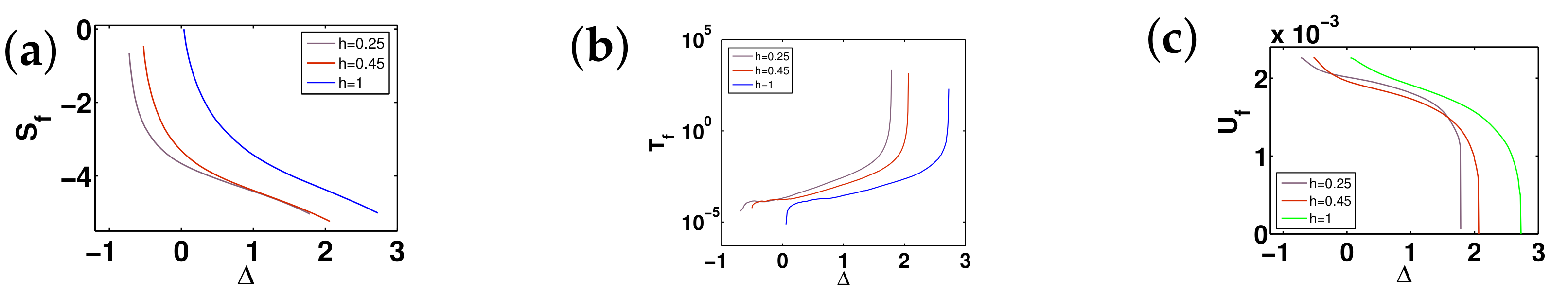
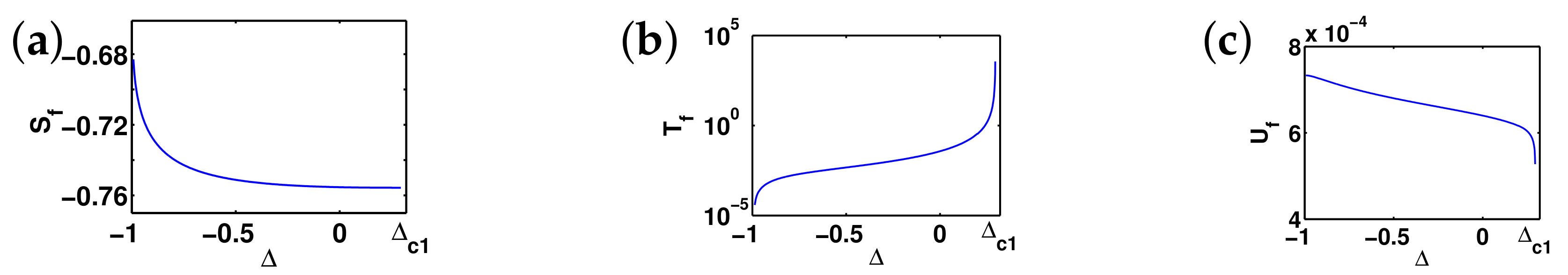
- In part i ( with ), for the chosen dominant control parameter : , the ground-state energy density increases with . Then, from Equation (10), fidelity internal energy takes the following formHere, is an additive constant, and satisfies the singular first-order differential equationwithAccordingly, fidelity temperature follows from
- (2)
- In part iii ( with ), for the chosen dominant control parameter : , the ground-state energy density decreases with . Then, fidelity internal energy takes the following formHere, is an additive constant, and satisfies the singular first-order differential equationwithAccordingly, fidelity temperature follows from
- (3)
- In part v, on the disordered circle, the ground-state energy density is a constant for the chosen dominant control parameter : . Then, fidelity internal energy is a constant, and fidelity temperature is zero:As discussed in Section 2, we have and .
- (a)
- In regime I ( and ), for the chosen dominant control parameter : , the ground-state energy density monotonically decreases with . Then, from Equation (30), fidelity internal energy takes the following formHere, is a function of , and satisfies the singular first-order differential equationwithAccordingly, fidelity temperature in this regime is given by the following
- (b)
- In regime II ( and ), for the chosen dominant control parameter : , the ground-state energy density monotonically increases with . Then, from Equation (30), fidelity internal energy takes the following formHere, is a function of , and satisfies the singular first-order differential equationwithAccordingly, fidelity temperature in this regime is given by the following
- (c)
- (A)
- When a Gaussian critical point is approached, fidelity entropy in part iii and in regime I scale as and , respectively. This indicates that the critical exponent is (cf. Appendix H for details). Combined with a scaling analysis of the ground-state energy density and near a Gaussian critical point : and (cf. Appendix H for details), we have the following:andThe scaling behaviors for part iii and regime I are the same, as anticipated from the fact that they both belong to the Gaussian universality class. Our numerical simulations confirm this scaling analysis.
- (B)
- When an Ising critical point is approached, fidelity entropy in part i, and fidelity entropy , , , and in regime II, regime III, regime IV, and regime V scale as and (, and ). This indicates that the critical exponent is (cf. Appendix H for details). Taking into account the fact that the first-order derivative of and with respect to at a critical point is nonzero, we have the following:andThe scaling behaviors for part i and regimes , with , and , are the same, as anticipated from the fact that they belong to the Ising universality class. Our numerical simulations confirm this scaling analysis.
- (1)
- In part i ( with ), since the integration of with respect to is finite, the singular first-order differential equation, Equation (A46), may be solved as follows:where is a constant to be determined, and takes the following form
- (2)
- (3)
- In part v, simply vanishes, given that is a constant on the disordered circle: .
- (a)
- In regime I ( and ), since the integration of with respect to for a fixed is finite, the singular first-order differential equation, Equation (A55), may be solved as follows:where is a function of , and is defined as follows
- (b)
Appendix K.2. Fidelity Entropy , Fidelity Temperature , and Fidelity Internal Energy : An Interior Point of View
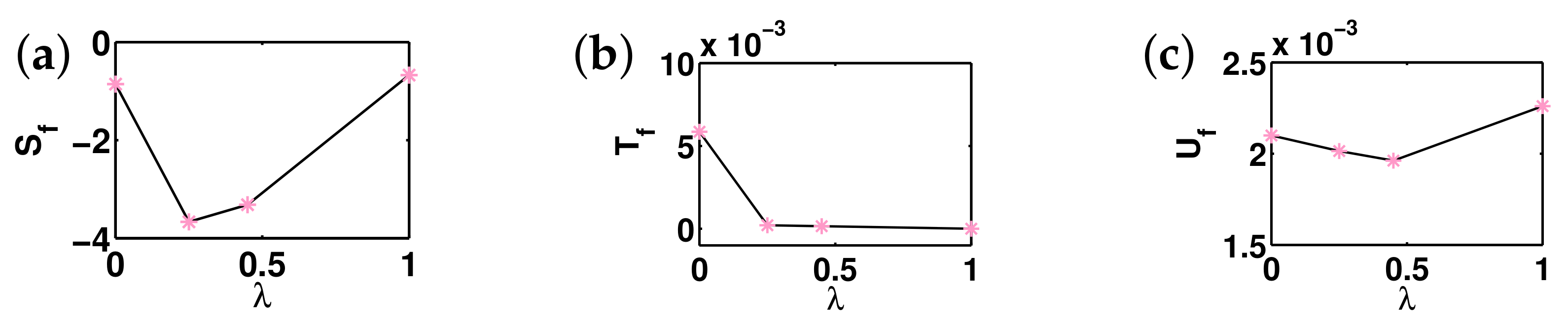
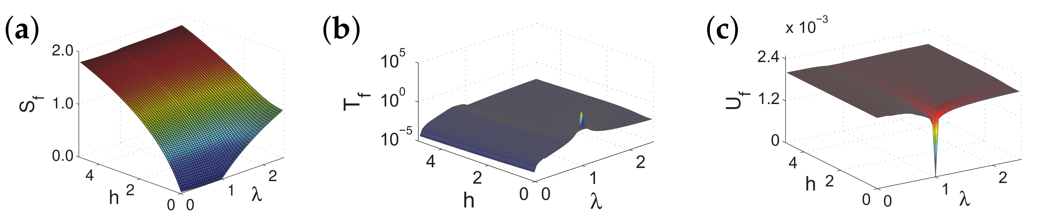
Appendix L. Fidelity Entropy , Fidelity Temperature , and Fidelity Internal Energy for the Transverse-Field Quantum Ising Model in a Longitudinal Field
- (a)
- In regime ( and ), a dominant control parameter was chosen to be and an auxiliary control parameter was chosen to be . In this regime, a re-parametrization operation in the ground-state energy density : is performed, with , to ensure that is monotonic with . Note that if or, equivalently, , then the model reduces to the transverse-field Ising model, which in turn is a special case of the quantum spin- XY model with (cf. Section 7 and Appendix K). As a result, fidelity mechanical-state functions for may be taken from the quantum spin- XY model with (cf. Appendix K). In this Appendix, fidelity mechanical-state functions for the transverse-field Ising model are denoted as , and , with , respectively.
- (b)
- In regime ( and ), a dominant control parameter was chosen to be and an auxiliary control parameter was chosen to be . The ranges of and are and , respectively. In this regime, a re-parametrization operation in the ground-state energy density : , is performed, with . This choice is consistent with the requirement from duality, which occurs when , corresponding to the transverse-field quantum Ising model.

Appendix M. Fidelity Entropy , Fidelity Temperature , and Fidelity Internal Energy for the Quantum Spin- XYZ Model
Appendix M.1. Fidelity Entropy , Fidelity Temperature , and Fidelity Internal Energy : An Exterior Point of View
- (i)
- On the factorizing-field line ( with ), the same factorized state occurs as the ground-state wave function, with the ground-state energy density . We recall that a dominant control parameter was chosen to be for a fixed . Here, a re-parametrization operation in the ground-state energy density : , with , is performed. Therefore, is a constant as varies. Note that the quantum spin- XYZ model becomes the quantum spin- XY model, when . Therefore, fidelity mechanical-state functions for has been determined, as discussed in Appendix K. In particular, fidelity entropy for is known. With this in mind, fidelity entropy on the factorizing-field line ( with ), is identical to up to scaling entropy . Thus, we have . Here, , with . According to our convention (cf. Section 2), we have .
- (ii)
- On the -symmetric line ( with ), we recall that a dominant control parameter was chosen to be . Here, a re-parametrization operation in the ground-state energy density : is performed, with . It should be emphasized that the ground-state energy density is not monotonic as a function of . However, a re-parametrization operation in the ground-state energy density ensures that both and are monotonically decreasing with . In particular, has been chosen to be consistent with duality between regime III and regime IV, (cf. Appendix C). As discussed in Section 2, includes contributions from fidelity entropy and from scaling entropy . That is, , with scaling entropy . Here, takes the following form:where denotes the ground-state fidelity per lattice site in principal part , and is the residual fidelity entropy at the critical point .
- (a)
- In regime ( and ), for the chosen dominant control parameter : , the ground-state energy density monotonically decreases with , for a fixed . Then, from Equation (30), fidelity internal energy takes the formHere, is a function of , and satisfies the singular first-order differential equationwithAccordingly, fidelity temperature in this regime is given by
- (b)

Appendix M.2. Fidelity Entropy , Fidelity Temperature , and Fidelity Internal Energy : An Interior Point of View
Appendix N. Fidelity Entropy, Fidelity Temperature, and Fidelity Internal Energy for the Quantum Spin- XXZ Model in a Magnetic Field
Appendix O. Fidelity Entropy , Fidelity Temperature , and Fidelity Internal Energy for the Quantum Spin-1 XYZ Model
Appendix O.1. Fidelity Entropy , Fidelity Temperature , and Fidelity Internal Energy : An Exterior Point of View

Appendix O.2. Fidelity Entropy , Fidelity Temperature , and Fidelity Internal Energy : An Interior Point of View
Appendix O.3. Fidelity Entropy , Fidelity Temperature , and Fidelity Internal Energy for the Spin-1 Bilinear-Biquadratic Model

Appendix P. Fidelity Entropy , Fidelity Temperature , and Fidelity Internal Energy for the Spin-1/2 Kitaev Model on a Honeycomb Lattice
- (i)
- Regime ( and ): A dominant control parameter was chosen to be , and an auxiliary control parameter was chosen to be .
- (ii)
- Regime (, and ): A dominant control parameter was chosen to be , and an auxiliary control parameter was chosen to be .
Appendix P.1. Fidelity Entropy (, ), Fidelity Temperature (, ), and Fidelity Internal Energy (, ) for the Spin-1/2 Kitaev Model on a Honeycomb Lattice: An Exterior Point of View
Appendix P.2. Fidelity Entropy , Fidelity Temperature , and Fidelity Internal Energy for the Spin-1/2 Kitaev Model on a Honeycomb Lattice: An Interior Point of View
Appendix Q. Zamolodchikov RG Flows vs. Real-Space RG Flows


References
- Sachdev, S. Quantum Phase Transitions; Cambridge University Press: Cambridge, UK, 1999. [Google Scholar]
- Wen, X.-G. Quantum Field Theory of Many-Body Systems; Oxford University Press: Oxford, UK, 2004. [Google Scholar]
- Nishimori, H.; Ortiz, G. Elements of Phase Transitions and Critical Phenomena; Oxford University Press: Oxford, UK, 2011. [Google Scholar]
- Landau, L.D.; Lifshitz, E.M.; Pitaevskii, E.M. Statistical Physics; Butterworth-Heinemann: New York, NY, USA, 1999. [Google Scholar]
- Anderson, P.W. Basic Notions of Condensed Matter Physics, Addison-Wesley: The Advanced Book Program; Addison-Wesley: Reading, MA, USA, 1997. [Google Scholar]
- Coleman, S. An Introduction to Spontaneous Symmetry Breakdown and Gauge Fields: Laws of Hadronic Matter; Academic: New York, NY, USA, 1975. [Google Scholar]
- Kadanoff, L.P. Scaling laws for Ising model near . Physics 1966, 2, 263–272. [Google Scholar] [CrossRef]
- Wilson, K.G. The renormalization group: Critical phenomena and the Kondo problem. Rev. Mod. Phys. 1975, 47, 773–840. [Google Scholar] [CrossRef]
- Fisher, M. The renormalization group in the theory of critical behavior. Rev. Mod. Phys. 1974, 46, 597–616. [Google Scholar] [CrossRef]
- Zinn-Justin, J. Quantum Field Theory and Critical Phenomena; Clarendon Press: Oxford, UK, 2002. [Google Scholar]
- Drell, S.D.; Weinstein, M.; Yankielovicz, S. Quantum field theories on a lattice: Variational methods for arbitrary coupling strengths and the Ising model in a transverse magnetic field. Phys. Rev. D 1977, 16, 1769. [Google Scholar] [CrossRef]
- Jullien, R.; Fields, J.N.; Doniach, S. Kondo Lattice: Real-Space Renormalization-Group Approach. Phys. Rev. Lett. 1977, 38, 1500–1503. [Google Scholar] [CrossRef]
- Wen, X.-G. Topological orders in regid states. Int. J. Mod. Phys. B 1990, 4, 239–271. [Google Scholar] [CrossRef]
- Hasan, M.; Kane, C. Colloquium: Topological insulators. Rev. Mod. Phys. 2010, 82, 3045–3067. [Google Scholar] [CrossRef]
- Qi, X.-L.; Zhang, S.-C. Topological insulators and superconductors. Rev. Mod. Phys. 2011, 83, 1057–1110. [Google Scholar] [CrossRef]
- Zanardi, P.; Paunkovic, N. Ground state overlap and quantum phase transitions. Phys. Rev. E 2006, 74, 031123. [Google Scholar] [CrossRef]
- Zanardi, P.; Cozzini, M.; Giorda, P. Ground state fidelity and quantum phase transitions in free Fermi systems. J. Stat. Mech. Theory Exp. 2007, 2007, L02002. [Google Scholar] [CrossRef] [Green Version]
- Cozzini, M.; Ionicioiu, R.; Zanardi, P. Quantum fidelity and quantum phase transitions in matrix product states. Phys. Rev. B 2007, 76, 104420. [Google Scholar] [CrossRef]
- Venuti, L.C.; Zanardi, P. Quantum critical scaling of the geometric tensors. Phys. Rev. Lett. 2007, 99, 095701. [Google Scholar] [CrossRef] [PubMed]
- You, W.-L.; Li, Y.-W.; Gu, S.-J. Fidelity, dynamic structure factor, and susceptibility in critical phenomena. Phys. Rev. E 2007, 76, 022101. [Google Scholar] [CrossRef] [PubMed]
- Gu, S.-J.; Kwok, H.M.; Ning, W.Q.; Lin, H.-Q. Fidelity susceptibility, scaling, and universality in quantum critical phenomena. Phys. Rev. B 2008, 77, 245109. [Google Scholar] [CrossRef]
- Yang, M.F. Ground-state fidelity in one-dimensional gapless models. Phys. Rev. B 2007, 76, 180403(R). [Google Scholar] [CrossRef]
- Tzeng, Y.C.; Yang, M.F. Scaling properties of fidelity in the spin-1 anisotropic model. Phys. Rev. A 2008, 77, 012311. [Google Scholar] [CrossRef]
- Oelkers, N. Links, Ground-state properties of the attractive one-dimensional Bose-Hubbard model. Phys. Rev. B 2007, 75, 115119. [Google Scholar] [CrossRef]
- Fjaerestad, J.O. Ground state fidelity of Luttinger liquids: A wavefunctional approach. J. Stat. Mech. Theory Exp. 2008, 2008, P07011. [Google Scholar] [CrossRef]
- Zhou, H.-Q.; Barjaktarevic, J.P. Fidelity and quantum phase transitions. J. Phys. A Math. Theor. 2008, 41, 412001. [Google Scholar] [CrossRef]
- Zhou, H.-Q.; Zhao, J.-H.; Li, B. Fidelity approach to quantum phase transitions: Finite-size scaling for the quantum Ising model in a transverse field. J. Phys. A Math. Theor. 2008, 41, 492002. [Google Scholar] [CrossRef]
- Zhou, H.-Q.; Orús, R.; Vidal, G. Ground State Fidelity from Tensor Network Representations. Phys. Rev. Lett. 2008, 100, 080601. [Google Scholar] [CrossRef] [PubMed]
- Zhao, J.-H.; Zhou, H.-Q. Singularities in ground-state fidelity and quantum phase transitions for the Kitaev model. Phys. Rev. B 2009, 80, 014403. [Google Scholar] [CrossRef]
- Wang, H.-L.; Zhao, J.-H.; Li, B.; Zhou, H.-Q. Kosterlitz-Thouless phase transition and ground state fidelity: A novel perspective from matrix product states. J. Stat. Mech. 2011, 2011, L10001. [Google Scholar] [CrossRef]
- Kitaev, A. Anyons in an exactly solved model and beyond. Ann. Phys. 2006, 321, 2–111. [Google Scholar] [CrossRef]
- Baskaran, G.; Mandal, S.; Shankar, R. Exact results for spin dynamics and fractionalization in the Kitaev model. Phys. Rev. Lett. 2007, 98, 247201. [Google Scholar] [CrossRef] [PubMed]
- Chen, H.-D.; Nussinov, Z. Exact results of the Kitaev model on a hexagonal lattice: Spin states, string and brane correlators, and anyonic excitations. J. Phys. A Math. Theor. 2008, 41, 075001. [Google Scholar] [CrossRef]
- Berezinskii, V.L. Destruction of long range order in one dimensional and two dimensional systems having a continuous symmetry group I. classical systems. Sov. Phys. JETP 1972, 34, 610–616. [Google Scholar]
- Kosterlitz, J.M.; Thouless, D.J. Ordering, metastability and phase transitions in two-dimensional systems. J. Phys. C Solid State Phys. 1973, 6, 1181–1203. [Google Scholar] [CrossRef]
- Nielsen, M.A.; Chuang, I.L. Quantum Computation and Quantum Information; Cambridge University Press: Cambridge, UK, 2000. [Google Scholar]
- White, S.R. Density matrix formulation for quantum renormalization groups. Phys. Rev. Lett. 1992, 69, 2863–2866. [Google Scholar] [CrossRef]
- Schollwöck, U. The density-matrix renormalization group. Rev. Mod. Phys. 2005, 77, 259–315. [Google Scholar] [CrossRef]
- Verstraete, F.; Cirac, J.I.; Murg, V. Matrix product states, projected entangled pair states, and variational renormalization group methods for quantum spin systems. Adv. Phys. 2008, 57, 143–224. [Google Scholar] [CrossRef] [Green Version]
- Cirac, J.I.; Verstraete, F.J. Renormalization and tensor product states in spin chains and lattices. J. Phys. A Math. Theor. 2009, 42, 504004. [Google Scholar] [CrossRef]
- Jordan, J.; Orús, R.; Vidal, G.; Verstraete, F.; Cirac, J.I. Classical simulation of infinite-size quantum lattice systems in two spatial dimensions. Phys. Rev. Lett. 2008, 101, 250602. [Google Scholar] [CrossRef] [PubMed]
- Shi, Q.-Q.; Li, S.-H.; Zhao, J.-H.; Zhou, H.-Q. Graded projected entangled-pair state representations and an algorithm for translationally invariant strongly correlated electronic systems on infinite-size lattices in two spatial dimensions. arXiv 2009, arXiv:0907.5520. [Google Scholar]
- Li, S.-H.; Shi, Q.-Q.; Zhou, H.-Q. Ground-state phase diagram of the two-dimensional t-J model. arXiv 2010, arXiv:1001.3343. [Google Scholar]
- Kraus, C.V.; Schuch, N.; Verstraete, F.; Cirac, J.I. Fermionic projected entangled pair states. Phys. Rev. A 2010, 81, 052338. [Google Scholar] [CrossRef]
- Piˇzorn, I.; Verstraete, F. Fermionic implementation of projected entangled pair states algorithm. Phys. Rev. B 2010, 81, 245110. [Google Scholar] [CrossRef]
- Vidal, G. Efficient classical simulation of slightly entangled quantum computations. Phys. Rev. Lett. 2003, 91, 147902. [Google Scholar] [CrossRef]
- Vidal, G. Efficient simulation of one-dimensional quantum many-body systems. Phys. Rev. Lett. 2004, 93, 040502. [Google Scholar] [CrossRef]
- Vidal, G. Classical simulation of infinite-size quantum lattice systems in one spatial dimension. Phys. Rev. Lett. 2007, 98, 070201. [Google Scholar] [CrossRef]
- Zhou, H.-Q. Deriving local order parameters from tensor network representations. arXiv 2008, arXiv:0803.0585. [Google Scholar]
- Li, S.-H.; Shi, Q.-Q.; Su, Y.-H.; Liu, J.-H.; Dai, Y.-W.; Zhou, H.-Q. Tensor network states and ground-state fidelity for quantum spin ladders. Phys. Rev. B 2012, 86, 064401. [Google Scholar] [CrossRef]
- Laughlin, R.B.; Pines, D. The theory of everything. Proc. Natl. Acad. Sci. USA 2000, 97, 28–31. [Google Scholar] [CrossRef] [PubMed]
- Zamolodchikov, A.B. “Irreversibility” of the flux of the renormalization group in a 2D field theory. JETP Lett. 1986, 43, 730–732. [Google Scholar]
- Cardy, J. Scaling and Renormalization in Statistical Physics; Cambridge University Press: Cambridge, UK, 1996. [Google Scholar]
- Francesco, P.D.; Mathieu, P.; Sénxexchal, D. Conformal Field Theory; Springer: Berlin/Heidelberg, Germany, 1997. [Google Scholar]
- Cardy, J. The ubiquitous ‘c’: From the Stefan-Boltzmann law to quantum information. J. Stat. Mech. 2010, 2010, P10004. [Google Scholar] [CrossRef] [Green Version]
- Komargodski, Z.; Schwimmer, A. On renormalization group flows in four dimensions. J. High Energy Phys. 2011, 12, 99. [Google Scholar] [CrossRef]
- Gaite, J.; O’Connor, D. Field theory entropy, the H theorem, and the renormalization group. Phys. Rev. D 1996, 54, 5163–5173. [Google Scholar] [CrossRef]
- Landauer, R. Irreversibility and heat generation in the computing process. IBM J. Res. Dev. 1961, 5, 183–191. [Google Scholar] [CrossRef]
- Wolf, M.M.; Ortiz, G.; Verstraete, F.; Cirac, J.I. Quantum phase transitions in matrix product systems. Phys. Rev. Lett. 2006, 97, 110403. [Google Scholar] [CrossRef]
- Amico, L.; Fazio, R.; Osterloh, A.; Vedral, V. Entanglement in many-body systems. Rev. Mod. Phys. 2008, 80, 517–576. [Google Scholar] [CrossRef]
- Kitaev, A.; Preskill, J. Topological entanglement entropy. Phys. Rev. Lett. 2006, 96, 110404. [Google Scholar] [CrossRef] [PubMed]
- Levin, M.; Wen, X.-G. Detecting topological order in a ground state wave function. Phys. Rev. Lett. 2006, 96, 110405. [Google Scholar] [CrossRef] [PubMed]
- Dzhaparidze, G.I.; Nersesyan, A.A. Magnetic-field phase transition in a one-dimensional system of electrons with attraction. JETP Lett. 1978, 27, 334–337. [Google Scholar]
- Pokrovsky, V.L.; Talapov, A.L. Ground State, spectrum, and phase diagram of two-dimensional incommensurate crystals. Phys. Rev. Lett. 1979, 42, 65–67. [Google Scholar] [CrossRef]
- Haldane, F.D.M. Continuum dynamics of the 1-D Heisenberg antiferromagnet: Identification with the O(3) nonlinear sigma model. Phys. Lett. A 1983, 93, 464–468. [Google Scholar] [CrossRef]
- Haldane, F.D.M. Nonlinear field theory of large-spin Heisenberg antiferromagnets: Semiclassically quantized solitons of the one-dimensional easy-axis néel state. Phys. Rev. Lett. 1983, 50, 1153. [Google Scholar] [CrossRef]
- McCulloch, I.P. Infinite size density matrix renormalization group, revisited. arXiv 2008, arXiv:0804.2509. [Google Scholar]
- McCulloch, I.P. From density-matrix renormalization group to matrix product states. J. Stat. Mech. 2007, 2007, P10014. [Google Scholar] [CrossRef]
- Peters, D.; McCulloch, I.P.; Selke, W. Ground-state properties of antiferromagnetic anisotropic S = 1 Heisenberg spin chains. Phys. Rev. B 2012, 85, 054423. [Google Scholar] [CrossRef]
- Huang, C.-Y.; Lin, F.-L. Quantum key distribution over probabilistic quantum repeaters. Phys. Rev. A 2010, 81, 032304. [Google Scholar] [CrossRef]
- Shi, Q.-Q.; Wang, H.-L.; Li, S.-H.; Cho, S.Y.; Batchelor, M.T.; Zhou, H.-Q. Geometric entanglement and quantum phase transitions in two-dimensional quantum lattice models. Phys. Rev. A 2016, 93, 062341. [Google Scholar] [CrossRef]
- Papadimitriou, C.H. Computational Complexity; Addison-Wesley: Boston, MA, USA, 1994. [Google Scholar]
- Li, B.; Li, S.-H.; Zhou, H.-Q. Quantum phase transitions in a two-dimensional quantum XYX model: Ground-state fidelity and entanglement. Phys. Rev. E 2009, 79, 060101R. [Google Scholar] [CrossRef] [PubMed]
- Wang, H.-L.; Dai, Y.-W.; Hu, B.-Q.; Zhou, H.-Q. Bifurcation in ground-state fidelity for a one-dimensional spin model with competing two-spin and three-spin interactions. Phys. Lett. A 2011, 375, 4045–4048. [Google Scholar] [CrossRef]
- Wang, H.-L.; Chen, A.-M.; Li, B.; Zhou, H.-Q. Ground-state fidelity and Kosterlitz-Thouless phase transition for the spin-1/2 Heisenberg chain with next-to-the-nearest-neighbor interaction. J. Phys. A Math. Theor. 2012, 45, 015306. [Google Scholar] [CrossRef]
- Kramers, H.A.; Wannier, G.H. Statistics of the two-dimensional ferromagnet. Part I. Phys. Rev. 1941, 60, 252–262. [Google Scholar]
- Giampaolo, S.M.; Adesso, G.; Illuminati, F. Theory of ground state factorization in quantum cooperative systems. Phys. Rev. Lett. 2008, 100, 197201. [Google Scholar] [CrossRef]
- Giampaolo, S.M.; Adesso, G.; Illuminati, F. Separability and ground-state factorization in quantum spin systems. Phys. Rev. B 2009, 79, 224434. [Google Scholar] [CrossRef]
- Giampaolo, S.M.; Adesso, G.; Illuminati, F. Probing quantum frustrated systems via factorization of the ground state. Phys. Rev. Lett. 2010, 104, 207202. [Google Scholar] [CrossRef] [Green Version]
- Kurmann, J.; Thomas, H.; Muller, G. Antiferromagnetic long-range order in the anisotropic quantum spin chain. Phys. A 1982, 112, 235–255. [Google Scholar] [CrossRef]
- Roscilde, T.; Verrucchi, P.; Fubini, A.; Haas, S.; Tognetti, V. Studying quantum spin systems through entanglement estimators. Phys. Rev. Lett. 2004, 93, 167203. [Google Scholar] [CrossRef]
- Roscilde, T.; Verrucchi, P.; Fubini, A.; Haas, S.; Tognetti, V. Entanglement and factorized ground states in two-dimensional quantum antiferromagnets. Phys. Rev. Lett. 2005, 94, 147208. [Google Scholar] [CrossRef] [PubMed]
- Messiah, A. Quantum Mechanics; John Wiley and Sons: Hoboken, NJ, USA, 1966; Volumes I–II. [Google Scholar]
- Berry, M. Transitionless quantum driving. J. Phys. A Math. Theor. 2009, 42, 365303. [Google Scholar] [CrossRef]
- Campo, A.D.; Rams, M.M.; Zurek, W.H. Assisted finite-rate adiabatic passage across a quantum critical point: Exact solution for the quantum Ising model. Phys. Rev. Lett. 2012, 109, 115703. [Google Scholar] [CrossRef] [PubMed]
- Vaas, R. Time After Time-Big Bang Cosmology and the Arrows of Time. In The Arrows of Time, Fundamental Theories of Physics; Mersini-Houghton, L., Vaas, R., Eds.; Springer: Berlin/Heidelberg, Germany, 2012; Volume 172. [Google Scholar]
- Anderson, P.W. More is different: Broken symmetry and the nature of the hierarchical structure of science. Science 1972, 177, 393. [Google Scholar] [CrossRef] [PubMed]
- Kroemer, H.; Kittel, C. Thermal Physics, 2nd ed.; W. H. Freeman Company: New York, NY, USA, 1980. [Google Scholar]
- Kibble, T.W.B. Topology of cosmic domains and strings. J. Phys. A Math. Gen. 1976, 9, 1387. [Google Scholar] [CrossRef]
- Kibble, T.W.B. Some implications of a cosmological phase transition. Phys. Rep. 1980, 67, 183–199. [Google Scholar] [CrossRef]
- Zurek, W.H. Cosmological experiments in superfluid helium? Nature 1985, 317, 505–508. [Google Scholar] [CrossRef]
- Zurek, W.H. Cosmological experiments in condensed matter systems. Phys. Rep. 1996, 276, 177–221. [Google Scholar] [CrossRef] [Green Version]
- Damski, B. The simplest quantum model supporting the Kibble-Zurek mechanism of topological defect production: Landau-Zener transitions from a new perspective. Phys. Rev. Lett. 2005, 95, 035701. [Google Scholar] [CrossRef]
- Zurek, W.H.; Dorner, U.; Zoller, P. Dynamics of a quantum phase transition. Phys. Rev. Lett. 2005, 95, 105701. [Google Scholar] [CrossRef]
- Dziarmaga, J. Dynamics of a quantum phase transition: Exact solution of the quantum Ising model. Phys. Rev. Lett. 2005, 95, 245701. [Google Scholar] [CrossRef] [PubMed]
- Osborne, T.J.; Nielsen, M.A. Entanglement in a simple quantum phase transition. Phys. Rev. A 2002, 66, 032110. [Google Scholar] [CrossRef]
- Osterloh, A.; Amico, L.; Falci, G.; Fazio, R. Scaling of entanglement close to a quantum phase transition. Nature 2002, 416, 608–610. [Google Scholar] [CrossRef]
- Hawking, S.W. Particle creation by black holes. Commun. Math. Phys. 1975, 43, 199–220. [Google Scholar] [CrossRef]
- Hawking, S.W. Black Hole Explosions? Nature 1974, 248, 30–31. [Google Scholar] [CrossRef]
- Jiang, H.-C.; Gu, Z.-C.; Qi, X.-L.; Trebst, S. Possible proximity of the Mott insulating iridate Na2IrO3 to a topological phase: Phase diagram of the Heisenberg-Kitaev model in a magnetic field. Phys. Rev. B 2011, 83, 245104. [Google Scholar] [CrossRef]
- Gohlke, M.; Moessner, R.; Pollmann, F. Dynamical and topological properties of the Kitaev model in a [111] magnetic field. Phys. Rev. B 2018, 98, 014418. [Google Scholar] [CrossRef]
- Shi, Q.-Q.; Dai, Y.-W.; Zhou, H.-Q.; McCulloch, I. Fractal dimension and the counting rule of the Goldstone modes. arXiv 2022, arXiv:2201.01071. [Google Scholar]
- Mermin, N.D.; Wagner, H. Absence of ferromagnetism or antiferromagnetism in one- or two-dimensional isotropic Heisenberg models. Phys. Rev. Lett. 1966, 17, 1133. [Google Scholar] [CrossRef]
- Coleman, S.R. There are no Goldstone bosons in two dimensions. Commun. Math. Phys. 1973, 31, 259–264. [Google Scholar] [CrossRef]
- Watanabe, H.; Murayama, H. Unified description of Nambu-Goldstone bosons without Lorentz invariance. Phys. Rev. Lett. 2012, 108, 251602. [Google Scholar] [CrossRef] [PubMed]
- Hidaka, Y. Counting rule for Nambu-Goldstone modes in nonrelativistic systems. Phys. Rev. Lett. 2013, 110, 091601. [Google Scholar] [CrossRef] [PubMed]
- Berry, M. Singular limits. Phys. Today 2002, 55, 10–11. [Google Scholar] [CrossRef]
- Chen, X.; Gu, Z.-C.; Wen, X.-G. Classification of gapped symmetric phases in one-dimensional spin systems. Phys. Rev. B 2011, 83, 0355107. [Google Scholar] [CrossRef]
- Chen, X.; Gu, Z.-C.; Wen, X.-G. Complete classification of one-dimensional gapped quantum phases in interacting spin systems. Phys. Rev. B 2011, 84, 235128. [Google Scholar] [CrossRef]
- Pollmann, F.; Turner, A.M.; Berg, E.; Oshikawa, M. Entanglement spectrum of a topological phase in one dimension. Phys. Rev. B 2010, 81, 064439. [Google Scholar] [CrossRef]
- Rao, W.-J.; Zhu, G.-Y.; Zhang, G.-M. SU(3) quantum critical model emerging from a spin-1 topological phase. Phys. Rev. B 2016, 93, 165135. [Google Scholar] [CrossRef]
- Pollmann, F.; Turner, A.M. Detection of symmetry-protected topological phases in one dimension. Phys. Rev. B 2012, 86, 125441. [Google Scholar] [CrossRef]
- Fuji, Y.; Pollmann, F.; Oshikawa, M. Distinct trivial phases protected by a point-group symmetry in quantum spin chains. Phys. Rev. Lett. 2015, 114, 177204. [Google Scholar] [CrossRef] [Green Version]
- Chen, X.-H.; McCulloch, I.; Batchelor, M.T.; Zhou, H.-Q. Symmetry-protected trivial phases and quantum phase transitions in an anisotropic antiferromagnetic spin-1 biquadratic model. Phys. Rev. B 2020, 102, 085146. [Google Scholar] [CrossRef]
- Pollmann, F.; Berg, E.; Turner, A.M.; Oshikawa, M. Symmetry protection of topological phases in one-dimensional quantum spin systems. Phys. Rev. B 2012, 85, 075125. [Google Scholar] [CrossRef]
- Lieb, E.; Schultz, T.; Mattis, D. Two soluble models of an antiferromagnetic chain. Ann. Phys. 1961, 16, 407–466. [Google Scholar] [CrossRef]
- Lieb, E.; Mattis, D. Mathematical Physics in One Dimension; Academic Press: New York, NY, USA; London, UK, 1966. [Google Scholar]
- Pfeuty, P. The one-dimensional Ising model with a transverse field. Ann. Phys. 1970, 57, 79–90. [Google Scholar] [CrossRef]
- Giampaolo, S.M.; Montangero, S.; Anno, F.D.; Siena, S.D.; Illuminati, F. Universal aspects in the behavior of the entanglement spectrum in one dimension: Scaling transition at the factorization point and ordered entangled structures. Phys. Rev. B 2013, 88, 125142. [Google Scholar] [CrossRef]
- Franchini, F.; Its, A.R.; Jin, B.-Q.; Korepin, V.E. Ellipses of constant entropy in the XY spin chain. J. Phys. A Math. Theor. 2007, 40, 8467. [Google Scholar] [CrossRef]
- Zamolodchikov, A.B. Integrable field theory from conformal field theory. Adv. Stud. Pure Math. 1989, 19, 641–674. [Google Scholar]
- Baxter, R.J. One-Dimensional anisotropic Heisenberg chain. Phys. Rev. Lett. 1971, 26, 834. [Google Scholar] [CrossRef]
- Baxter, R.J. Eight-Vertex Model in Lattice Statistics. Phys. Rev. Lett. 1971, 26, 832–833. [Google Scholar] [CrossRef]
- Baxter, R.J. Partition function of the Eight-Vertex lattice model. Ann. Phys. 1972, 70, 193–228. [Google Scholar] [CrossRef]
- Baxter, R.J. Exactly Solved Models in Statistical Mechanics; Academic Press: Cambridge, MA, USA, 1982. [Google Scholar]
- Faddeev, L.D.; Takhtadzhyan, L.A. Spectrum and scattering of excitations in the one-dimensional isotropic Heisenberg model. J. Math. Sci. 1984, 24, 241–267. [Google Scholar] [CrossRef]
- Korepin, V.E.; Bogoliubov, N.M.; Izergin, A.G. Quantum Inverse Scattering Method and Correlation Functions; Cambridge University Press: Cambridge, UK, 1996. [Google Scholar]
- Cloizeaux, J.; Gaudin, M. Anisotropic Linear Magnetic Chain. J. Math. Phys. 1966, 7, 1384–1400. [Google Scholar] [CrossRef]
- Yang, C.N.; Yang, C.P. Thermodynamics of a one-dimensional system of bosons with repulsive delta-function interaction. J. Math. Phys. 1969, 10, 1115–1122. [Google Scholar] [CrossRef]
- Luther, A.; Peschel, I. Calculation of critical exponents in two dimensions from quantum field theory in one dimension. Phys. Rev. B 1975, 12, 3908–3917. [Google Scholar] [CrossRef]
- Essler, F.H.L.; Konik, R.M. From Fields to Strings: Circumnavigating Theoretical Physics; World Scientific: Singapore, 2005; pp. 684–830. [Google Scholar]
- Cabra, D.C.; Honecker, A.; Pujol, P. Magnetization plateaux in N-leg spin ladders. Phys. Rev. B 1998, 58, 6241–6257. [Google Scholar] [CrossRef]
- Affleck, I.; Kennedy, T.; Lieb, E.H.; Tasaki, H. Rigorous results on valence-bond ground states in antiferromagnets. Phys. Rev. Lett. 1987, 59, 799. [Google Scholar] [CrossRef] [PubMed]
- Affleck, I.; Kennedy, T.; Lieb, E.H.; Tasaki, H. Valence bond ground states in isotropic quantum antiferromagnets. Commun. Math. Phys. 1988, 115, 477–528. [Google Scholar] [CrossRef]
- Chubukov, A.V. Spontaneous dimerization in quantum-spin chains. Phys. Rev. B 1991, 43, 3337–3344. [Google Scholar] [CrossRef]
- Fáth, G.; Sólyom, J. Search for the nondimerized quantum nematic phase in the spin-1 chain. Phys. Rev. B 1995, 51, 3620–3625. [Google Scholar] [CrossRef] [PubMed]
- Kawashima, N. Quantum monte carlo methods. Prog. Theor. Phys. Suppl. 2002, 145, 138–149. [Google Scholar] [CrossRef]
- Ivanov, B.A.; Kolezhuk, A.K. Effective field theory for the S = 1 quantum nematic. Phys. Rev. B 2003, 68, 052401. [Google Scholar] [CrossRef] [Green Version]
- Buchta, K.; Fáth, G.; Legeza, O.; Sólyom, J. Probable absence of a quadrupolar spin-nematic phase in the bilinear-biquadratic spin-1 chain. Phys. Rev. B 2005, 72, 054433. [Google Scholar] [CrossRef]
- Rizzi, M.; Rossini, D.; Chiara, G.D.; Montangero, S.; Fazio, R. Phase diagram of spin-1 bosons on one-dimensional lattices. Phys. Rev. Lett. 2005, 95, 240404. [Google Scholar] [CrossRef] [PubMed]
- Läuchli, A.; Schmid, G.; Trebst, S. Spin nematics correlations in bilinear-biquadratic S = 1 spin chains. Phys. Rev. B 2006, 74, 144426. [Google Scholar] [CrossRef]
- Porras, D.; Verstraete, F.; Cirac, J.I. Renormalization algorithm for the calculation of spectra of interacting quantum systems. Phys. Rev. B 2006, 73, 014410. [Google Scholar] [CrossRef]
- Romero-Isart, O.; Eckert, K.; Sanpera, A. Quantum state transfer in spin-1 chains. Phys. Rev. A 2007, 75, 050303(R). [Google Scholar] [CrossRef]
- Rakov, M.V.; Weyrauch, M. Bilinear-biquadratic spin-1 rings: An SU(2)-symmetric MPS algorithm for periodic boundary conditions. J. Phys. Commun. 2017, 1, 015007. [Google Scholar] [CrossRef]
- Cirac, J.I.; Sierra, G. Infinite matrix product states, conformal field theory, and the Haldane-Shastry model. Phys. Rev. B 2010, 81, 104431. [Google Scholar] [CrossRef]
- Nielsen, A.E.B.; Cirac, J.I.; Sierra, G. Quantum spin Hamiltonians for the SU(2)k WZW model. J. Stat. Mech. 2011, 2011, P11014. [Google Scholar] [CrossRef]
- Fáth, G.; Sólyom, J. Period tripling in the bilinear-biquadratic antiferromagnetic S = 1 chain. Phys. Rev. B 1991, 44, 11836–11844. [Google Scholar] [CrossRef]
- Sutherland, B. Model for a multicomponent quantum system. Phys. Rev. B 1975, 12, 3795–3805. [Google Scholar] [CrossRef]
- Barber, M.N.; Batchelor, M.T. Spectrum of the biquadratic spin-1 antiferromagnetic chain. Phys. Rev. B 1989, 40, 4621–4626. [Google Scholar] [CrossRef] [PubMed]
- Batista, C.D.; Ortiz, G.; Gubernatis, J.E. Unveiling order behind complexity: Coexistence of ferromagnetism and Bose-Einstein condensation. Phys. Rev. B 2002, 65, 180402(R). [Google Scholar] [CrossRef]
- Affleck, I.J. Exact results on the dimerisation transition in SU(n) antiferromagnetic chains. Phys. Condens. Matter 1990, 2, 405–415. [Google Scholar] [CrossRef]
- Takhtajan, L. The picture of low-lying excitations in the isotropic Heisenberg chain of arbitrary spins. Phys. Lett. A 1982, 87, 479–482. [Google Scholar] [CrossRef]
- Babujian, H. Exact solution of the isotropic Heisenberg chain with arbitrary spins: Thermodynamics of the model. Nucl. Phys. B 1983, 215, 317–336. [Google Scholar] [CrossRef]
- Batchelor, M.T.; Barber, M.N. Spin-s quantum chains and Temperley-Lieb algebras. J. Phys. A Math. Gen. 1990, 23, L15. [Google Scholar] [CrossRef]
- Aufgebauer, B.; Kluemper, A. Quantum spin chains of Temperley-Lieb type: Periodic boundary conditions, spectral multiplicities and finite temperature. J. Stat. Mech. 2010, 2010, P05018. [Google Scholar] [CrossRef]
- Lundgren, R.; Blair, J.; Laurell, P.; Regnault, N.; Fiete, G.A.; Greiter, M.; Thomale, R. Universal entanglement spectra in critical spin chains. Phys. Rev. B 2016, 94, 081112. [Google Scholar] [CrossRef]
- Thomale, R.; Rachel, S.; Bernevig, B.A.; Arovas, D.P. Entanglement analysis of isotropic spin-1 chains. J. Stat. Mech. 2015, 2015, P07017. [Google Scholar] [CrossRef]
- Dai, Y.-W.; Shi, Q.-Q.; Zhou, H.-Q.; McCulloch, I. Absence of a critical nematic phase in the vicinity of the SU(3) ferromagnetic point for the one-dimensional spin-1 bilinear-biquadratic model. arXiv 2022, arXiv:2201.01434. [Google Scholar]
- den Nijs, M.; Rommelse, K. Preroughening transitions in crystal surfaces and valence-bond phases in quantum spin chains. Phys. Rev. B 1989, 40, 4709. [Google Scholar] [CrossRef] [PubMed]
- Kennedy, T.; Tasaki, H. Hidden Z2 × Z2 symmetry breaking in Haldane-gap antiferromagnets. Phys. Rev. B 1992, 45, 304–308. [Google Scholar] [CrossRef] [PubMed]
- Oshikawa, M. Hidden Z2 × Z2 symmetry in quantum spin chains with arbitrary integer spin. J. Phys. Condens. Matter 1992, 4, 7469–7488. [Google Scholar] [CrossRef]
- Boschi, C.D.E.; Ercolessi, E.; Ortolani, F.; Roncaglia, M. On c = 1 critical phases in anisotropic spin-1 chains. Eur. Phys. J. B 2003, 35, 465–473. [Google Scholar] [CrossRef]
- Ueda, H.; Nakano, H.; Kusakabe, K. Finite-size scaling of string order parameters characterizing the Haldane phase. Phys. Rev. B 2008, 78, 224402. [Google Scholar] [CrossRef]
- Micheli, A.; Brennen, G.K.; Zoller, P. A toolbox for lattice-spin models with polar molecules. Nat. Phys. 2006, 2, 341–347. [Google Scholar] [CrossRef]
- Feng, X.-Y.; Zhang, G.-M.; Xiang, T. Topological characterization of quantum phase transitions in a spin-1/2 model. Phys. Rev. Lett. 2007, 98, 087204. [Google Scholar] [CrossRef]
- Cui, J.; Cao, J.-P.; Fan, H. Quantum-Information approach to the quantum phase transition in the Kitaev honeycomb model. Phys. Rev. A 2010, 82, 022319. [Google Scholar] [CrossRef]
- Bardeen, J.M.; Carter, B.; Hawking, S. The four laws of black hole mechanics. Commun. Math. Phys. 1973, 31, 161–170. [Google Scholar] [CrossRef]
- Spergel, D.N. Cosmology today. Daedalus Am. Acad. Arts Sci. 2014, 143, 125–133. [Google Scholar] [CrossRef]
- Gough, M.P. Information equation of state. Entropy 2008, 10, 150–159. [Google Scholar] [CrossRef] [Green Version]
- Gough, M.P. Holographic dark information energy. Entropy 2011, 13, 924–935. [Google Scholar] [CrossRef]
- Gough, M.P. Holographic dark information energy: Predicted dark energy measurement. Entropy 2013, 15, 1135–1151. [Google Scholar] [CrossRef]
- Gough, M.P. A dynamic dark information energy consistent with planck data. Entropy 2014, 16, 1902–1916. [Google Scholar] [CrossRef]
- Gogolin, A.O.; Nersesyan, A.A.; Tsvelik, A.M. Bosonization and Strongly Correlated Systems; Cambridge University Press: Cambridge, UK, 1998. [Google Scholar]
- Rao, S.; Sen, D. An introduction to bosonization and some of its applications. In Field Theories in Condensed Matter Systems; Rao, S., Ed.; Hindustan Book Agency: New Delhi, India, 2001. [Google Scholar]
- Shi, Q.-Q.; Dai, Y.-W.; Li, S.-H.; Zhou, H.-Q. Instability of the Luttinger liquids towards an exotic quantum state of matter with highly degenerate ground states: An anisotropic extension of the ferromagnetic spin-1 biquadratic model. arXiv 2022, arXiv:2204.05692. [Google Scholar]
- Watanabe, H.; Brauner, T.; Murayama, H. Massive Nambu-Goldstone bosons. Phys. Rev. Lett. 2013, 111, 021601. [Google Scholar] [CrossRef] [PubMed]
- Hayata, T.; Hidaka, Y. Dispersion relations of Nambu-Goldstone modes at finite temperature and density. Phys. Rev. D 2015, 91, 056006. [Google Scholar] [CrossRef]
- Takahashi, D.A.; Nitta, M. Counting rule of Nambu-Goldstone modes for internal and spacetime symmetries: Bogoliubov theory approach. Ann. Phys. 2015, 354, 101–156. [Google Scholar] [CrossRef]
- Nambu, Y. Spontaneous breaking of Lie and current algebras. J. Stat. Phys. 2004, 115, 7–17. [Google Scholar] [CrossRef]
- Watanabe, H.; Brauner, T. Number of Nambu-Goldstone bosons and its relation to charge densities. Phys. Rev. D 2011, 84, 125013. [Google Scholar] [CrossRef]
- Watanabe, H.; Murayama, H. Effective Lagrangian for Nonrelativistic Systems. Phys. Rev. X 2014, 4, 031057. [Google Scholar] [CrossRef]
- Schafer, T.; Son, D.T.; Stephanov, M.A.; Toublan, D.; Verbaarschot, J.J.M. Kaon condensation and Goldstone’s theorem. Phys. Lett. B 2001, 522, 67–75. [Google Scholar] [CrossRef] [Green Version]
- Miransky, V.A.; Shovkovy, I.A. Spontaneous symmetry breaking with abnormal number of Nambu-Goldstone bosons and kaon condensate. Phys. Rev. Lett. 2002, 88, 111601. [Google Scholar] [CrossRef] [PubMed]
- Nicolis, A.; Piazza, F. Implications of relativity on nonrelativistic Goldstone theorems: Gapped excitations at finite charge density. Phys. Rev. Lett. 2013, 110, 011602. [Google Scholar] [CrossRef] [PubMed]
- Beekman, A.J.; Rademaker, L.; van Wezel, J. An introduction to spontaneous symmetry breaking. SciPost Phys. Lect. Notes 2019, 11, 1–140. [Google Scholar] [CrossRef]
- Castro-Alvaredo, O.A.; Doyon, B.J. Permutation operators, entanglement entropy, and the XXZ spin chain in the limit Δ → −1+. J. Stat. Mech. 2011, 1102, P02001. [Google Scholar] [CrossRef]
- Castro-Alvaredo, O.A.; Doyon, B. Entanglement entropy of highly degenerate states and fractal dimensions. Phys. Rev. Lett. 2012, 108, 120401. [Google Scholar] [CrossRef]
- Popkov, V.; Salerno, M. Logarithmic divergence of the block entanglement entropy for the ferromagnetic Heisenberg model. Phys. Rev. A 2005, 71, 012301. [Google Scholar] [CrossRef]
- Popkov, V.; Salerno, M.; Schütz, G. Entangling power of permutation-invariant quantum states. Phys. Rev. A 2005, 72, 032327. [Google Scholar] [CrossRef]
- Temperley, H.N.V.; Lieb, E.H. Relations between ‘percolation’ and ‘colouring’ problems and other graph theoretical problems associated with regular planar lattices: Some exact results for the percolation problem. Proc. R. Soc. Lond. A 1971, 322, 251–280. [Google Scholar]
- Martin, P. Potts Models and Related Problems in Statistical Mechanics; World Scientific: Singapore, 1991. [Google Scholar]
- Jones, V.F.R. Index for subfactors. Invent. Math. 1983, 72, 1–25. [Google Scholar] [CrossRef]
- Pasquier, V. Two-dimensional critical systems labelled by Dynkin diagrams. Nucl. Phys. B 1987, 285, 162–172. [Google Scholar] [CrossRef]
- Wenzl, H. Hecke algebras of type An and subfactors. Invent. Math. 1988, 92, 349–383. [Google Scholar] [CrossRef]
- Kuniba, A.; Akutsu, Y.; Wadati, M. Virasoro Algebra, von Neumann algebra and critical eight-vertex SOS models. J. Phys. Soc. Jpn. 1986, 55, 3285–3288. [Google Scholar] [CrossRef]
- Andrews, G.E.; Baxter, R.J.; Forrester, P.J. Eight-Vertex SOS model and generalized Rogers-Ramanujan-type identities. J. Stat. Phys. 1984, 35, 193–266. [Google Scholar] [CrossRef]
- Kulish, P.P. On spin systems related to the Temperley-Lieb algebra. J. Phys. A Math. Gen. 2003, 36, L489. [Google Scholar] [CrossRef]
- Evenbly, G.; Vidal, G. Tensor network renormalization yields the multiscale entanglement renormalization ansatz. Phys. Rev. Lett. 2015, 115, 200401. [Google Scholar] [CrossRef]
- Evenbly, G.; Vidal, G. Tensor network renormalization. Phys. Rev. Lett. 2015, 115, 180405. [Google Scholar] [CrossRef]
- Evenbly, G.; Vidal, G. Algorithms for entanglement renormalization: Boundaries, impurities and interfaces. J. Stat. Phys. 2014, 157, 931–978. [Google Scholar] [CrossRef]
- Jordan, P.; Wigner, E. Über das Paulische Äquivalenzverbot. Z. Phys. 1928, 47, 631–651. [Google Scholar] [CrossRef]
- Bogoliubov, N. On the theory of superfluidity. J. Phys. 1947, 11, 23–32. [Google Scholar]
- Chen, H.-D.; Hu, J. Exact mapping between classical and topological orders in two-dimensional spin systems. Phys. Rev. B 2007, 76, 193101. [Google Scholar] [CrossRef]
- Feng, X.-Y.; Zhang, G.-M.; Xiang, T. Topological characterization of quantum phase transitions in a S = 1/2 spin model. arXiv 2006, arXiv:0610626. [Google Scholar]
- Wei, T.-C.; Goldbart, P.M. Geometric measure of entanglement and applications to bipartite and multipartite quantum states. Phys. Rev. A 2003, 68, 042307. [Google Scholar] [CrossRef]
- Shi, Q.-Q.; Li, S.-H.; Zhou, H.-Q. Duality and ground-state phase diagram for the quantum XYZ model with arbitrary spin-s in one spatial dimension. J. Phys. A Math. Theor. 2020, 53, 155301. [Google Scholar] [CrossRef] [Green Version]
- Hawking, S.W. Arrow of time in cosmology. Phys. Rev. D 1985, 32, 2489–2495. [Google Scholar] [CrossRef]
- Wolpert, D.H. Memory systems, computation, and the second law of thermodynamics. Int. J. Theor. Phys. 1992, 31, 743–785. [Google Scholar] [CrossRef]
- Hartle, B. The physics of now. Am. J. Phys. 2005, 73, 101–109. [Google Scholar] [CrossRef]
- Mlodinow, L.; Brun, T. Relation between the psychological and thermodynamic arrows of time. Phys. Rev. E 2014, 89, 052102. [Google Scholar] [CrossRef] [PubMed]
- Aiello, M.; Gastagnino, M.; Lombardi, O. The arrow of time: From universe time-asymmetry to local irreversible processes. Found. Phys. 2008, 38, 257–292. [Google Scholar] [CrossRef]
- Vaas, R. Time before time–classifications of universes in contemporary cosmology, and how to avoid the antinomy of the beginning and eternity of the world. arXiv 2004, arXiv:0408111. [Google Scholar]
- Wootters, W.K.; Zurek, W.H. A single quantum cannot be cloned. Nature 1982, 299, 802–803. [Google Scholar] [CrossRef]
- Dieks, D. Communication by EPR devices. Phys. Lett. A 1982, 92, 271–272. [Google Scholar] [CrossRef]
- Pati, A.K.; Braunstein, S.L. Impossibility of deleting an unknown quantum state. Nature 2000, 404, 164–165. [Google Scholar] [CrossRef]
- Braunstein, S.L.; Pati, A.K. Quantum information cannot be completely hidden in correlations: Implications for the black-hole information paradox. Phys. Rev. Lett. 2007, 98, 080502. [Google Scholar] [CrossRef] [PubMed]
- Samal, J.R.; Pati, A.K.; Kumar, A. Experimental test of the quantum no-hiding theorem. Phys. Rev. Lett. 2011, 106, 080401. [Google Scholar] [CrossRef] [Green Version]
- Wootters, W.K.; Zurek, W.H. The no-cloning theorem. Phys. Today 2009, 2, 76–77. [Google Scholar] [CrossRef]
- Verstraete, F.; Porras, D.; Cirac, J.I. Density matrix renormalization group and periodic boundary conditions: A quantum information perspective. Phys. Rev. Lett. 2004, 93, 227205. [Google Scholar] [CrossRef]
- Pirvu, B.; Verstraete, F.; Vidal, G. Exploiting translational invariance in matrix product state simulations of spin chains with periodic boundary conditions. Phys. Rev. B 2011, 83, 125104. [Google Scholar] [CrossRef]
- Perez-Garcia, D.; Verstraete, F.; Wolf, M.M.; Cirac, J.I. Matrix product state representations. arXiv 2006, arXiv:0608197. [Google Scholar] [CrossRef]
- Cirac, I.; Perez-Garcia, D.; Schuch, N.; Verstraete, F. Matrix product states and projected entangled pair states: Concepts, symmetries, theorems. Rev. Mod. Phys. 2021, 93, 045003. [Google Scholar] [CrossRef]
- Czarnik, P.; Cincio, L.; Dziarmaga, J. Projected entangled pair states at finite temperature: Imaginary time evolution with ancillas. Phys. Rev. B 2012, 86, 245101. [Google Scholar] [CrossRef]
- Czarnik, P.; Dziarmaga, J. Projected entangled pair states at finite temperature: Iterative self-consistent bond renormalization for exact imaginary time evolution. Phys. Rev. B 2015, 92, 035120. [Google Scholar] [CrossRef]
- Dai, Y.-W.; Shi, Q.-Q.; Cho, S.Y.; Batchelor, M.T.; Zhou, H.-Q. Finite-temperature fidelity and von Neumann entropy in the honeycomb spin lattice with quantum Ising interaction. Phys. Rev. B 2017, 95, 214409. [Google Scholar] [CrossRef]
- Rams, M.M.; Damski, B. Scaling of ground-state fidelity in the thermodynamic limit: XY model and beyond. Phys. Rev. A 2011, 84, 032324. [Google Scholar] [CrossRef]
- Mukherjee, V.; Dutta, A. Fidelity susceptibility and general quench near an anisotropic quantum critical point. Phys. Rev. B 2011, 83, 214302. [Google Scholar] [CrossRef] [Green Version]
- Polyakov, A.M. Conformal symmetry of critical fluctuation. JETP Lett. 1970, 12, 381–383. [Google Scholar]
- Gu, S.-J.; Lin, H.-Q.; Li, Y.-Q. Entanglement, quantum phase transition, and scaling in the XXZ chain. Phys. Rev. A 2003, 68, 042330. [Google Scholar] [CrossRef]
- Botet, R.; Jullien, R. Ground-state properties of a spin-1 antiferromagnetic chain. Phys. Rev. B 1983, 27, 613–615. [Google Scholar] [CrossRef]
- Schollwöck, U.; Jolicoeur, T.; Garel, T. Onset of incommensurability at the valence-bond-solid point in the S = 1 quantum spin chain. Phys. Rev. B 1996, 53, 3304–3311. [Google Scholar] [CrossRef]
- Affleck, I. Exact critical exponents for quantum spin chains, non-linear σ-models at θ = π and the quantum hall effect. Nucl. Phys. B 1986, 265, 409–447. [Google Scholar] [CrossRef]
- Yang, S.; Gu, S.-J.; Sun, C.-P.; Lin, H.-Q. Fidelity susceptibility and long-range correlation in the Kitaev honeycomb model. Phys. Rev. A 2008, 78, 012304. [Google Scholar] [CrossRef] [Green Version]


| Thermodynamics | Black Hole Thermodynamics | Fidelity Mechanics |
|---|---|---|
| Temperature T | Surface gravity | Fidelity temperature |
| + | ||
| Increasing monotonically | Increasing monotonically | Increasing monotonically |
| Probability for is zero | Probability for is zero | Probability for getting access to a stable fixed point is zero |
| Equilibrium states | Static black holes | Ground states |
| Non-equilibrium states | Dynamic black holes | Low-lying states |
| Quasi-static | Slowly evolving | Adiabatic |
| Orders and Fluctuations | Renormalization Group | Fidelity Mechanics |
|---|---|---|
| Orders | Low-energy degrees of freedom | Relevant information |
| Fluctuations | High-energy degrees of freedom | Irrelevant information |
| Local-order parameters | Effective Hamiltonians | Fidelity mechanical quantities |
| Transition points | Unstable fixed points | Divergent fidelity temperature |
| Ordered (disordered) states | Stable fixed points | Zero fidelity temperature and maximal fidelity entropy |
| Not available | RG flows | Fidelity flows |
Publisher’s Note: MDPI stays neutral with regard to jurisdictional claims in published maps and institutional affiliations. |
© 2022 by the authors. Licensee MDPI, Basel, Switzerland. This article is an open access article distributed under the terms and conditions of the Creative Commons Attribution (CC BY) license (https://creativecommons.org/licenses/by/4.0/).
Share and Cite
Zhou, H.-Q.; Shi, Q.-Q.; Dai, Y.-W. Fidelity Mechanics: Analogues of the Four Thermodynamic Laws and Landauer’s Principle. Entropy 2022, 24, 1306. https://doi.org/10.3390/e24091306
Zhou H-Q, Shi Q-Q, Dai Y-W. Fidelity Mechanics: Analogues of the Four Thermodynamic Laws and Landauer’s Principle. Entropy. 2022; 24(9):1306. https://doi.org/10.3390/e24091306
Chicago/Turabian StyleZhou, Huan-Qiang, Qian-Qian Shi, and Yan-Wei Dai. 2022. "Fidelity Mechanics: Analogues of the Four Thermodynamic Laws and Landauer’s Principle" Entropy 24, no. 9: 1306. https://doi.org/10.3390/e24091306