
Research on China’s Risk of Housing Price Contagion Based on Multilayer Networks

Abstract
:1. Introduction
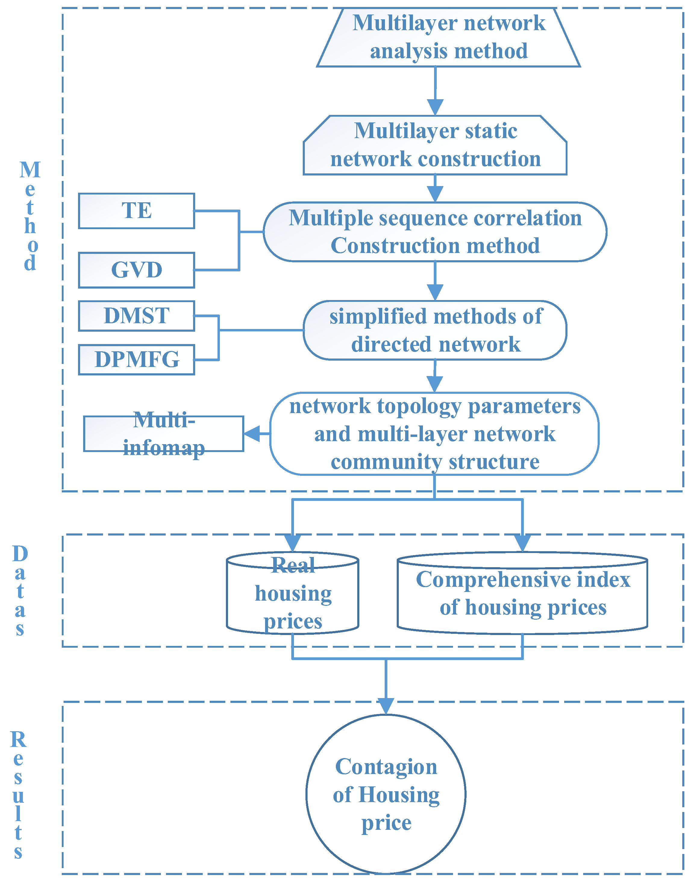
2. Methodologies
2.1. Construction of Multilayer Networks
2.1.1. Calculation of Transfer Entropy
2.1.2. Calculation of Generalized Variance Decomposition
2.1.3. Steps of the DMST Method
- Randomly select a node as the root node;
- Travel all edges and find the smallest entry edges of all points except for the root node. Then, sum up the weighted values of edges to form the new graph. Determine the final minimum arborescence if no cycles exist in the new graph;
- If a ring exists in the new graph, shrink the ring to a point and change the edge weight. The procedure to change edge weights is as follows:
- (1)
- Choose a node () in the ring and set the incoming edge of this node as and outgoing edge as . and refer to the source node and weight, respectively;
- (2)
- Set the new edge weight of node as ;
- (1)
- Return to Step 2 if the new weight graph contains rings;
- Expand the new graph if rings do not exist by the loop-breaking method (Hemminger, 1966; Gabow et al., 1986) [23,24]. The steps of the loop-breaking method are as follows:
- (1)
- Find a loop in the graph;
- (2)
- Remove the edge with the highest weight among the loops, but keep the graph connected;
- (3)
- Repeat this process until there are no loops in the graph (but they are still connected) and obtain the minimum spanning tree.
2.1.4. Steps of the DPMFG Method
- (1)
- By summing symmetric elements, convert the directed network into an undirected network;
- (2)
- Use the undirected PMFG to simplify a fully connected network to a network with only 3 (N − 2) edges remaining;
- (3)
- Restore each edge in the simplified undirected PMFG network to two directed edges, and keep the direction and weight of the side with the highest weight value as the edge and weight of the directed PMFG. Thus, the network is simplified to a directed PMFG network.
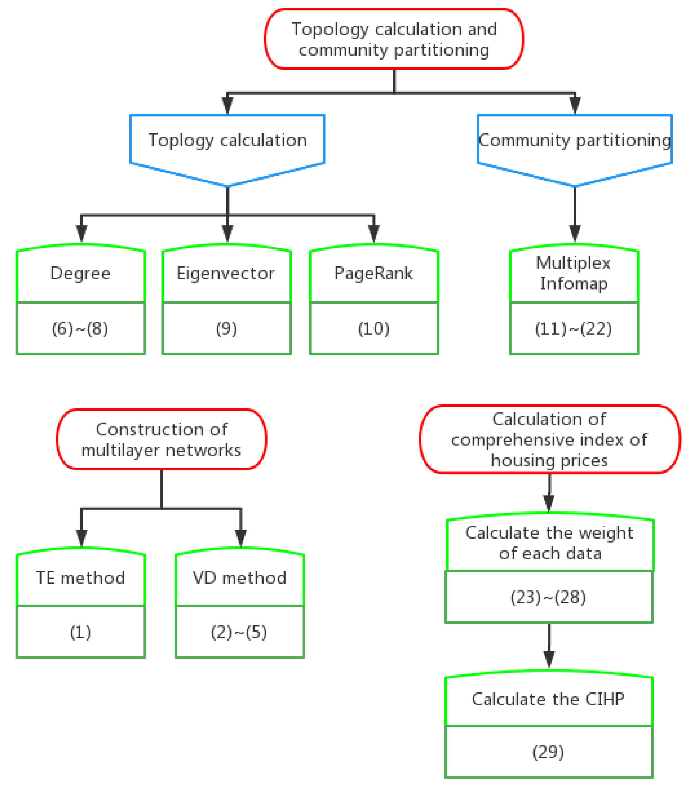
2.2. Topology Calculation and Community Partitioning Method for Multilayer Networks
2.2.1. Centrality in Multilayer Networks
- (1)
- Degree Centrality
- (2)
- Eigenvector Centrality
- (3)
- PageRank Centrality
2.2.2. Multiplex Infomap
2.3. Flowchart of the Methodologies
3. Data and Indicator Processing
3.1. Calculation of Comprehensive Index of Housing Prices
- (1)
- Because the order of magnitude of the indicators may differ, the data must be standardized before calculating the entropy value of each indicator. The indicators selected herein are all positive; therefore, the standardization formula for each indicator is:where is the maximum value of indicator , and is the minimum value of indicator ;
- (2)
- To avoid 0 and negative values when calculating entropy, it is necessary to and add 0.1 to all values.
- (3)
- Determine the proportion of the th index of each city in each year:
- (4)
- Calculate the information entropy of the th index. The lower the entropy value, the greater the difference between the indices. The information entropy is expressed as follows:where .
- (5)
- Calculate the difference coefficient of the th index:
- (6)
- Calculate the weight of th index:
- (7)
- Calculate the comprehensive index of housing price (). Because there is a minimal difference in the dimension of the sales price index between new commercial houses and the secondhand houses, the original data can be used to calculate the CIHP:where denotes the CIHP of city in the th year.
3.2. Analysis of the Comprehensive Index of Housing Prices
3.3. Selection and Source of Real Housing Price Data
4. Results and Analysis
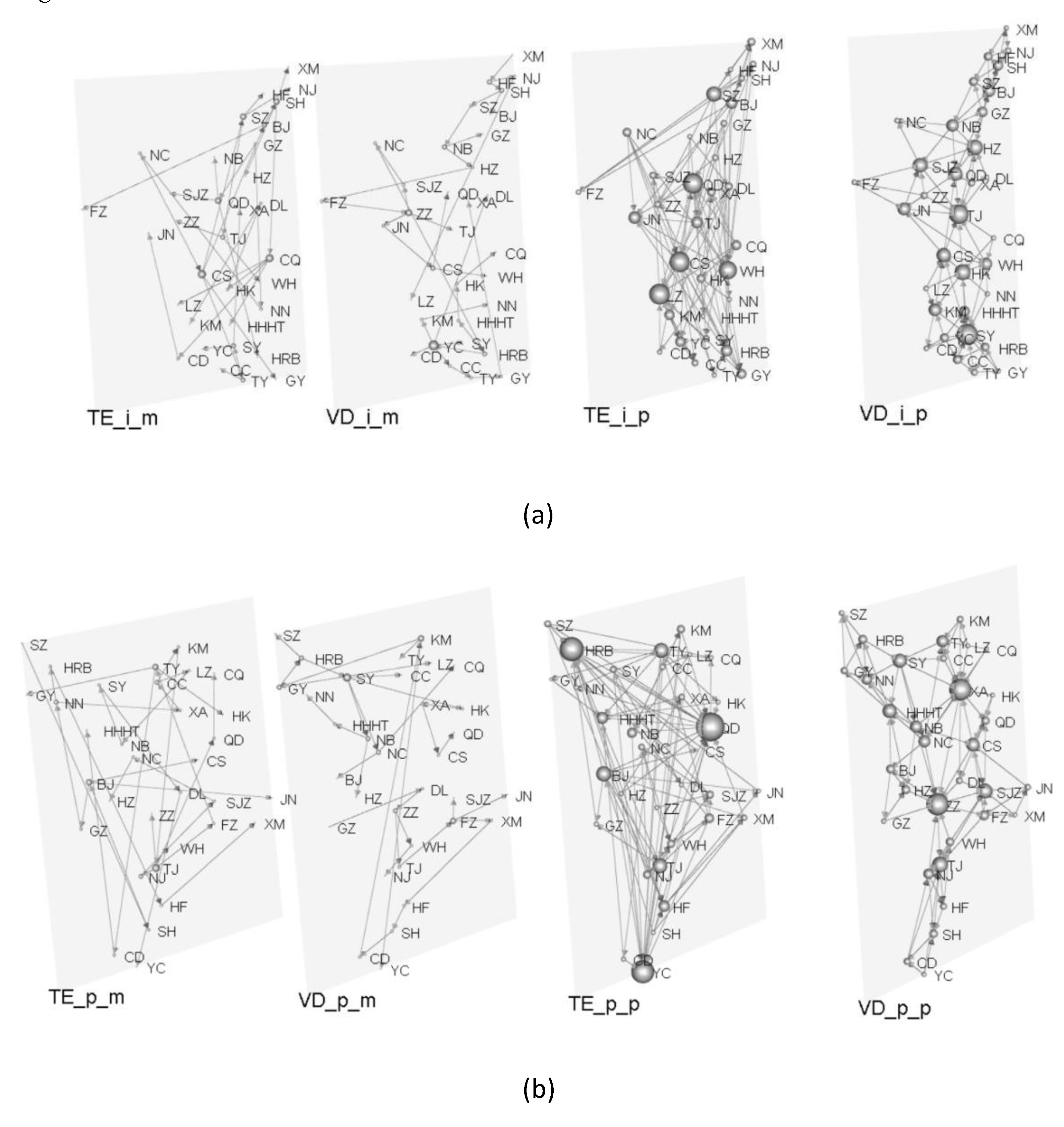
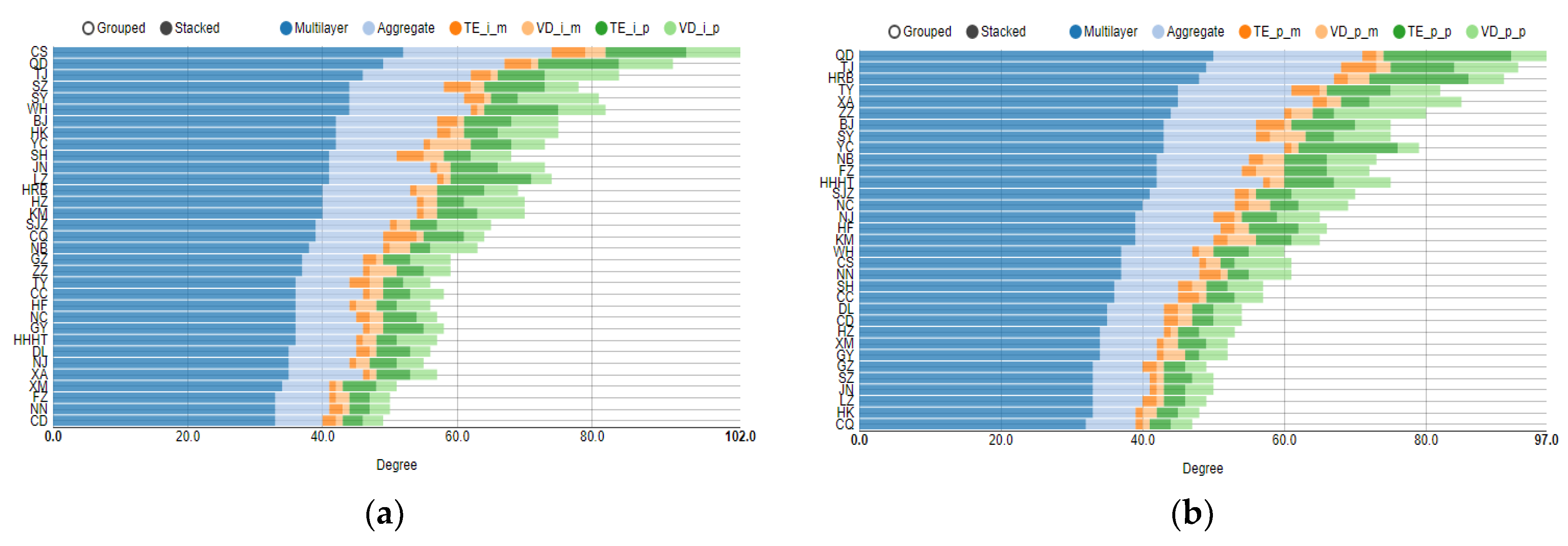
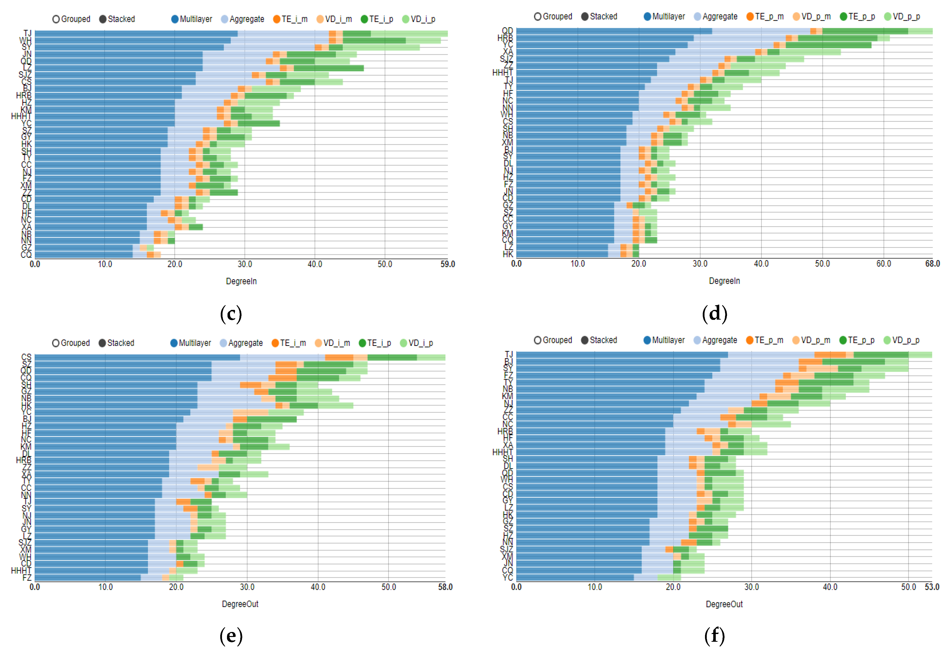
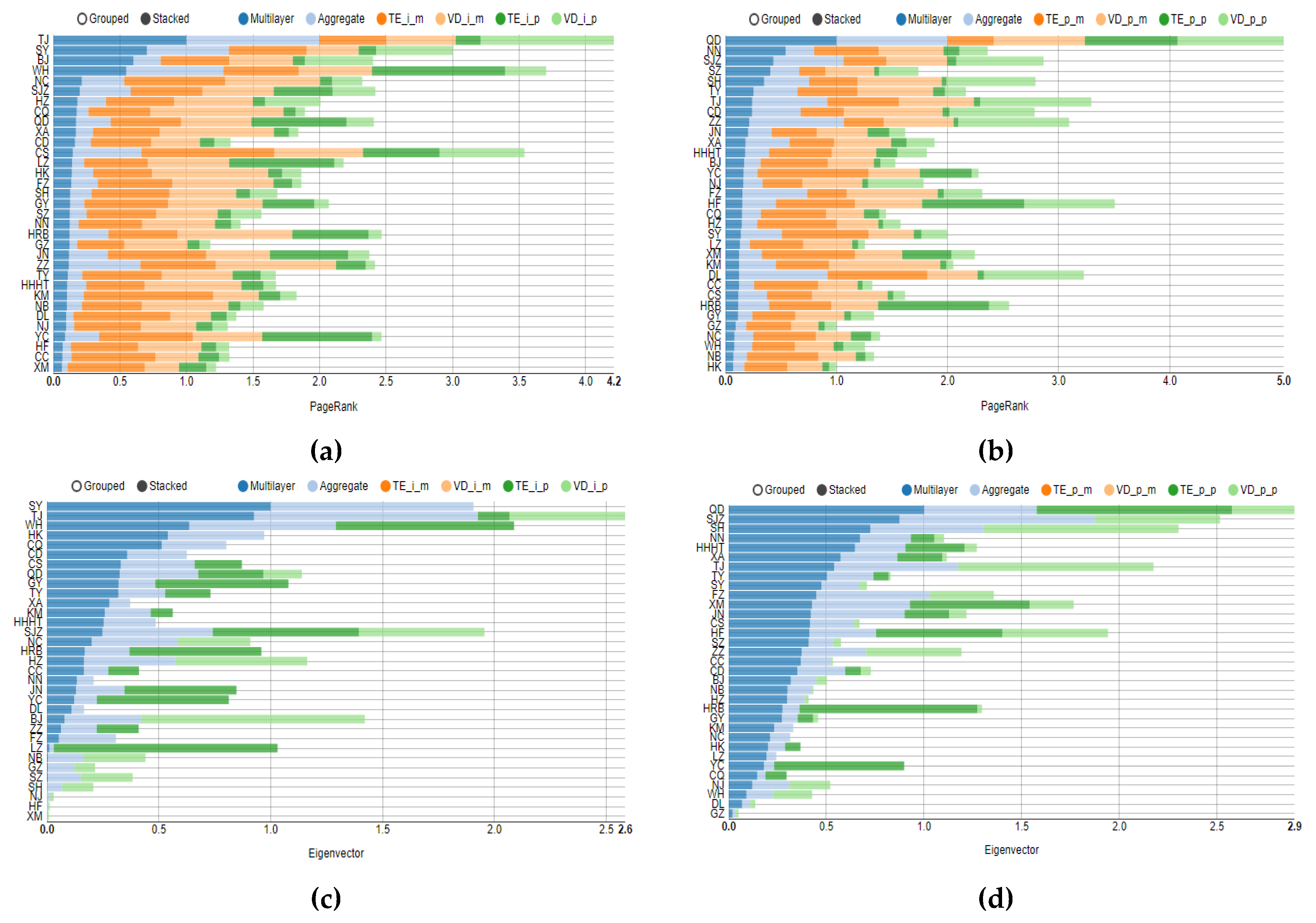
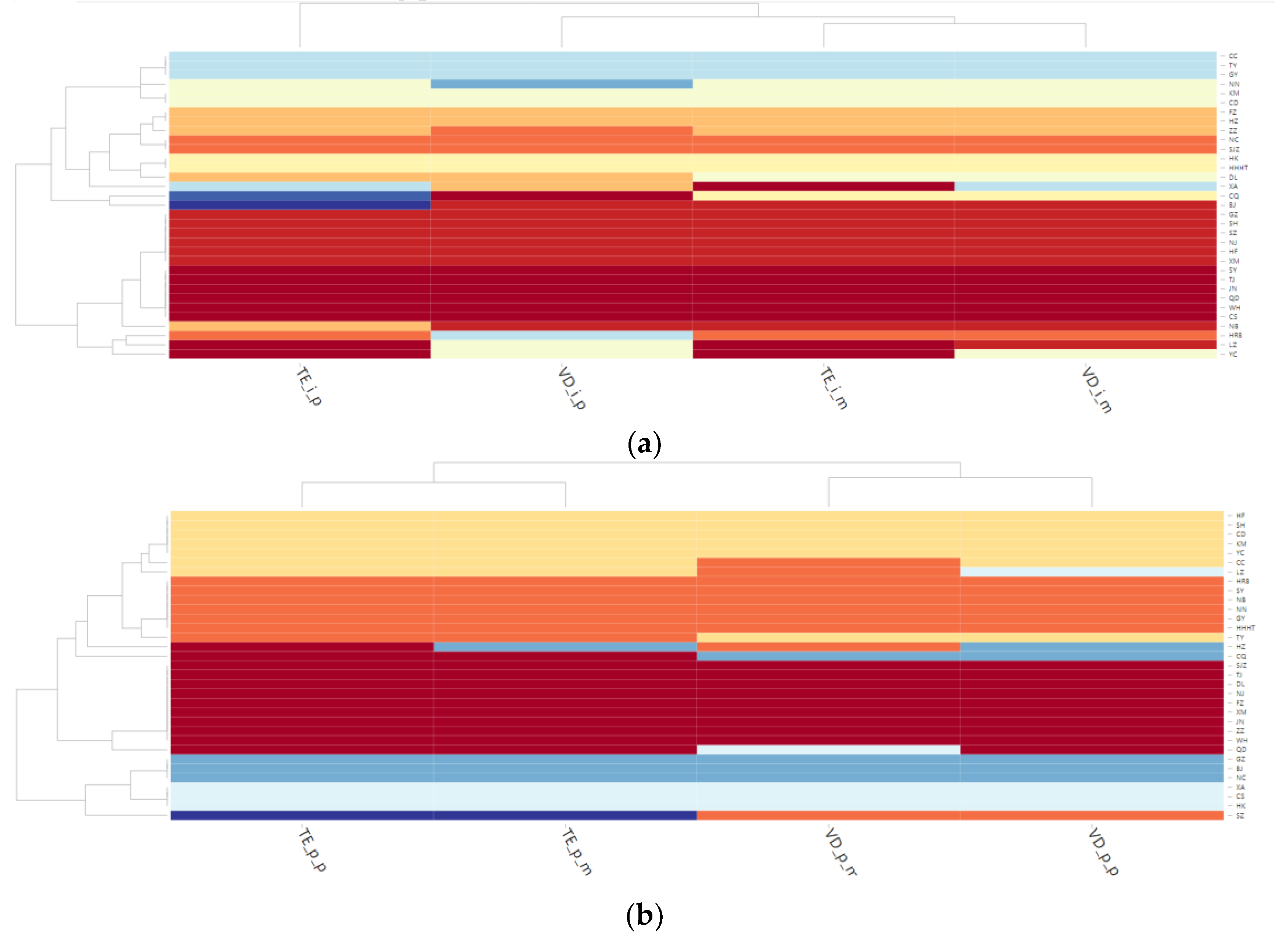
4.1. Topology Analysis of Each Layer in Multilayer Complex Networks
4.2. Multilayer Network Centrality Index Analysis
4.3. Community Analysis of Multilayer Networks
5. Conclusions and Discussion
Supplementary Materials
Author Contributions
Funding
Data Availability Statement
Conflicts of Interest
References
- Li, Z.; Wang, X.J.; Liu, Q. Housing Price Volatility Spillovers in China: From the Perspective of Risk Network. J. Cent. Univ. Financ. Econ. 2021, 4, 114–128. [Google Scholar] [CrossRef]
- Ding, R.X.; Ni, P.F. Regional Spatial Linkage and Spillover Effect of House Prices of China’s Cities—Baced on the Panel Data of 285 Cities from 2005 to 2012. Financ. Trade Econ. 2015, 36, 136–150. [Google Scholar] [CrossRef]
- Chen, L.N.; Wang, H. Empirical Investigation on the Regional Interactions of Real Estate Prices in China. Stat. Res. 2012, 29, 37–43. [Google Scholar] [CrossRef]
- Gong, Y.L.; Haan, J.; Boelhouwer, P. Cross-city spillovers in Chinese housing markets: From a city network perspective. Pap. Reg. Sci. 2020, 99, 1065–1085. [Google Scholar] [CrossRef]
- MacDonald, R.; Taylor, M.P. Regional House Prices in Britain: Long-Run Relationships and Short-Run Dynamics. Scott. J. Political Econ. 1993, 40, 43–55. [Google Scholar] [CrossRef]
- Alexander, C. Seasonality and Cointegration of Regional House Prices in the UK. Urban Stud. 1994, 31, 1667–1689. [Google Scholar] [CrossRef]
- Wang, J.Y.; Liu, X.L. Residential Fundamental Value, Bubble Component and Regional Spillover Effect. China Econ. Q. 2014, 13, 1283–1302. [Google Scholar] [CrossRef]
- Yang, J.; Yu, Z.L.; Deng, Y.H. Housing price spillovers in China: A high-dimensional generalized VAR approach. Reg. Sci. Urban Econ. 2017, 68, 98–114. [Google Scholar] [CrossRef]
- Lv, L.; Liu, H.Y. Research on the Measurement, Network Structure and Influencing Factors of the Spillover Effect of Urban Housing Prices. Econ. Rev. 2019, 2, 125–139. [Google Scholar] [CrossRef]
- Li, Z.; Liu, Q.; Liang, Q. A Study on Forestalling China’s Systemic Risk Based on Financial Industry and Real Economy Interacted Network. Stat. Res. 2019, 36, 23–37. [Google Scholar] [CrossRef]
- Liu, X.L.; Gu, S.T. Research on risk spillovers from the real estate department to financial system based on AR-GARCH-CoVaR. Syst. Eng. Theory Pract. 2014, 34, 106–111. [Google Scholar]
- Liu, H.H.; Chen, S.H. Nonlinear relationships and volatility spillovers among house prices, interest rates and stock market prices. Int. J. Strateg. Prop. Manag. 2016, 20, 371–383. [Google Scholar] [CrossRef]
- Yamaka, W.; Liu, J.X.; Li, M.Y.; Maneejuk, P.; Dinh, H.Q. Analyzing the Causality and Dependence between Exchange Rate and Real Estate Prices in Boom-and-Bust Markets: Quantile Causality and DCC Copula GARCH Approaches. Axioms 2022, 11, 113. [Google Scholar] [CrossRef]
- Zeng, X.W.; Liu, Z.D.; Liu, W.Y. Study on Transmission and Volatility Spillover of Housing Prices in China’s Urban Agglomerations. Manag. Rev. 2015, 27, 3–13. [Google Scholar] [CrossRef]
- Chen, M.H.; Liu, H.J.; Sun, Y.N.; He, L.W. Empirical Study on the Characteristics of Network Structure and Its Influence Factors of Urban Housing Price Linkage: Based on Monthly Data of 69 Large and Medium Cities in China. South China J. Econ. 2016, 1, 71–88. [Google Scholar] [CrossRef]
- Chen, M.H.; Wang, S.; Liu, W.F.; Liu, Y.X. Measurement and Analysis of Correlation Effect of Urban Housing Price under the Nonlinear Perspective. China Soft Sci. 2020, 10, 96–106. [Google Scholar]
- Schreiber, T. Measuring information transfer. Phys. Rev. Lett. 2000, 85, 461–464. [Google Scholar] [CrossRef]
- Chen, Y.C. Market Efficiency and Information Flow between Stocks with Different Systematic Risk Based on the Transfer Entropy; Beijing Jiaotong University: Beijing, China, 2014. [Google Scholar]
- Diebold, F.X.; Yilmaz, K. On the network topology of variance decompositions: Measuring the connectedness of financial firms. J. Econom. 2014, 182, 119–134. [Google Scholar] [CrossRef]
- Kwon, O.; Yang, J.S. Information flow between stock indices. EPL Europhys. Lett. 2008, 82, 68003. [Google Scholar] [CrossRef]
- Qiu, L.; Nan, W.Y. Brain Network Constancy and Participant Recognition: An Integrated Approach to Big Data and Complex Network Analysis. Front. Psychol. 2020, 11, 1003. [Google Scholar] [CrossRef]
- Ye, L.; Wang, Y.Z.; Chen, Y.Y. Study on the Risk Spillover Effect between Chinese Financial Institution. J. Stat. Inf. 2019, 34, 54–63. [Google Scholar]
- Hemminger, R.L. On the group of a directed graph. Can. J. Math. 1966, 18, 211–220. [Google Scholar] [CrossRef]
- Gabow, H.N.; Galil, Z.; Spencer, T.H.; Tarjan, R.E. Efficient algorithms for finding minimum spanning trees in undirected and directed graphs. Combinatorica 1986, 6, 109–122. [Google Scholar] [CrossRef]
- De Domenico, M.; Solé-Ribalta, A.; Cozzo, E.; Kivelä, M.; Moreno, Y.; Porter, M.A.; Gómez, S. Mathematical Formulation of Multilayer Networks. Phys. Rev. X 2013, 3, 041022. [Google Scholar] [CrossRef]
- De Domenico, M.; Solé-Ribalta, A.; Omodei, E.; Gómez, S.; Arenas, A. Ranking in interconnected multilayer networks reveals versatile nodes. Nat. Commun. 2015, 6, 6868. [Google Scholar] [CrossRef]
- De Domenico, M.; Lancichinetti, A.; Arenas, A.; Rosvall, M. Identifying Modular Flows on Multilayer Networks Reveals Highly Overlapping Organization in Interconnected Systems. Phys. Rev. X 2015, 5, 011027. [Google Scholar] [CrossRef]
- Daniel, E.; Ludvig, B.; Martin, R. Mapping Higher-Order Network Flows in Memory and Multilayer Networks with Infomap. Algorithms 2017, 10, 112. [Google Scholar]
- Zhang, X.Y. Chinese Commercial Banks: Balance Development and Secruity. J. Quant. Technol. Econ. 2021, 38, 66–87. [Google Scholar] [CrossRef]
- Boccaletti, S.; Bianconi, G.; Criado, R.; Del Genio, C.I.; Gómez Gardeñes, J.; Romance, M.; Sendiña Nadal, I.; Wang, Z.; Zanin, M. The structure and dynamics of multilayer networks. Phys. Rep. 2014, 544, 121–122. [Google Scholar] [CrossRef] [Green Version]


| Description | Formula Number | References |
|---|---|---|
| 2.1 Construction of multilayer networks | ||
| Network constructed by TE method | (1) | Schreiber (2000) [17], Chen et al. (2014) [18] |
| Network constructed by VD method | (2)~(5) | Diebold and Yilmaz (2014) [19] |
| 2.2 Topology calculation and community partitioning method for multilayer networks | ||
| Degree centrality | (6)~(8) | Domenico et al. (2013) [25], Domenico et al. (2015) [26] |
| Eigenvector centrality | (9) | |
| PageRank centrality | (10) | |
| Multiplex Infomap | (11)~(22) | Domenico et al. (2015) [27], Daniel Edler et al. (2017) [28], |
| 3.1 Calculation of housing price linkage index | ||
| Calculate the weight of each data point | (23)~(28) | Chen Minghua et al. (2020) [16], Zhang Xiaoyan (2021) [29] |
| Calculate the comprehensive index of housing price | (29) | |
| Ranking | City | Abbreviation | CIHP |
|---|---|---|---|
| 1 | Shenzhen | SZ | 110.6588 |
| 2 | Guangzhou | GZ | 107.6885 |
| 3 | Beijing | BJ | 107.54 |
| 4 | Shanghai | SH | 107.1897 |
| 5 | Heifei | HF | 106.8774 |
| 6 | Xiamen | XM | 106.8587 |
| 7 | Nanjing | NJ | 106.3807 |
| 8 | Wuhan | WH | 105.8394 |
| 9 | Nanning | NN | 104.798 |
| 10 | Changsha | CS | 104.6763 |
| 11 | Xi’an | XA | 104.6693 |
| 12 | Kunming | KM | 104.5756 |
| 13 | Zhengzhou | ZZ | 104.5389 |
| 14 | Fuzhou | FZ | 104.5032 |
| 15 | Shenyang | SY | 104.4324 |
| 16 | Hangzhou | HZ | 104.3276 |
| 17 | Huhehaote | HHHT | 104.1595 |
| 18 | Shijiazhuang | SJZ | 103.9711 |
| 19 | Yinchuan | YC | 103.8835 |
| 20 | Chongqing | CQ | 103.8156 |
| 21 | Guiyang | GY | 103.7865 |
| 22 | Tianjin | TJ | 103.7282 |
| 23 | Nanchang | NC | 103.7266 |
| 24 | Haerbin | HRB | 103.6739 |
| 25 | Dalian | DL | 103.6114 |
| 26 | Ningbo | NB | 103.4872 |
| 27 | Taiyuan | TY | 103.4435 |
| 28 | Chengdu | CD | 103.4259 |
| 29 | Jinan | JN | 103.4219 |
| 30 | Changchun | CC | 103.2341 |
| 31 | Lanzhou | LZ | 102.9835 |
| 32 | Qingdao | QD | 102.8244 |
| 33 | Haikou | HK | 102.3365 |
| City | PageRank | Eigenvector | Degree | Degree-In | Degree-Out | Rank in Top 10 | |||||
|---|---|---|---|---|---|---|---|---|---|---|---|
| CIHP | Price | CIHP | Price | CIHP | Price | CIHP | Price | CIHP | Price | ||
| TJ | 1 | 7 | 2 | 7 | 3 | 2 | 1 | 8 | 22 | 1 | 9 |
| QD | 9 | 1 | 8 | 1 | 2 | 1 | 4 | 1 | 2 | 16 | 9 |
| SY | 2 | 20 | 1 | 9 | 4 | 7 | 3 | 18 | 22 | 2 | 7 |
| BJ | 3 | 13 | 23 | 19 | 7 | 7 | 9 | 18 | 10 | 2 | 6 |
| TY | 24 | 6 | 10 | 8 | 21 | 4 | 18 | 9 | 19 | 5 | 6 |
| SJZ | 6 | 3 | 14 | 2 | 16 | 13 | 7 | 5 | 28 | 29 | 5 |
| WH | 4 | 31 | 3 | 31 | 4 | 18 | 2 | 13 | 28 | 16 | 4 |
| XA | 10 | 11 | 11 | 6 | 27 | 4 | 26 | 4 | 15 | 12 | 4 |
| CS | 12 | 26 | 7 | 13 | 1 | 18 | 7 | 13 | 1 | 16 | 4 |
| SH | 16 | 5 | 30 | 3 | 10 | 21 | 18 | 15 | 5 | 16 | 4 |
| ZZ | 23 | 9 | 24 | 16 | 19 | 6 | 18 | 6 | 15 | 9 | 4 |
| YC | 30 | 14 | 21 | 28 | 7 | 7 | 11 | 3 | 9 | 33 | 4 |
| NC | 5 | 30 | 15 | 25 | 21 | 14 | 26 | 10 | 11 | 10 | 3 |
| CQ | 8 | 18 | 5 | 29 | 16 | 33 | 32 | 26 | 2 | 29 | 3 |
| HK | 14 | 33 | 4 | 26 | 7 | 28 | 15 | 32 | 5 | 16 | 3 |
| FZ | 15 | 16 | 25 | 10 | 31 | 10 | 18 | 18 | 33 | 4 | 3 |
| SZ | 18 | 4 | 29 | 15 | 4 | 28 | 15 | 26 | 2 | 22 | 3 |
| NN | 19 | 2 | 19 | 4 | 31 | 18 | 30 | 10 | 19 | 22 | 3 |
| HRB | 20 | 27 | 16 | 22 | 13 | 3 | 9 | 2 | 15 | 12 | 3 |
| JN | 22 | 10 | 20 | 12 | 10 | 28 | 4 | 18 | 22 | 29 | 3 |
| HHHT | 25 | 12 | 13 | 5 | 21 | 10 | 11 | 6 | 28 | 12 | 3 |
| NB | 27 | 32 | 27 | 20 | 18 | 10 | 30 | 15 | 5 | 5 | 3 |
| CD | 11 | 8 | 6 | 18 | 31 | 23 | 25 | 18 | 28 | 16 | 2 |
| LZ | 13 | 21 | 26 | 27 | 10 | 28 | 4 | 32 | 22 | 16 | 2 |
| HZ | 7 | 19 | 17 | 21 | 13 | 25 | 11 | 18 | 11 | 22 | 1 |
| GY | 17 | 28 | 9 | 23 | 21 | 25 | 15 | 26 | 22 | 16 | 1 |
| GZ | 21 | 29 | 28 | 33 | 19 | 28 | 32 | 26 | 5 | 22 | 1 |
| KM | 26 | 23 | 12 | 24 | 13 | 15 | 11 | 26 | 11 | 7 | 1 |
| NJ | 29 | 15 | 31 | 30 | 27 | 15 | 18 | 18 | 22 | 8 | 1 |
| HF | 31 | 17 | 32 | 14 | 21 | 15 | 26 | 10 | 11 | 12 | 1 |
| DL | 28 | 24 | 22 | 32 | 27 | 23 | 26 | 18 | 15 | 16 | 0 |
| CC | 32 | 25 | 18 | 17 | 21 | 21 | 18 | 26 | 19 | 10 | 0 |
| XM | 33 | 22 | 33 | 11 | 30 | 25 | 18 | 15 | 28 | 29 | 0 |
Publisher’s Note: MDPI stays neutral with regard to jurisdictional claims in published maps and institutional affiliations. |
© 2022 by the authors. Licensee MDPI, Basel, Switzerland. This article is an open access article distributed under the terms and conditions of the Creative Commons Attribution (CC BY) license (https://creativecommons.org/licenses/by/4.0/).
Share and Cite
Qiu, L.; Su, R.; Wang, Z. Research on China’s Risk of Housing Price Contagion Based on Multilayer Networks. Entropy 2022, 24, 1305. https://doi.org/10.3390/e24091305
Qiu L, Su R, Wang Z. Research on China’s Risk of Housing Price Contagion Based on Multilayer Networks. Entropy. 2022; 24(9):1305. https://doi.org/10.3390/e24091305
Chicago/Turabian StyleQiu, Lu, Rongpei Su, and Zhouwei Wang. 2022. "Research on China’s Risk of Housing Price Contagion Based on Multilayer Networks" Entropy 24, no. 9: 1305. https://doi.org/10.3390/e24091305