Article

Numerical Modeling and Experimental Validation of Heat Transfer Characteristics in Small PTCs with Nonevacuated Receivers

Solar Thermal Testing Laboratory, ENEA Research Centre Trisaia, I-75026 Rotondella, MT, Italy
*
Author to whom correspondence should be addressed.
Solar 2023, 3(4), 544-565; https://doi.org/10.3390/solar3040030
Submission received: 30 June 2023 / Revised: 6 September 2023 / Accepted: 7 October 2023 / Published: 12 October 2023
(This article belongs to the Special Issue Recent Advances in Solar Thermal Energy)

Abstract

:
The development of small-sized parabolic trough collectors (PTCs) for processing heat production at medium temperatures (100–250 °C) represents an interesting approach to increase the utilization of solar thermal technologies in industrial applications. Thus, the development of simplified models to analyze and predict their performance under different operative and climatic conditions is crucial for evaluating the application potential of this low-cost technology. In this paper, we present a numerical method that by combining three-dimensional finite element simulations (implemented with COMSOL Multiphysics software version 6.1) with a one-dimensional analysis (based on a MATLAB script) allows for the theoretical determination of the power output of a small-PTC with a nonevacuated tubular receiver operating at a medium temperature. The finite element model considers both the nonuniformity of the concentrated solar flux on the receiver tube (evaluated using Monte Carlo ray-tracing analysis) and the establishment of natural convection in the air gap between the glass envelope and absorber tube. The model calculates, for several values of direct normal irradiance (DNI) and inlet temperatures, the thermal power transferred to the heat transfer fluid (HTF) per unit length. The data are fitted using the multiple linear regression method, obtaining a function that is then used in a one-dimensional multi-nodal model to estimate the temperatures and the heat gains along the receiver tube. The outputs of the model are the outlet temperature and the total thermal power transferred to the HTF. In order to validate the developed methodology for the assessment of the heat transfer characteristics in the small-PTC with a nonevacuated receiver, an experiment at the ENEA Trisaia—Solar Thermal Collector Testing Laboratory was carried out. This work compares the theoretical data with those acquired through experimentation, obtaining a good agreement, with maximum differences of 0.2% and 3.6% for the outlet temperatures and the power outputs, respectively.

1. Introduction

To date, the literature on the simulation of parabolic trough collectors (PTCs) is quite extensive [1] and presents a considerable amount of work (for first orientation, see the bibliography in [2]). These works concern both the optical simulation and thermo-fluid dynamics, which are very often combined; in fact, an optical simulation results in the distribution of the radiant flux on the receiver tube, which is the input to the thermo-fluid dynamic simulation. Many of these works also present a comparison between calculated and measured data applied to PTCs available on the market. In particular, in the work conducted in [2,3], three-dimensional (3D) analyses of the receiving tube using, for the optical part, ray-tracing-based software to take into account the nonuniform radiant flux on the receiver were performed. A thermo-fluid dynamic simulation was instead carried out using FLUENT code in [4], which is based on the finite volume method (FVM) [5]. The obtained results were compared to the experimental data, showing differences of at most a few percent. A detailed description of the ray-tracing software developed by the authors and its main features can be found in [6]. In another work [7], a 3D analysis using ray-tracing software combined with FLUENT code was performed. However, this work presents transient calculations, the knowledge of which is of great importance for the structural analysis of the receiver and the identification of the causes of possible breakages due to differential thermal expansions.
In another work using the same FVM code [8], knowing that the use of obstacles in PTCs is an interesting way of improving the collector’s performance but which results in increasing pressure losses, the authors’ aim was to numerically explore the impact of introducing obstacles into the receiver tube of a PTC on the heat transmission and the overall thermal performance. The first part of the work analyzed the effects of geometrical parameters on the fluid motion, heat transfer and performance. The second part investigated the impact of the use of nanoparticles on the temperature profile and heat transfer performance. The FLUENT code was then exploited to create and mesh the geometrical three-dimensional model.
In a similar work [9], a realistic 3D receiver–1D heat transfer fluid (HTF) model, under an unsteady formulation of the partial differential equations, was implemented to properly calculate the receiver’s thermal distribution. The model was solved using the FVM involving the nonuniform heat flux distribution on the receiver tube and a Monte Carlo ray-tracing (MCRT) method implemented in SolTrace. Its main novelty is the introduction of a correction factor in the standard heat transfer coefficient correlations for uniform boundary conditions due to their inability to correctly predict the absorber’s thermal profiles. The model was validated using the AZTRAK platform at Sandia National Laboratories. The general model is implemented in Fortran code based on the FVM, whose systems of algebraic equations are solved iteratively until the convergence criterion is met.
In another work [10], also based on the classical combination of the MCRT method for the optical problem and the 3D-FVM for the thermo-fluid dynamic problem, a new efficient model of convective heat transfer in the HTF was created based on Navier–Stokes equations. This study represents the first attempt to mathematically generalize the thermo-fluid analysis in a parabolic trough receiver. Unlike previous studies, the modeling was carried out using a fully dimensionless thermo-fluid mathematical model and a dimensionless numerical algorithm.
In [11], optical and thermo-fluid dynamic analyses are re-proposed, the latter of which is conducted with the FVM in order to discretize the computational domain both in the axial and azimuthal directions. The thermal analysis relative to the fluid inside the absorber is one-dimensional, and the set of algebraic equations, obtained by applying the FVM, is solved by means of a direct solver. The optical model, based on ray-tracing techniques and the FVM, was validated by comparison with analytical data found in the literature, showing good agreement with them. The subsequent validation of the thermal model was carried out comparing the results obtained with the experimental data of the Sandia National Laboratories, also showing, in this case, a good agreement.
In a similar work [12], the authors studied in depth the coupling between single-phase flows of direct steam generation in a PTC with a fast and realistic 3D receiver–1D HTF model, using nonuniform heat flux distribution, which was validated with experimental data from the Direct Steam Solar facility for the heat transfer and absorber thermal field variables.
A one-dimensional thermal analysis based on the finite difference method [13] can be found in [14]. The analyses carried out showed good agreement with the experimental data and with more complex 2D and 3D models. Another analysis using the difference method is reported in [15]; this work describes the mathematical modeling of a PTC in which the HTF had temperature-dependent physical properties for which the authors developed their own mathematical expressions. The mathematical model is governed by three nonlinear partial differential equations of the parabolic type with initial/boundary value conditions. The authors describe a numerical algorithm that combines the finite difference method (based on the semi-implicit predictor–corrector method) with the finite element method (FEM) for the space discretization to obtain an approximate solution for this model. Then, they perform numerical simulations that provide valuable information on the performance and efficiency of a solar PTC plant operating at a specific location.
A different approach to the thermo-fluid dynamic simulation is discussed in [16], in which the balance equations for the heat transfer fluid (HTF), the receiving tube and the glass envelope are written considering a section of the receiving tube with a plane orthogonal to the axis. A system of nonlinear algebraic equations thus obtained was solved using the EES (Engineering Equation Solver) software [17].
A thermo-fluid dynamic analysis based on the FEM [18,19] is carried out in [20]. The model used is 3D and was compared with a 2D analytical model, developed by the German company DLR and implemented using MATLAB code and Sandia Model [21], which is a one-dimensional empirical model whose equations are solved with EES. The results concerning the calculation of losses showed a good agreement between the FEM analysis, Sandia Model and experimental data. Significant differences were instead found in the temperature profiles along the tube.
Finally, two works using a FEM code implemented in COMSOL Multiphysics software are reported. In the first one [22], in order to improve the efficiency and yield of a PTC solar field, the authors undertook such an attempt with the help of the geometric optics and conjugate heat transfer modules in the COMSOL software. The seasonal variabilities of the solar altitude angle and normal intensity of the sun rays are explicitly incorporated to run a step-by-step optimization to determine the rim angle and the effective working hours that maximize the annual heat collection for a given location in India.
In the second one [23], the authors study the possibility of realizing a prototype of PTC that has the main features of highly reduced dimensions, compared to standard PTCs, and modularity. An optical analysis allowed for the selection of the optimal values of the parameters for the parabola, aperture and rim angle. A thermo-fluid dynamics FEM was developed with COMSOL Multiphysics to analyze the relevant physical characteristics and predict the performance of the receiver tube. The efficiency curve of the collector was extracted. Successively, a receiver tube was built based on the indications of the FEM for what concerns the geometry and materials. In order to evaluate the heat loss of the receiver and to validate the FEM analysis, a test bench was realized. The results of the off-sun heat loss tests on the receiver tube are reported for several temperatures. The computational model was in good agreement with the experimental results and, therefore, it has been validated.
The present work consisted of a 3D simulation applied to a small-PTC with a nonevacuated tubular receiver operating at medium temperature (100–250 °C). This type of collector was analyzed and tested (according to the ISO 9806 standard [24]) at the Solar Thermal Testing Laboratory of the ENEA Research Centre Trisaia in Southern Italy.
Most of the works cited in the bibliography refer to high-temperature PTCs with a vacuum gap between the receiver and the glass envelope [25,26]; on the other hand, in other works, the calculations under the condition of vacuum loss are also provided [27,28]. Our work instead applies to nonevacuated receivers and the analyses were carried out using as a turbulence model a derivation of the classical k-ε model, known in the literature as a “low Reynolds k-ε” model [29,30].
The calculations were based on a 3D model that takes into account both the gravity effects in the air gap between the glass envelope and absorber tube and in the fluid inside the receiver and the nonuniformity of the concentrated solar flux on the outer surface of the receiver. In fact, the gravity effects increase as the air pressure increases in the cavity and, as the tube is sealed, the air pressure increases with the operating temperature. This trend was determined by means of a 2D transient model applied to a section of the receiver tube. As the pressure is known from the 2D transient simulation, the calculation may be conducted considering the natural convection induced by the gravity. It should be noted that the natural convection induced into the air gap between cover glass and absorber tube is a phenomenon that tends to increase the thermal losses of the collector. Clearly, this method can be generalized to other types of concentrating collectors provided that the geometry of the corresponding receiver is of cylindrical shape. The developed 2D and 3D models allowed for evaluating the thermal power transferred to the circulating fluid in a small portion of the receiver tube, far away from its ends (so as to neglect the end-loss effects). This approximation allows the number of degrees of freedom to be kept, especially in the 3D case, at values not excessively high, making the analysis possible within an acceptable amount of time. In the analyzed tube section, fully developed boundary conditions related to motion and thermal fields have been imposed.

2. Materials and Methods

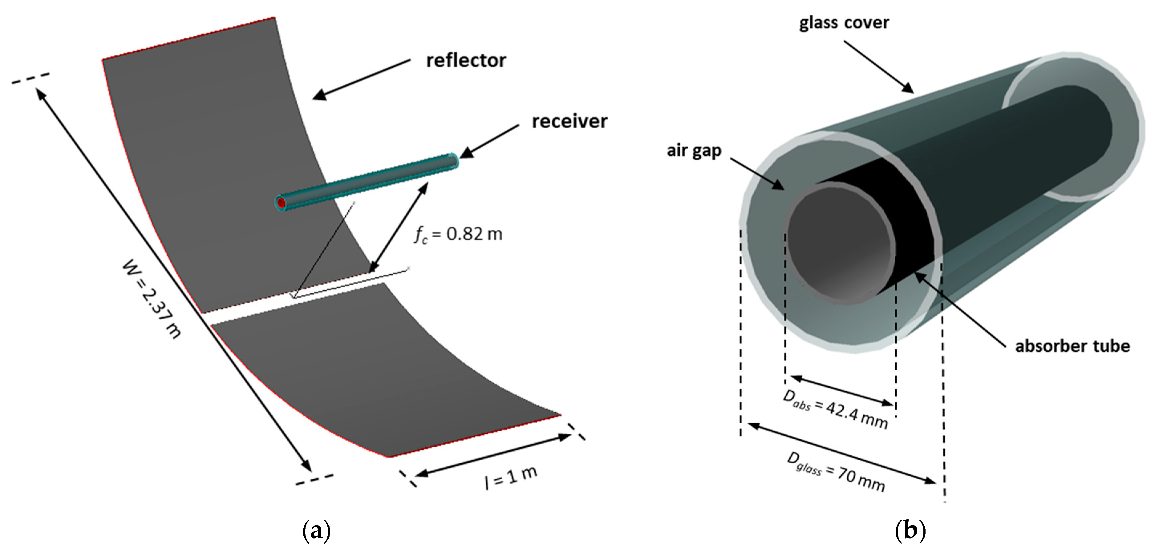
2.1. Description of Collector

The thermo-fluid dynamic models were developed for a small-sized PTC with a nonevacuated tubular receiver. The system is characterized by a primary reflector consisting of a series of linear parabolic mirrors on the bottom of which there is a slit of width corresponding to the receiver tube. The receiver is made up of a stainless-steel absorber pipe, treated with a selective coating, enclosed in a glass tube filled with air at atmospheric pressure. Figure 1 shows both the axonometric view of a portion of the concentrator and the sectional view of the receiver.
Table 1 reports the main geometrical parameters of the small-sized PTC under investigation.

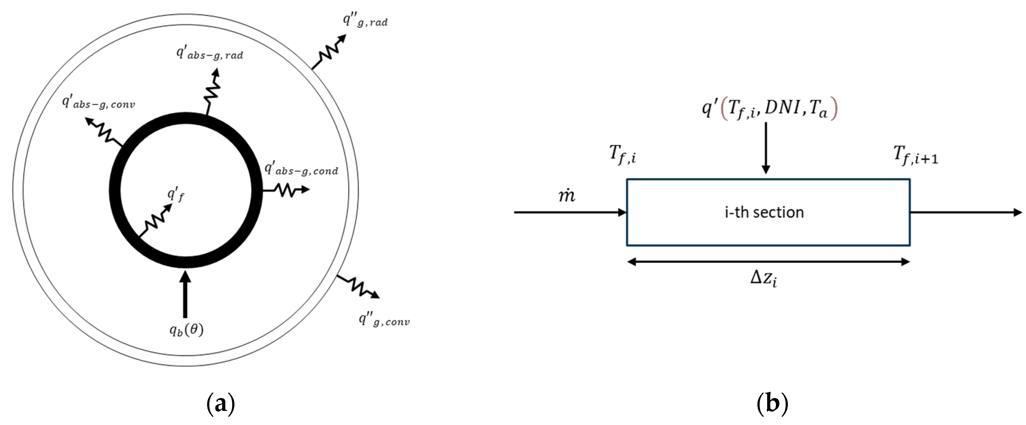
2.2. Heat Transfer in Nonevacuated Parabolic Trough Receiver

In Figure 2 are shown a cross-section of the receiver tube, with inlet and outlet thermal heat flows, and a longitudinal section of a portion of the receiver tube.
The heat transfer in the nonevacuated receiver is characterized by the following steps:
  • Direct normal irradiance (DNI) is concentrated using the parabolic reflecting mirrors. In this study, the slope, specular and tracking errors were considered by introducing an appropriate increase in the angular divergence of the solar beam.
  • The concentrated solar radiation flux is transmitted through the glass envelope and reaches the absorber tube. During this step, a small part of the concentrated solar radiation energy is absorbed by the glass envelope. This amount of energy was considered in the present study.
  • The absorber tube absorbs the concentrated solar flux through the selective coating deposited on the outer surface of the absorber. The angular distribution of the absorbed solar flux was considered in this study.
  • The heat absorbed by the selective coating is conducted to the inner surface of the absorber tube and then transferred to the HTF through convection. At the same time, the selective coating exchanges energy with the inner surface of glass envelope through conduction, convection and radiative exchange in the annular air gap. All these phenomena were considered in this study.
  • The outer surface of the glass envelope dissipates heat towards the environment through convective and radiative exchanges.

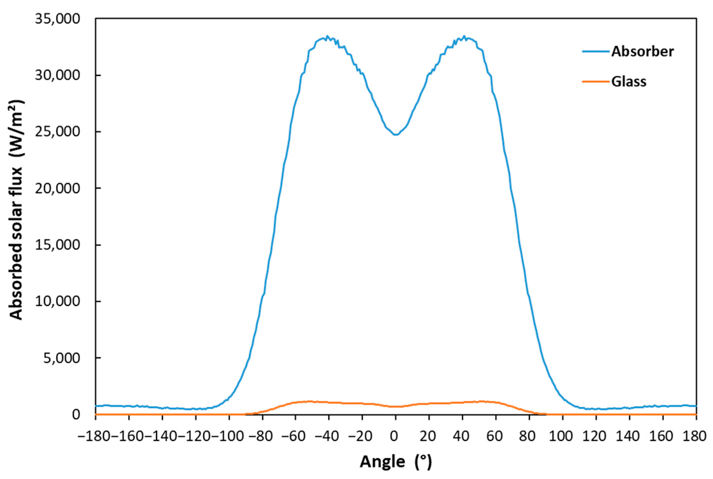
2.3. Concentrated Solar Flux

The ray-tracing TracePro software version 7.4 [31] was used to evaluate the radiant power absorbed by the receiver tube, whose average value on the whole outer surface of the absorber tube is equal to 12.97 kW/m2 for a DNI = 1000 W/m2. Table 2 summarizes the values of the main parameters used for the optical simulation.
Regarding the optical analysis, the following calculation conditions were adopted:
  • Method used: Monte Carlo ray-tracing (MCRT) simulation;
  • Grid pattern: dithered rectangular in which for each cell of the rectangular grid, the starting point of each ray is chosen randomly within the cell with a uniform distribution;
  • Spatial and angular distributions of the solar beam: the rays are distributed uniformly over the grid dimensions, while the direction of each ray is chosen randomly within a Gaussian angular distribution with a half-angle [31] equal to the assigned divergence of solar beam θsb.
For the Gaussian distribution, the half-angle is the angular deviation from the beam axis, where the intensity drops to 1/e2 of the maximum value, and it is twice the standard deviation of the angular distribution [32].
In the statistical ray-tracing method, Gaussian distribution functions of the angular deviations from perfect optics are used to describe all kinds of errors affecting the optical system [33]. The total optical error, including the sun shape error, is then given by the sum of the squares of the individual errors occurring in the system [34]:
  σ t o t 2 = σ s u n 2 + ( 2 σ s l o p e ) 2 + σ m i r r o r 2 + σ t r a c k 2
where σ s u n represents the standard deviation of the sun’s energy distribution, σ s l o p e is the slope error (due to imperfections in the reflecting surface, which cause a doubling of the angular deviation of the reflected rays), σ m i r r o r is the specularity error and σ t r a c k is the tracking error.
Other optical errors, due to imperfections in the manufacture, assembly and operation of the collector, have been omitted in the present study. Therefore, assuming the following main optical errors [33]:
  • Sun shape error σ s u n = 2.6 mrad;
  • Slope error σ s l o p e = 1.9 mrad;
  • Specularity error σ m i r r o r = 2 mrad;
  • Tracking error σ t r a c k = 1 mrad.
We obtained a total optical error equal to σ t o t ≅ 5 mrad, which was used in the MCRT analysis.
Finally, as regard the optical properties of the materials constituting the receiver tube, the analysis took into account:
  • Factory settings of optical parameters;
  • Reflection and refraction of the rays on the glass envelope;
  • Partial reflection of the rays on the absorber surface.
Figure 3 illustrates the angular distribution of the concentrated solar flux absorbed by the receiver tube.

2.4. One-Dimensional Energy Balance Model

In order to carry out the thermal performance of the collector under investigation in different climatic conditions, a one-dimensional model was developed and implemented in MATLAB version 7.13.0 (R2011b) [35]. Starting from the thermal power transferred to HTF per unit length at different operative temperatures and at different levels of solar radiation, the length of the receiver tube was divided into portions of an equal longitudinal dimension to estimate both the trend of the temperature along the tube and the total power absorbed by the HTF. In the following, the methodological approach used [36] is described.
The function characterizing the thermal power transferred to the HTF per unit length, q′ (Tf, DNI, Ta), must satisfy the following differential equation:
m   ˙ c p d T f d z = q T f , D N I , T a
where m   ˙ is the mass flow rate of the diathermic oil, cp is the average specific heat at constant pressure, Tf is the mass-averaged inlet temperature of the HTF, Ta is the ambient temperature, DNI is the direct normal irradiance and z is the axial coordinate of the receiver tube. With reference to Figure 2b, the above equation was applied to a portion of the receiver tube of length Δzi, where with Tf,i and Tf,i+1 mass-averaged inlet and outlet temperatures are indicated, respectively.
Then, the previous differential equation was discretized obtaining the following forward differences equation:
T f , i + 1 = T f , i + q T f , i , D N I ,   T a m ˙   c p T f , i z i
From this equation, knowing the inlet average mass temperature Tf,0 and the expression of the function q′ (Tf,i, DNI, Ta), it was possible to calculate the temperatures in each portion of length Δzi of the receiver tube and, therefore, also the collector outlet’s mass average temperature, Tf,u.
The thermal power transferred to the HTF in each single node, into which the receiver tube was divided, is given by:
Q i ˙ = m ˙   c p T f , i   T f , i T f , i 1
Thus, the total useful power transferred to the circulating fluid is given by:
Q ˙ = i = 1 N Q i ˙
where N is the total number of nodes.

3. Model Equations

The model was implemented, according to the experimental procedure, in stationary turbulent regime. The equations used in the stationary state, applied to fluid (diathermic oil and air gap) and solid domains, are described in the following paragraphs (for the meaning of the symbols, refer to the nomenclature section).

3.1. Equations Applied to the Heat Transfer Fluid Domain

Momentum balance, based on the Reynolds-Averaged Navier–Stokes equations:
ρ u ¯ · 𝛁 u ¯ = 𝛁 · p ¯ I + μ + µ T 𝛁 u ¯ + 𝛁 u ¯ T 2 3 μ + µ T 𝛁 · u ¯ I 2 3 ρ k I + ϱ g
Mass balance:
𝛁 · ρ   u ¯ = 0
Energy balance:
ρ c p u ¯ · 𝛁 T ¯ = 𝛁 · k l + k t 𝛁 T ¯
where k(l) and k(t) are respectively the laminar and turbulent conductivity.
Equations of Low Reynolds k-ε model:
ρ u ¯ · 𝛁 k = 𝛁 · μ + μ T σ k 𝛁 k + P k ρ ϵ
ρ u ¯ · 𝛁 ϵ = 𝛁 · μ + μ T σ c 𝛁 ϵ + C c 1 ϵ k P k C c 2 ρ ϵ 2 k f ε ρ , μ , k ,   ϵ , I w
Equation for the calculation of the wall distance (Eikonal equation):
𝛁 G · 𝛁 G + σ w G 𝛁 · G = 1 + 2 σ w G 4
where the parameters used in the previous equations have the following expressions:
I w = 1 G l r e f 2
μ T = ρ C μ k 2 ϵ f μ   ρ , μ , k ,   ϵ , I w
P k = µ T 𝛁 u ¯   : 𝛁 u ¯ + ( 𝛁 u ¯ T ) 2 3 𝛁 · u ¯ 2 2 3 ϱ k 𝛁 · u ¯
In Equation (6), the natural convection in diathermic oil was considered, although these effects are negligible compared to forced convection. In fact, the quantity Ri = Gr/Re2, known as the Richardson number [37], is much smaller than unity, varying from 7.82 × 10⁻³ to 3.47 × 10⁻² in the temperature range considered.
In Equation (8), related to the balance of thermal energy in a turbulent regime, the turbulent conductivity k(t) appears. It, knowing the Prandtl turbulent number Pr(t) and the turbulent viscosity μ t , is deducible from the following equation [38,39]:
ν t α t = P r t
where ν t = μ t ρ and α t = k t / ρ c p .
For the Pr(t) expression, the following Kays–Crawford correlation was used [38,39].
P r t = 1 P r t + 0.3 P r t c p μ t k 0.3 c p μ t k 2 e k / 0.3 c p μ t P r t 1
where P r t = 0.85.
On the basis of their definitions, k(t) and μ t are not thermophysical properties of the fluid but only of the motion and vary strongly as the position varies.
Regarding Equation (11), it represents a “modified eikonal equation”, which is a mathematical method originally developed for the calculation of the distance of a point from a surface. In our case, it was adapted to calculate the distance from the inner wall of the tube [30].

3.2. Equations Applied to the Air Gap Fluid Domain

The motion in the air gap was assumed to be laminar because the Grashof number [37] varied from 4.01 × 10³ to 1.25 × 10⁴ in the temperature range considered, while the critical value between laminar motion and transition zone was 108. The equations related to laminar motion are the following:
Momentum balance:
ρ u · 𝛁 u = 𝛁 · p I + µ 𝛁 u + 𝛁 u T 2 3 µ 𝛁 · u I + ρ g
Mass balance:
𝛁 · ρ   u = 0
Energy balance:
ρ c p u · 𝛁 T = 𝛁 · k 𝛁 T

3.3. Equations Applied to Solid Domains

For solid domains, represented by the absorber tube and the glass envelope, only the following energy balance equation applies.
𝛁 · k 𝛁 T = 0

3.4. Radiation Heat Transfer

The radiative heat exchange, between the outer surface of the absorber tube and the inner surface of the glass envelope, is evaluated considering both superficies as gray. Each surface is divided into N smaller areas, Ai, the temperatures of which are assumed uniform. The adopted balance equations are the following [40]:
q i = A i ε i 1 ε i σ T i 4 J i
q i = A i ( J i k = 1 N J k F i k )
where qi is the net power lost by surface Ai, ε i is the emissivity of surface Ai and Fik are the view factors between i-th and k-th surface.
Ji is the radiosity that represents the total radiation leaving the surface Ai per unit time and per unit area. Its expression is given by [40]:
J i = ρ i G i + ε i σ T i 4
where Gi is the total radiation incident on surface Ai per unit time and per unit area and ρ i is the reflectance of surface Ai.

3.5. Boundary Conditions

The calculation was carried out on a receiver tube portion of 1 m length far away from the edges, and the boundary conditions used in the simulations are those of fully developed flow.
The values assigned to the main variables used in the boundary conditions are defined as follow:
  • Diathermic oil velocity at the inlet of the receiver [41]:
u z , i n = Γ ρ A β 1 r r t 0.14
where β is given by β = u z , i n u z , i n , m a x = 0.8 ;
  • Turbulence intensity entering the receiver, defined through the following equation [19]:
I T 0 = 2 k 0 3 u z , i n = 0.05
where, given IT0, we can calculate the turbulent kinetic energy k0 at the inlet;
  • Characteristic scale of the turbulence at the inlet, LT0 = 0.07D [30], where D is the inner diameter of the absorber tube;
  • Turbulent kinetic energy dissipation in the input, defined by the following expression depending on k0 and LT0:
ε 0 = C μ 3 4   k 0 3 2 L T 0
  • Gradients of k and ε in the outlet section in the z direction equal to 0, namely:
𝛁 k · n ¯ = 0         𝛁 ε · n ¯ = 0
  • Conductive flux gradients in the z direction, in the outlet and inlet sections, equal to 0;
  • Temperature of the diathermic oil entering the absorber tube, variable from 100 to 250 °C;
  • Concentrated solar flux absorbed by the absorber tube, q b θ , where θ is the angular; coordinate. This flux was deduced from the ray-tracing analysis described in Section 2.3;
  • Absolute pressure in the air gap varying from 1.19 to 1.42 bar depending on the temperature of the diathermic oil entering the receiver tube (as described in Section 3.7);
  • For fluid domains, the inlet flow rates and the outlet pressures are specified;
  • Thermal loss from the glass tube to the ambient air given by the following formula:
q g = q g r a d + q g c o n v = σ   ε g T g 4 T s k y 4 + h w T g T a
where the convective heat flux coefficient is given by h w = 4   v w 0.59   D g 0.42 [2].
From the solution of the model equations with the above boundary conditions, the heat flux per unit length   q z was calculated with the following formula:
q z = 1 l k T n   r t d θ d z
where l is the tube length and the minus sign indicates that q z is directed towards the inner wall of the absorber tube.

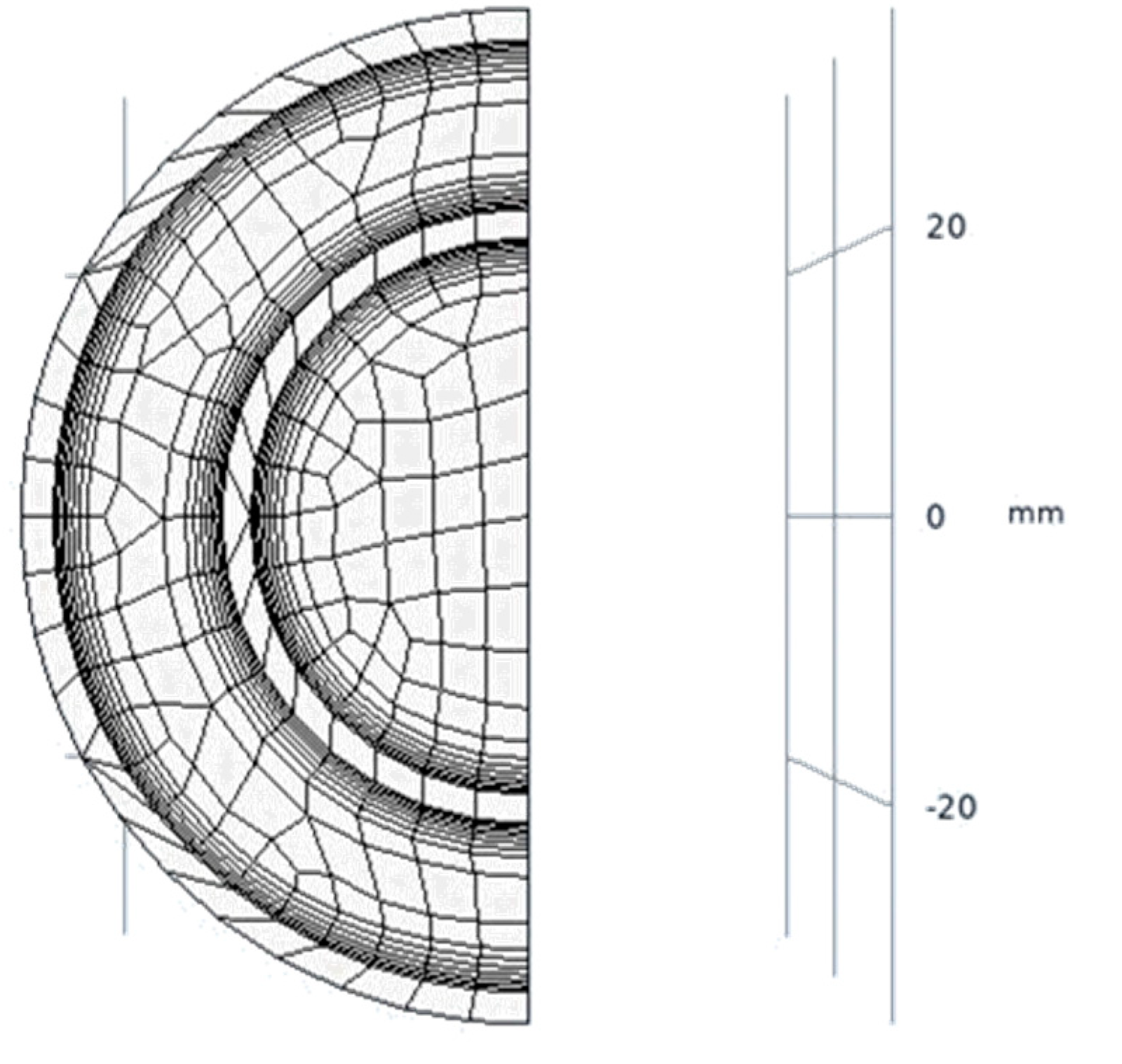
3.6. Mesh and Solver Implemented

The adopted mesh is of the swept type [30] with about 34,000 domain elements per unit length of the receiver tube. The swept mesh allows, in our case, for an accurate solution with a nonexcessive number of elements.
Figure 4 shows the adopted mesh where near each inner wall, separating the fluid and solid domains, the mesh density increased with the introduction of eight layers.
The optimal number of domain elements was determined starting from a coarse mesh and growing until the value of the thermal power per unit length transferred to the diathermic oil differed less than 0.1% between two successive refinements.
Table 3 shows the results obtained from the performed grid sensitivity analysis. These results confirm that the choice of a normal mesh is the most suitable for the present computational problem.
The used convergence criterion is based on a relative tolerance of 0.1% for all fluid dynamic variables considered. The calculation ends when the estimated errors are less than the chosen relative tolerance.
The solver used in the steady-state simulations was based on the “pseudo-time stepping” technique [30] in which the time step is variable and represents the output of a PID controller whose default parameters are calibrated for thermo-fluid dynamics calculations. In transient simulations, the time step adopted is still variable and is calculated so that the estimated error is always lower than the chosen relative tolerance (in our case 0.1%).

3.7. Pressure Variation in the Air Gap

The air gap is closed, and its pressure is a function of the HTF temperature. In order to evaluate this pressure, the transient equations of the system consisting of air, absorber tube and glass envelope were solved using a two-dimensional plane model to have a number of degrees of freedom and a calculation time that were not excessively high. In this model, the diathermic oil is not part of the computational domain and is taken into account by a heat exchange coefficient.
The equations governing the heat transfer of the receiver in the transient regime are shown below. For the air gap domain, the following equations apply:
Momentum balance:
ρ u t + ρ u · 𝛁 u = 𝛁 · p I + µ 𝛁 u + 𝛁 u T 2 3 µ 𝛁 · u I + ρ g
Mass balance:
ρ t + 𝛁 · ρ   u = 0
Energy balance:
c p ρ T t + ρ c p u · 𝛁 T = 𝛁 · k 𝛁 T
For the solid domains, the following energy balance equation applies:
c p ρ T t = 𝛁 · k 𝛁 T
The equations are solved taking into account both the initial conditions of the speed, temperature and pressure in the air gap and the boundary conditions related to the radiant flux incident on the absorber tube and the heat fluxes towards the ambient air and the diathermic oil, which are given by the following formulas:
n ¯ · q = q b θ
q g = q g r a d + q g c o n v = σ   ε g T g 4 T s k y 4 + h w T g T a
q f = h f T s t T f
where the convective coefficient, hf, can be deduced from the following formula:
h f = N u k D
in which the Nusselt number has the following expression [1]:
N u = f 8 R e 1000 P r 1.07 + 12.7 f 8 P r 2 3 1 μ μ w a l l 0.11
f = 0.79 · l n ( R e ) 1.64 2
Once the calculations were carried out, we obtained the trend of the pressures in the air gap at the end of the transient regime, depending on the fluid temperature. The results are summarized in Table 4.

4. Results and Discussion

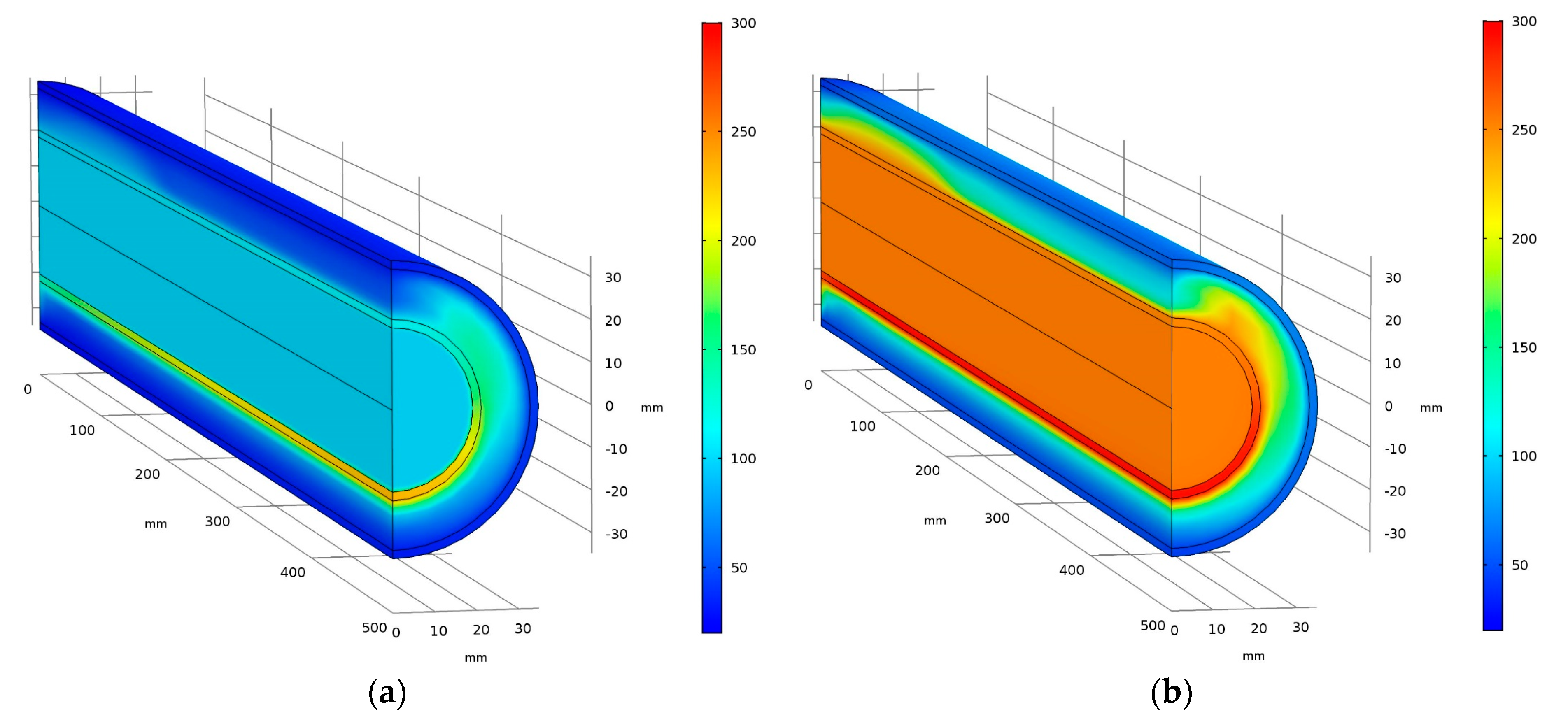
4.1. Three-Dimensional Thermo-Fluid Dynamic Analysis

A three-dimensional thermo-fluid dynamic analysis was carried out using finite element software COMSOL version 6.1 [30]. The implemented model uses the Heat Transfer Module which contains the following main features:
  • Fluid domains are modeled through conjugate heat transfer and nonisothermal flow, which incorporate basic computational fluid dynamic (CFD) equations;
  • Laminar and turbulent flow are both supported and can be modeled with natural and forced convection;
  • Turbulence can be modeled using Reynolds-averaged Navier–Stokes equations trough “k-ε” or “low Reynolds k-ε” models;
  • Pressure work and viscous dissipation can be considered to evaluate the effects on the temperature distribution.
The equations implemented in the developed model are those reported in Section 3, which mostly correspond to the built-in equations integrated in the software. For modeling the radiative exchange between gray surfaces, the equations reported in Section 3.4 were adopted.
Concerning the adopted geometry, a portion of the receiver tube 1 m long was considered, and fully developed flow boundary conditions were used to eliminate the edge effects. The main conditions and values for the parameters used in all simulations are summarized in Table 5.
The calculations were performed varying the inlet fluid temperatures in the range 100–250 °C with steps of 25 °C and considering a DNI variable from 0 to 1000 W/m2 with steps of 250 W/m2.
The COMSOL model was run on the ENEA high-performance parallel computing platform called CRESCO [42], where the typical computational time was approximately 20 min for each 3D simulation.
Table 6 reports the thermal power per unit length transferred to the HTF, obtained from simulations under the abovementioned conditions.
The results at DNI = 0 W/m2 represent the thermal losses of the receiver tube towards the environment and, therefore, are reported with a minus sign.
From the evaluated data matrix, by means of a multilinear least squares regression, q′ (T, DNI, Ta) was determined. It represents the thermal power transferred to the HTF per unit length (W/m) as a function of the average mass temperature of the diathermic oil, the DNI and the ambient temperature. The regression function used was the following:
q T , D N I , T a = a 1 T T a + a 2 T T a 2 + D N I   b 0 + b 1 T T a + b 2 T T a 2
For the definition of the regression model, an approach similar to that used in [43] was adopted. In particular, the thermal power transferred to the HTF per unit length was modeled as the sum of two second-order polynomials, where the first took into account only the thermal losses in the absence of DNI, while the second took into account the effects of the DNI both on the heat gain of the receiver tube and on the overall thermal losses towards the environment.
Table 7 reports the regression parameters obtained from the least squares curve fitting. The table also shows the standard errors related to each fitting parameter and the respective T-ratios whose values, being >> 3 for all estimated parameters, indicate that the parametric identification is statistically significant. The standard errors were evaluated [44] by calculating the covariance matrix C = ( M T ·   M ) 1 , where M is the design matrix of the fitting problem, whose diagonal elements are the variances (squared uncertainties) of the fitting parameters.
The RMSE, obtained from the comparison between the thermal powers transferred to the HTF per unit length predicted by the FEM-CFD model and the thermal powers transferred to the HTF per unit length obtained from the fitted curve, was equal to 1.73 W/m.
Figure 5 reports the thermal fields in the receiver tube for the two extreme temperatures considered in the simulation. These thermal maps point out the flow distortion in the air gap due to the buoyancy forces and the nonuniform distribution of the concentrated solar flux.

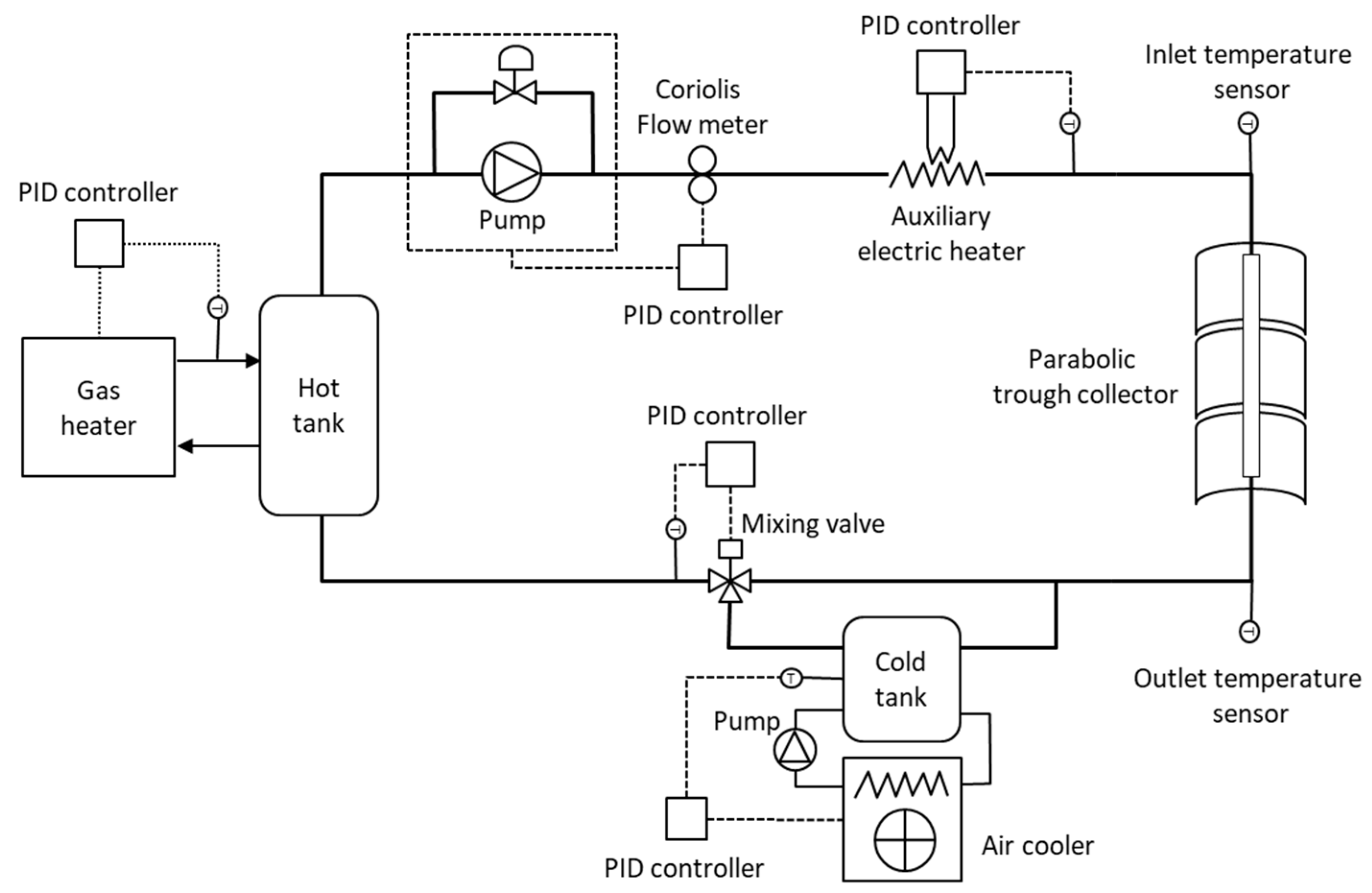
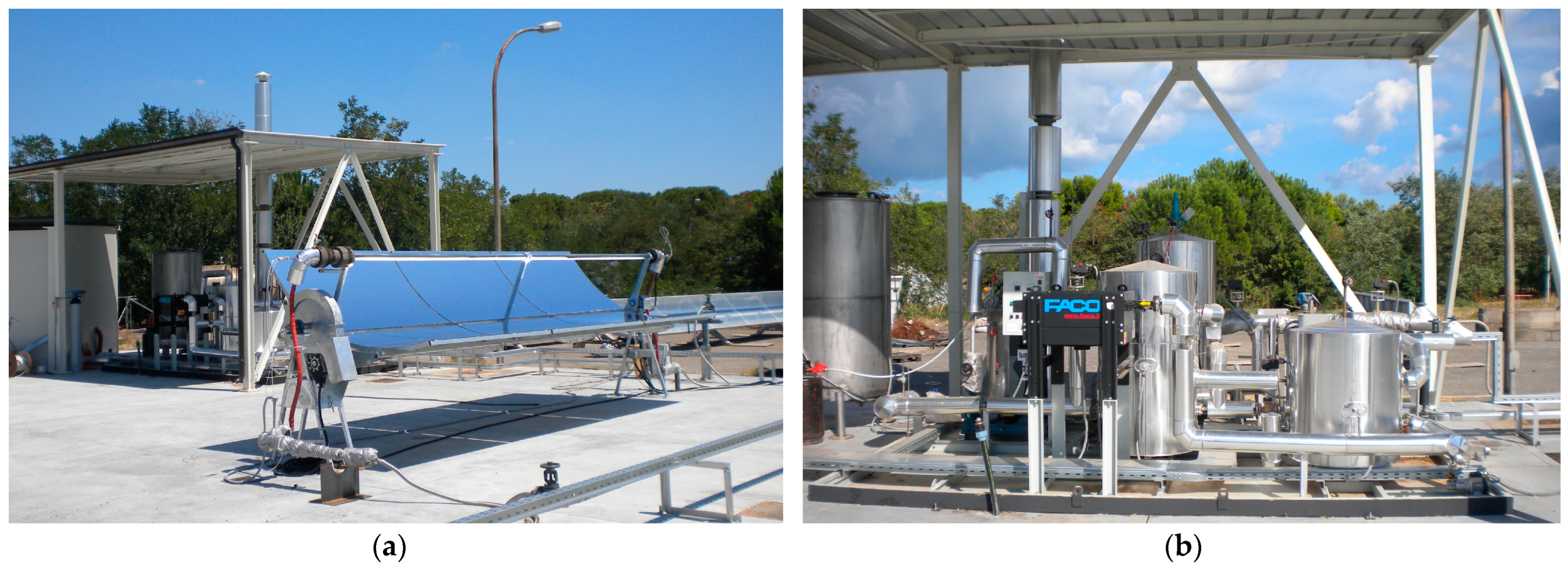
4.2. Experimental Set-Up and Results Obtained

Figure 6 shows a schematic view of the experimental set-up used to evaluate the power output of the parabolic trough collector under investigation. The test rig, consisting of a closed loop that used diathermic oil as the thermal fluid vector, allowed for carrying out, in compliance with the requirements of the ISO 9806 standard [44], the energy performance characterization of concentrating solar collectors in a temperature range between 100 and 250 °C.
A primary heating circuit, consisting of an oil tank heated by a gas burner (thermal power of 50 kW), allowed for setting the working temperature to the desired value. A secondary heating circuit, consisting of an inline auxiliary electric heater (electrical power of 5 kW), allowed for fine-tuning the temperature at the collector inlet to satisfy the stability condition required by the ISO 9806 standard (admissible variation within 0.1 °C). A heat dissipation system, consisting of an additional oil tank cooled by an air heat exchanger, allowed the plant to extract the heat produced by the collector to bring the temperature of the diathermic oil back to the input value. Finally, a flow control system adjusted the flow rate at the test value by means of a pump that recirculated the diathermic oil into a closed loop, from which the desired flow is tapped.
The test facility was equipped with a distributed control system (DCS) for the supervision and control of the process variables, including the temperature entering the small-PTC under test, the process mass flow rate, the temperature leaving the cooling system and the temperatures of the hot and cold tanks. Independent PID regulators were implemented on board the DCS, which allowed for the monitoring and control of each process variable during the test through a user-friendly graphical interface.
A PC-based data acquisition system (DAQ) allowed for the sampling and data logging of all thermo-hydraulic and climatic variables. The DAQ system, based on a National Instruments NI-SCXI 1001 device (equipped with several modules for RTDs, voltages and currents acquisition), performed the analog-to-digital conversion of all signals through real-time sampling. An integrated signal conditioning system supplied the RTD sensors and amplified and filtered the input signals.
A Coriolis effect flowmeter (model Micro-Motion F050) was used to measure the mass flow rate of the diathermic oil with an accuracy less than 0.2%. The inlet and outlet temperatures were monitored by means of 4-wire thermo-resistances Pt 100 class A with an accuracy better than 0.2 K. The DNI was measured with a Class 1 pyrheliometer (model EKO MS-56) mounted on an EKO Instruments sun tracker, with an average instrumental error of ±10 W/m2. Finally, the ambient temperature was measured with a thermo-hygrometer (model VAISALA HMP63), suitably ventilated and shielded from solar radiation, with an accuracy greater than 0.5 K.
The measuring instruments used to acquire the process and climatic variables were calibrated in our laboratory by comparison with reference standards calibrated in accredited metrological institutes. Below are reported the standard uncertainties of each directly measured physical quantity:
  • Temperature: u = 0.08 °C;
  • Flow rate: u = 0.1%;
  • Direct solar irradiance: u = 6 W/m2;
  • Ambient temperature: u = 0.3 °C.
In order to avoid the end-loss effects due to the finite length of the receiver tube, the collector was oriented in east–west direction. All tests were performed in the steady-state, and useful data were acquired only in time periods around the local solar noon, when the DNI was orthogonal to the collector’s aperture area and, consequently, the effects of the incident angle modifier (IAM) are negligible.
The photos in Figure 7 show the experimental set-up with the small-PTC during the operational phase and the details of the test plant, with the main components indicated.
Table 8 summarizes the average test conditions recorded during the field tests carried out on the concentrator object of the theoretical and experimental analysis.
Table 9 reports the experimental data obtained during the field tests, executed in agreement with the requirements of the ISO 9806 standard. All data refer to steady-state values, acquired every 5 s and averaged over a time period of 1 min.
The power extracted from the collector, given by Q m e a s = m ˙ c p , m ( T o u t T i n ) , was determined with a maximum relative standard uncertainty equal to 1.8%, obtained from the propagation of the errors associated with the directly measured data. The specific heat at a constant volume of the diathermic oil was instead determined by means of the following linear correlation c p , m = 3.7134   ( T m + 273.15 ) + 450.39 , deduced from the data reported in the datasheet [45].

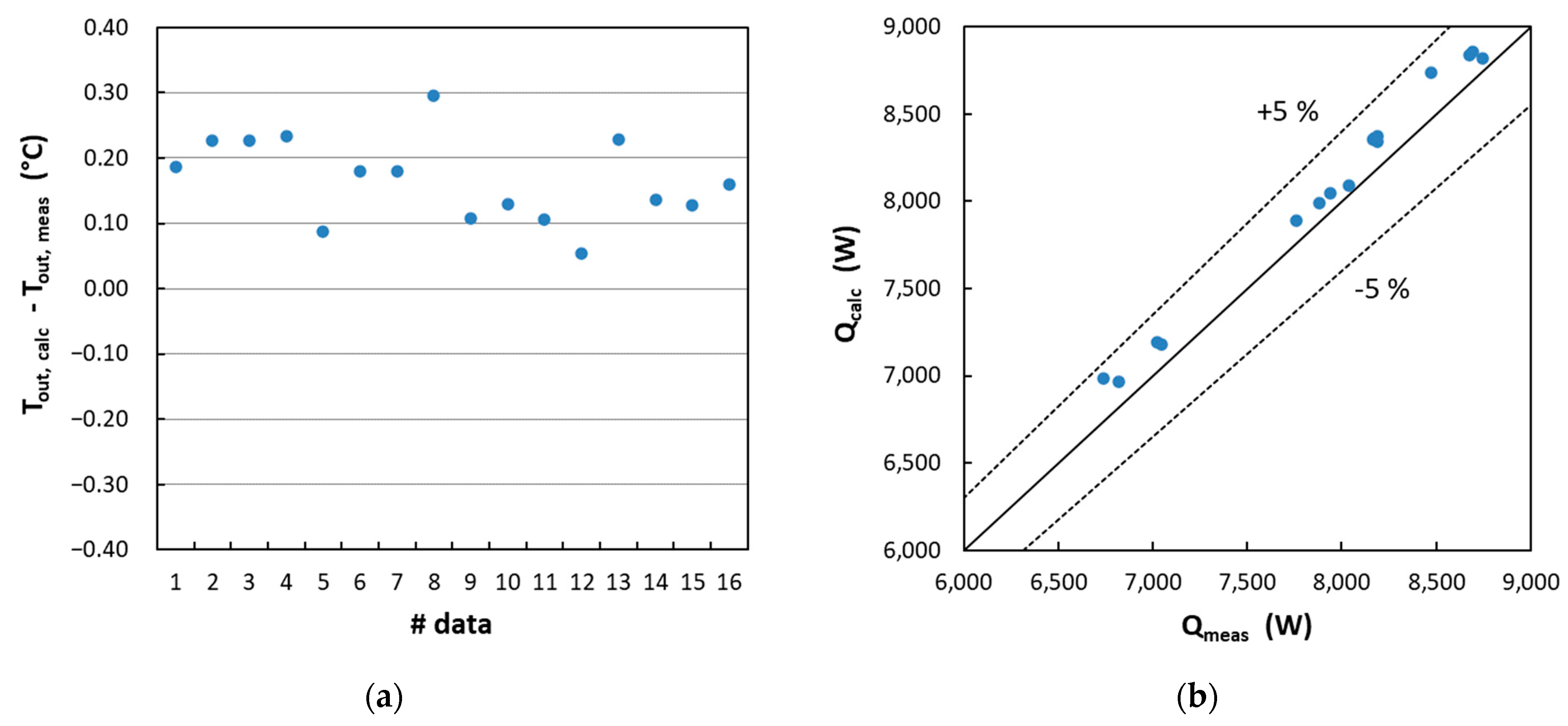
4.3. Comparison between Theoretical and Experimental Data

The calculated values, obtained with the procedure illustrated in Section 2.4, in which the receiver tube was divided into 30 nodes, each 20 cm long, were compared with those obtained experimentally. In Table 10, the percentage differences between the theoretical and measured values are shown.
From the data reported in Table 10, it can be seen that the model slightly overestimated the temperatures and powers. In absolute terms, the maximum difference for the outlet temperatures was around 0.3 °C (corresponding to a maximum percentage difference of 0.2%), while for the thermal powers transferred to HTF, the maximum difference was approximately 263 W (corresponding to a maximum percentage difference of 3.6%).
Figure 8 shows both the trend in the deviations obtained between the calculated and measured output temperatures, and a comparison between the calculated and measured power output. An examination of the graphs further highlights the slight overestimation introduced by the model which, on average, equaled 0.17 °C for the outlet temperatures and approximately 153 W for the useful power extracted.
The overestimation found in the calculated data can be attributed to various factors including the use of optical parameters equal to the factory ones, greater optical errors than those assumed in the MCRT analysis, transient and edge effects which, although present in the experimental phase, were not adequately considered in the theoretical analysis.
Future developments of the present activity will allow for in depth analyses of the abovementioned factors to assess how they can influence the thermal performances of the collector under investigation.

5. Conclusions

In this paper, a numerical method to predict the power output of a small-PTC with a nonevacuated tubular receiver developed using data derived from FEM-CFD simulations together with a MATLAB script applied to the receiver tube. The finite element model is three-dimensional and takes into account both the nonuniform concentrated solar flux on the outer surface of the absorber tube and the losses due to the natural convection in the air gap between absorber tube and glass envelope. The theoretical analysis indicates that despite the small vertical extent of the receiver tube the effects of gravity are significant, and they grow as the operating pressure increases. The theoretical model was validated by a comparison with the experimental data, and the results obtained are in good agreement, with maximum discrepancies between the theoretical and experimental data of 0.2% for the outlet temperatures and of 3.6% for the power outputs.

Author Contributions

Conceptualization, A.E., D.M. and V.S.; methodology, V.S., D.M. and A.E.; software, D.M. and A.E.; validation, V.S., C.C. and A.B.; formal analysis, A.E., D.M. and V.S.; investigation, A.E., D.M., C.C., A.B. and V.S.; writing—original draft preparation, A.E., D.M. and V.S.; writing—review and editing, A.E., D.M. and V.S.; supervision, V.S. All authors have read and agreed to the published version of the manuscript.

Funding

This research received no external funding.

Institutional Review Board Statement

Not applicable.

Informed Consent Statement

Not applicable.

Data Availability Statement

The data presented in this study are available upon request.

Acknowledgments

The computing resources and technical support used for this work were provided by CRESCO/infrastructure ENEAGRID High Performance Computing and its staff [26]. CRESCO/infrastructure ENEAGRID High Performance Computing was funded by ENEA, the Italian National Agency for New Technologies, Energy and Sustainable Economic Development and by Italian and European Research Programs, see http://www.cresco.enea.it/english (accessed on 10 May 2023) for information.

Conflicts of Interest

The authors declare no conflict of interest.

Nomenclature

Asection of the tube (m2)
Aaaperture area of the concentrator (m2)
a1, a2regression parameters
b0, b1, b2regression parameters
cp,mspecific heat at constant pressure (J/(kg K))
Cµ, Cc1, Cc2parameters of the k-ε model
Dinner diameter of the receiver tube (m)
Dabsouter diameter of absorber tube (m)
Dgouter diameter of glass envelope (m)
DNIdirect normal irradiance (W/m2)
ffriction factor
fc, fµdamping functions of Low Reynolds k-ε model
ggravity acceleration (m/s2)
Gvariable that allows the determination of the wall distance (m−1)
GrGrashof number
kturbulent kinetic energy (J/kg)
kthermal conductivity (W/(m2 K))
k(l)laminar conductivity (W/(m K))
k(t)turbulent conductivity (W/(m K))
hfconvective heat coefficient from absorber tube to diathermic oil (W/(m2 K))
hwconvective heat coefficient from glass tube to ambient air (W/(m2 K))
Iidentity matrix
ltube length (m)
lrefdistance beyond which the objects are described more thoroughly (m)
Iwdistance from the receiver wall (wall distance) that satisfies the Eikonal equation (m)
m ˙ flow rate (kg/s)
nunit vector normal to the tube surface
NuNusselt number
PrPrandtl number
pAabsolute pressure (Pa)
p ¯ Reynolds-averaged pressure (Pa)
qconcentrated solar flux on the receiver tube (W/m2)
qb(θ)concentrated solar flux on the outer surface of the absorber tube in function of the angular coordinate θ (W/m2)
qthermal power per unit length from the absorber tube to the thermal fluid (W/m)
qzthermal power per unit length transferred to the thermal fluid (W/m)
q g heat flux from the glass envelope to the ambient air (W/m2)
q f heat flux from the absorber tube to the diathermal oil (W/m2)
Quseful thermal power extracted from the collector (W)
rradial coordinate of the receiver (m)
ReReynolds number
RiRichardson number
rtinner radius of the receiver tube (m)
tabsthickness of the absorber tube (m)
tglassthickness of the glass tube (m)
T ¯ Reynolds-averaged temperature (°C)
Tabsabsorber temperature (°C)
Taambient air temperature (°C)
Tgglass envelope temperature (°C)
Tinheat transfer fluid temperature at the inlet of the collector (°C)
Toutheat transfer fluid temperature at the outlet of the collector (°C)
Tmmean temperature of the heat transfer fluid (°C)
Tfaverage mass temperature of the heat transfer fluid (°C)
Tstinternal temperatures of the steel tube (°C)
Tskyapparent sky temperature (°C)
Uvelocity vector (m/s)
u ¯ Reynolds-averaged velocity vector (m/s)
ustandard uncertainty
uz,indiathermic oil velocity at the inlet (m/s)
u z , i n average diathermic oil velocity at the inlet (m/s)
vwwind velocity (m/s)
zaxial receiver coordinate (m)
Greek symbols
αabsorber solar absorbance
τglass solar transmittance
ρmirror solar reflectance
ρdensity of the heat transfer fluid (kg/m3)
εturbulent kinetic energy dissipation (J/(kg s))
εabsorber emissivity
εgglass emissivity
θangular coordinate (rad)
θsbangular divergence of solar beam (rad)
µviscosity (Pa s)
μ t turbulent viscosity (Pa s)
µwallwall viscosity (Pa s)
σBoltzmann constant (W/(m2 K4))
σk, σε, σwlow Reynolds k-ε model parameters
Subscripts
absabsorber
aambient air
bbeam
calccalculated
condconductive
convconvective
measmeasured
radradiative
ffluid
gglass
ininlet
outoutlet
sbsolar beam
ststeel tube
wwind
Abbreviations
2Dtwo dimensional
3Dthree dimensional
CFDcomputation fluid dynamic
DAQdata acquisition system
DCSdistributed control system
DNIdirect normal irradiance
FEMfinite element method
FVMfinite volume method
HTFheat transfer fluid
IAMincident angle modifier
MCRTMonte Carlo ray-tracing
PTCparabolic trough collector
RMSEroot mean square error

References

  1. Duffie, J.A.; Beckman, W.A. Solar Engineering of Thermal Processes; John Wiley & Sons: Hoboken, NJ, USA, 2006. [Google Scholar]
  2. Cheng, Z.D.; He, Y.L.; Cui, F.Q.; Xu, R.J.; Tao, Y.B. Numerical simulation of a parabolic trough solar collector with non-uniform solar flux conditions by coupling FVM and MCRT method. Sol. Energy 2012, 86, 1770–1784. [Google Scholar] [CrossRef]
  3. Cheng, Z.D.; He, Y.L.; Xiao, J.; Tao, Y.B.; Xu, R.J. Three-dimensional Numerical study of heat transfer characteristics in the receiver tube of parabolic trough solar collector. Int. Commun. Heat Mass Transf. 2010, 37, 782–787. [Google Scholar] [CrossRef]
  4. Ansys Fluent Software. Available online: https://www.ansys.com/Products/Fluids/ANSYS-Fluent (accessed on 10 May 2023).
  5. Eymard, R.; Gallouët, T.R.; Herbin, R. The Finite Volume Method Handbook of Numerical Analysis; Elsevier: Amsterdam, NL, USA, 2000; Volume 7, pp. 713–1018. [Google Scholar]
  6. Cheng, Z.D.; He, Y.L.; Cui, F.Q. A new modelling method and unified code with MCRT for concentrating solar collectors and its applications. Appl. Energy 2013, 101, 686–698. [Google Scholar] [CrossRef]
  7. Wu, Z.; Li, Y.S.; Yuan, G.; Lei, D.; Wang, Z. Three-dimensional Numerical study of heat transfer characteristics of parabolic trough receiver. Appl. Energy 2014, 113, 902–911. [Google Scholar] [CrossRef]
  8. Fahim, T.; Laouedj, S.; Abderrahmane, A.; Alotaibi, S.; Younis, O.; Muhammad Ali, H. Heat Transfer Enhancement in Parabolic through Solar Receiver: A Three-Dimensional Numerical Investigation. Nanomaterials 2022, 12, 419. [Google Scholar] [CrossRef]
  9. Sandà, A.; Moya, S.L.; Valenzuela, L.; Cundapí, R. Three-dimensional thermal modelling and heat transfer analysis in the heat collector element of parabolic-trough solar collectors. Appl. Therm. Eng. 2021, 189, 116457. [Google Scholar] [CrossRef]
  10. Knysh, L. Comprehensive mathematical model and efficient numerical analysis of the design parameters of the parabolic trough receiver. Int. J. Therm. Sci. 2021, 162, 106777. [Google Scholar] [CrossRef]
  11. Hachicha, A.A.; Rodriguez, I.; Capdevila, R.; Oliva, A. Heat transfer Analysis and numerical simulation of a parabolic trough solar collector. Appl. Energy 2013, 11, 581–592. [Google Scholar] [CrossRef]
  12. Sandà, A.; Moya, S.L.; Valenzuela, L.; Cundapí, R. Coupling of 3D thermal with 1D thermohydraulic model for single-phase flows of direct steam generation in parabolic-trough solar collectors. Appl. Therm. Eng. 2023, 229, 120614TR. [Google Scholar] [CrossRef]
  13. Anderson, D.A.; Tannehill, J.C.; Pletcher, R.H. Computational Fluid Mechanics and Heat Transfer; McGraw-Hill Book Company: New York, NY, USA, 1999. [Google Scholar]
  14. Padilla, R.V.; Demirkaya, G.; Goswami, D.Y.; Stefanakos, E.; Rahman, M.M. Heat Transfer analysis of parabolic trough solar receiver. Appl. Energy 2011, 88, 5097–5110. [Google Scholar] [CrossRef]
  15. El Kouche, A.; Ortegon Gallego, F. Modeling and numerical simulation of a parabolic trough collector using an HTF with temperature dependent physical properties. Math. Comput. Simul. 2022, 192, 430–451. [Google Scholar] [CrossRef]
  16. Kalogirou, S.A. A detailed thermal model of a parabolic trough collector receiver. Energy 2012, 48, 298–306. [Google Scholar] [CrossRef]
  17. EES: Engineering Equation Solver. Available online: http://www.fchart.com/ees/demo.php (accessed on 10 May 2023).
  18. Heinrich, J.C.; Pepper, D.W. Intermediate Finite Element Method: Fluid Flow and Heat Transfer Applications; Taylor & Francis: London, UK, 1999. [Google Scholar]
  19. Cesari, F. Il Metodo Degli Elementi Finiti Applicato al Moto dei Fluidi; Pitagora: Bologna, Italy, 1986. [Google Scholar]
  20. Eck, M.; Feldhoff, J.F.; Uhlig, R. Thermal modelling and simulation of parabolic trough receiver tubes. In Proceedings of the ASME 2010 International Conference of Energy Sustainability, ES2010-90402, Phoenix, AZ, USA, 17–22 May 2010; pp. 659–666. [Google Scholar]
  21. Dudley, V.E.; Kolb, G.J.; Mahoney, A.R.; Mancini, T.R.; Matthews, C.W.; Sloan, M.; Kearney, D. Tests Results—SEGS LS-2 Solar Collector; Sandia: Albuquerque, NM, USA, 1994. [Google Scholar]
  22. Singh, M.; Sharma, M.K.; Bhattacharya, J. Design methodology of a parabolic trough collector field for maximum annual energy yield. Renew. Energy 2021, 177, 229–241. [Google Scholar] [CrossRef]
  23. Salvestroni, M.; Pierucci, G.; Fagioli, F.; Pourreza, A.; Messeri, M.; Taddei, F.; Hosouli, S.; Rashidi, H.; De Lucia, M. Design of a small size PTC: Computational model for the receiver tube and validation with heat loss test. IOP Conf. Ser. Mater. Sci. Eng. 2019, 556, 012025. [Google Scholar] [CrossRef]
  24. ISO Standards 9806:2017; Solar Energy—Solar Thermal Collectors—Test Methods. ISO: Geneva, Switzerland, 2017.
  25. Behar, O.; Khellaf, A.; Mohammedi, K. A novel parabolic trough solar collector model—Validation with experimental data and comparison to Engineering Equation Solver (EES). Energy Convers. Manag. 2015, 106, 268–281. [Google Scholar] [CrossRef]
  26. Liang, H.; You, S.; Zhang, H. Comparison of different heat transfer models for parabolic trough solar collectors. Appl. Energy 2015, 148, 105–114. [Google Scholar] [CrossRef]
  27. Al-Ansary, H.; Zeitoun, O. Numerical study of conduction and convection heat losses from a half-insulated air-filled annulus of the receiver of a parabolic trough collector. Sol. Energy 2011, 85, 3036–3045. [Google Scholar] [CrossRef]
  28. Wang, P.; Liu, D.Y.; Xua, C.; Zhou, L.; Xia, L. Conjugate heat transfer modeling and asymmetric characteristic analysis of the heat collecting element for a parabolic trough collector. Int. J. Therm. Sci. 2016, 101, 68–84. [Google Scholar] [CrossRef]
  29. Ciofalo, M. La turbolenza e i suoi modelli. In Fondamenti di Termofluidodinamica Computazionale; Comini, G., Ed.; S.G.E.: Padova, Italy, 2004; pp. 183–248. [Google Scholar]
  30. COMSOL Multiphysiscs, Version 6.1; COMSOL, Inc.: Burlington, MA, USA, 2023.
  31. TRACEPRO, Version 7.4; Lambda Research: Ahmedabad, India, 2015.
  32. ISO Standard 11146:2021; Lasers and Laser-Related Equipment—Test Methods for Laser Beam Widths, Divergence Angles and Beam Propagation Ratios. ISO: Geneva, Switzerland, 2021.
  33. Pottler, K.; Ulmer, S.; Lüpfert, E.; Landmann, M.; Röger, M.; Prahl, C. Ensuring performance by geometric quality control and specifications for parabolic trough solar fields. Energy Proc. 2014, 49, 2170–2179. [Google Scholar] [CrossRef]
  34. Mwesigye, A.; Huan, Z.; Bello-Ochende, T.; Meyer, J.P. Influence of optical errors on the thermal and thermodynamic performance of a solar parabolic trough receiver. Solar Energy 2016, 135, 703–718. [Google Scholar] [CrossRef]
  35. MATLAB, version 7.13.0 (R2011b); The MathWorks Inc.: Natick, MA, USA, 2011.
  36. Forristall, R. Heat Transfer Analysis and Modeling of a Parabolic through Solar Receiver Implemented in Engineering Equation Solver; NREL/TP-550-34169; National Renewable Energy Laboratory: Golden, CO, USA, 2003. [Google Scholar]
  37. Incropera, F.P.; Dewitt, D.P.; Bergman, T.L.; Lavine, A.S. Fundamentals of Heat and Mass Transfer, 6th ed.; John Wiley & Sons: Hoboken, NJ, USA, 2007. [Google Scholar]
  38. Kays, W.M. Turbulent Prandtl Number—Where Are We? ASME J. Heat Transf. 1994, 116, 284–295. [Google Scholar] [CrossRef]
  39. Kays, W.M.; Crawford, M.; Weigand, B. Convective Heat and Mass Transfer, 4th ed.; McGraw-Hill: New York, NY, USA, 2005. [Google Scholar]
  40. Kreith, F.; Manglik, R.M. Principles of Heat Transfer; Cengage Learning: Boston, MA, USA, 2016. [Google Scholar]
  41. Bird, R.B.; Stewart, W.E.; Lightfoot, E.N. Transport Phenomena; John Wiley & Sons: Hoboken, NJ, USA, 2007. [Google Scholar]
  42. Ponti, G.; Palombi, F.; Abate, D.; Ambrosino, F.; Aprea, G.; Bastianelli, T.; Beone, F.; Bertini, R.; Bracco, G.; Caporicci, M.; et al. The role of medium size facilities in the HPC ecosystem: The case of the new CRESCO4 cluster integrated in the ENEAGRID infrastructure. In Proceedings of the 2014 International Conference on High Performance Computing and Simulation (HPCS), Bologna, Italy, 21–25 July 2014; Art. No. 6903807. pp. 1030–1033. [Google Scholar]
  43. Patnode, A.M. Simulation and Performance Evaluation of Parabolic Trough Solar Power Plants. Master’s Thesis, University of Wisconsin-Madison, Madison, WI, USA, 2006. [Google Scholar]
  44. Press, W.H.; Teukolsky, S.A.; Vetterling, W.T.; Flannery, B.P. Numerical Recipes 3rd Edition: The Art of Scientific Computing, 3rd ed.; Cambridge University Press: Cambridge, UK, 2007. [Google Scholar]
  45. Therminol® 66 DataSheet. Available online: https://www.therminol.com (accessed on 10 May 2023).
Figure 1. View of a portion of the parabolic trough concentrator (a) and details of the receiver tube (b).
Solar 03 00030 g001
Figure 2. (a) Cross-section of the receiver tube with inlet and outlet thermal heat flows; (b) longitudinal section of a portion of the receiver tube.
Solar 03 00030 g002
Figure 3. Angular profile of the concentrated solar flux absorbed by receiver tube.
Solar 03 00030 g003
Figure 4. Meshed computational domain of 3D thermal model applied to a portion of the receiver tube 1 m long.
Solar 03 00030 g004
Figure 5. Thermal field in the receiver tube (a); 3D simulation with inlet fluid temperature at 100 °C (b); 3D simulation with inlet fluid temperature at 250 °C.
Solar 03 00030 g005
Figure 6. Schematic view of experimental setup.
Solar 03 00030 g006
Figure 7. Photos of the experimental set-up with the small-PTC under test (a) and details of the plant’s components (b).
Solar 03 00030 g007
Figure 8. (a) Difference between calculated and measured outlet temperatures; (b) calculated power output vs. measured ones.
Solar 03 00030 g008
Table 1. Main geometrical parameters of the small-PTC under investigation.
ParameterSymbolValue
Aperture areaAa13.6 m2
Aperture of optical systemW2.37 m
Focal lengthfc0.82 m
Rim Angleϕr72.68°
Mirrors lengthL6 m
Outer diameter of absorber tubeDabs42.4 mm
Thickness of absorber tubetabs2 mm
Outer diameter of glass tubeDglass70 mm
Thickness of glass tubetglass2.2 mm
Table 2. Values of the parameter used in the optical simulation.
DescriptionSymbolValue
Direct normal irradiance on the aperture areaDNI1000 W/m2
Mirrors solar reflectanceρ0.94
Absorber tube solar absorbanceα0.93
Glass solar transmittanceτ0.92
Glass solar absorptanceαg0.04
Direction of solar rays-On-axis
Angular distribution of solar flux-Gaussian
Assigned angular divergence of solar beamθsb10 mrad
Table 3. Grid sensitivity analysis.
ParameterMesh 1Mesh 2Mesh 3
Type of meshCoarseNormalFine
Domain elements per unit length18,43233,84054,782
Boundary elements per unit length825614,29419,894
Edge elements per unit length141220642578
Thermal power per unit length q’ (W/m)1388.21376.51375.3
Relative difference (%)-0.8%0.09%
Table 4. Trend of the pressure in the air gap as a function of the temperature of the diathermic oil.
ParameterValues
Tf (°C)100125150175200225250
pair gap (bar)1.191.211.251.271.341.361.42
Table 5. Parameters values used in the FEM-CFD simulations.
ParameterSymbolValue
Ambient air temperatureTa20 °C
Apparent sky temperatureTsky10 °C
Wind speedvw3 m/s
Mass flow rate of diathermic oil m ˙ 0.441 kg/s
Absorber thermal conductivitykabs14.8 + 0.0153 (Tabs + 275.15) W/(m K)
Absorber hemispherical emittanceεabs0.05 + 0.001 Tabs
Glass thermal conductivitykg1.38 W/(m K)
Glass hemispherical emittanceεg0.89
Table 6. Thermal power per unit length transferred to HTF.
T (°C)DNI (W/m2)
02505007501000
100−59.59354.8766.511761582
125−87.27330.2745.411581569
150−119.5299.7716.911321545
175−155.9265.0684.211021518
200−199.3222.2642.410611478
225−246.3175.1595.310141432
250−302.3119.1539.4958.51377
Table 7. Regression parameters.
ParameterUnitValueStandard ErrorT-Ratio
a1W m−1 K−1−0.380.0125.6
a2W m−1 K−2−0.004010.0000850.9
b0m1.5710.005291.1
b1m K−10.001090.0000814.1
b2m K−2−0.00000270.000000310.4
Table 8. Test conditions.
ParameterValue
SiteENEA Research Centre Trisaia
Latitude40°09′ N
Longitude16°38′ E
Inclination and azimuthSingle-axis tracking oriented in E–W direction
Heat transfer fluidDiathermic oil—Therminol® 66 [45]
Average flow rate0.441 kg/s
Mean DNI910 W/m2
Table 9. Experimental data.
DNI
(W/m2)
Ta
(°C)
Tin
(°C)
Tout
(°C)
m ˙
(kg/s)
Tm
(°C)
cp,m
(J/(kg K))
Qmeas
(W)
Day 188423.2105.3115.30.437110.318728204
88723.4105.1115.10.437110.118718199
88523.5105.1115.10.436110.118728158
88623.4105.3115.20.436110.318728109
Day 295523.3151.8161.60.436156.720378652
95723.4152.3161.90.446157.120398717
95923.6153.2162.70.446158.020428631
94723.1151.9161.50.436156.720378527
Day 391621.0201.4209.20.448205.322147688
90421.4199.8207.80.448203.822087876
91821.3198.2206.20.448202.222037862
92121.2196.7204.60.449200.721977769
Day 487423.7251.5258.20.437254.823997040
87123.5250.5257.00.436253.723946777
89223.4250.1256.80.437253.423937004
89524.5251.3257.80.435254.623986800
Table 10. Difference between calculated and measured data.
Tout, meas
(°C)
Tout, calc
(°C)
Difference
%
Qmeas
(W)
Qcalc
(W)
Difference
%
Day 1115.3115.490.16%820483421.85%
115.1115.330.20%819983732.26%
115.1115.330.20%815883532.26%
115.2115.530.20%810983622.33%
Day 2161.6161.690.05%865288210.88%
161.9161.980.11%871788391.87%
162.7162.880.11%863188551.88%
161.5161.700.18%852787403.11%
Day 3209.2209.410.05%768879891.35%
207.8207.730.06%787678901.65%
206.2206.310.05%786280451.32%
204.6204.850.03%776980900.64%
Day 4258.2258.130.09%704069833.58%
257.0257.140.05%677769642.09%
256.8256.930.05%700471781.91%
257.8258.160.06%680071932.39%
Disclaimer/Publisher’s Note: The statements, opinions and data contained in all publications are solely those of the individual author(s) and contributor(s) and not of MDPI and/or the editor(s). MDPI and/or the editor(s) disclaim responsibility for any injury to people or property resulting from any ideas, methods, instructions or products referred to in the content.

