Article

pH-Sensitive Sensors at Work on Poultry Meat Degradation Detection: From the Laboratory to the Supermarket Shelf

1
Department of Chemistry, University of Pavia, Via Taramelli 12, 27100 Pavia, Italy
2
Unità di Ricerca di Pavia, Consorzio Interuniversitario Nazionale per la Scienza e Tecnologia dei Materiali (INSTM), Via G. Giusti 9, 50121 Florence, Italy
3
Department of Food and Drug, University of Parma, Parco Area delle Scienze 27/A, 43124 Parma, Italy
*
Author to whom correspondence should be addressed.
AppliedChem 2022, 2(3), 128-141; https://doi.org/10.3390/appliedchem2030009
Submission received: 19 May 2022 / Revised: 20 June 2022 / Accepted: 21 June 2022 / Published: 24 June 2022
(This article belongs to the Special Issue Feature Papers in AppliedChem)

Abstract

:
In the last twenty years, the number of publications presenting generalized pH-sensitive devices proposed for food freshness monitoring has been steadily growing, but to date, none of them have succeeded in exiting the laboratory and reaching the supermarket shelf. To reach this scope, we developed a large-scale applicable pH-sensitive sensor array to monitor perishable foods’ degradation. We ensured freshness monitoring in domestic conditions, using sales packages and during chilled storage, by simple naked-eye readout and multivariate imaging analysis, and we fully corroborated the device by (i) projection of unknown independent samples in the PCA model, (ii) TVB-N quantification and (iii) microbiological assay. The choice of commercial and cheap dye and polymeric support already employed in food packaging ensures the low-cost and scalability of the device and the promising results obtained make this device an eligible candidate for large-scale implementation.

Graphical Abstract

1. Introduction

Starting from the very beginning, in the last twenty years, the field of sensing devices has experienced a deep transformation with the widespread diffusion of differential sensing approaches inspired by mammalians’ olfaction and gustation [1,2]. Focusing on colorimetric sensors, the advent of digital color imaging (DIC) combined with multivariate data elaboration has further multiplied the opportunities and the possible strategies for the development of scalable devices for large-scale applications [2,3,4,5]. On one hand, DIC allows for the employment of low-cost and widespread image acquisition devices, such as mobile phones, cameras or scanners, eliminating the subjective error of naked-eye observation and summarizing the color information in three-dimensional coordinates [3,4]. On the other hand, these three-dimensional coordinates represent the eligible input dataset for multivariate algorithms that allow both qualitative and quantitative analyses, depending on the type of application [2,5].
The widespread diffusion of such approaches has brought about the rediscovery of “old” cross-reactive and chemo-responsive dyes whose colors are dependent upon their chemical environment: among all, the most prominent case is represented by pH indicators that used to be exploited only in classical acid–base titrations and which now play a fundamental role in manifold sensing devices both for solutions and vapor analysis [3,6,7,8,9,10,11,12,13]. As a matter of fact, pH is a key target parameter in a broad range of applications from the environmental to the industrial to the biomedical, and it is of concern in life sciences, food and beverage processing, soil examination, and marine and pharmaceutical research to name a few [7]. Consequently, pH is somehow involved in almost all the chemical and biochemical reactions, and thus, theoretically speaking, pH-sensitive devices can be exploited in the monitoring of whatever processes. This is actually a mixed blessing, because the dividing line between efficient and useful devices and mere chemistry exercises lies in tuning pH-sensitive sensors’ properties and sensitivity according to the specific need.
In this scenario, pH-sensitive colorimetric sensors have gained ever-growing importance as promising sensing devices for food degradation monitoring, which represents an interesting challenge due to environmental and social impact. The huge number of sensing units and arrays proposed in the last ten years, commonly referred to as “smart labels” and deeply discussed in various reviews [14,15,16,17,18,19], may suggest that this research field has been completely explored and must be abandoned. We definitely do not agree with this opinion since, to this day, none of these devices actually managed to exit the laboratory and reach the supermarket shelf, which means succeeding in large-scale production and implementation [19]. This means that something is still missing in the scientific production, and we do believe it must be sought in the easy interpretation and actual applicability and scalability of the proposed devices, both in terms of production and interpretation.
Before moving to our solution to this concerning issue, a brief description of animal-based protein foods’ spoilage is required. This event is a very complex combination of processes related to the activity of different bacteria [20,21,22,23], in which three different spoilage steps can be identified: freshness, early spoilage and spoilage [22]. The term “freshness” obviously refers to the period immediately after animal death and slaughter, when food is processed and packed and in which bacterial activity is not substantially affecting food odor, taste and appearance [22,24]. Consequently, during early spoilage, the consumption of glucose, lactic acid and their derivatives by microorganisms and the consequent production of EtOH, 3-methyl-1-butanol and free fatty acids, mainly acetic acid, represent the main ongoing processes [22,24]. Eventually, spoilage occurs when no more glucose and none of its direct metabolites are left, the catabolism of proteins starts and consequently amines and thiols are released in the food matrix [22]. Considering the bacterial by-products’ toxicity, foodstuff is perfectly eatable during the freshness and early spoilage steps, while, when spoilage begins, meat is no longer suitable for human consumption [25].
Combining all the hints listed so far, starting from a panel of “old” pH-indicators, we tuned their sensitivity to develop a prototype of a smart label that (i) ensures the easy naked-eye distinction between freshness, early spoilage and spoilage for poultry meat samples under chilled storage, (ii) allows multivariate modelling of spoilage process relying on sensors’ colour analysis based on RGB triplets, (iii) gives back freshness attribution fully corroborated by TVB-N measurements and microbiological assays and (iv) represents an eligible candidate for large-scale implementation, being composed of low-cost, commercially available dyes, a polymeric support already employed in food packaging and suitable for heat-sealing on food-grad plastic films and, last but not least, requiring scalable procedures for both production and implementation.

2. Materials and Methods

o-Cresol red, methyl red and methylene blue analytical reagents grade, thionyl chloride solution 1 M in dichloromethane, sodium hydroxide in pellets, nitric acid, hydrochloric acid, perchloric acid 65%, boric acid powder, ammonia, glacial acetic acid, phosphate buffer, dimethylacetamide (DMA) and dichloromethane (DCM) were purchased from Merck. Four different ethylene vinyl alcohol (EVOH) copolymers were provided by Nippon Gohsei Europe GmbH, with two different ethylene contents and two different melt flow rates. All the details about the copolymers are listed in Table S1.
Plate count agar (PCA) and Ringer solution for the microbiological analysis were purchased from Oxoid, Basingstoke, UK. Chicken breast slices were bought in a local supermarket (UNES Supermarkets, via Fratelli Cervi, 11 27100 Pavia) on different days from the supplier’s delivery.
For the microbiological analysis, chicken minced meat was bought in a local supermarket (CONAD Supermarkets, Via Bruno Schreiber 15, 43100 Parma).

2.1. Optodes Preparation: From Synthesis to Miniaturization

A selection of commercial EVOH copolymers, characterized by different ethylene contents and melt flow rates (MFR), were functionalized with a panel of pH-indicators belonging to the sulfonphthalein class [26,27,28,29,30,31]. The commercial EVOH copolymers and the dye used are listed in Tables S1 and S2. The dye anchoring was achieved following the patented procedure reported in the literature [29,30,31,32,33,34,35]. Dye-EVOH@ were obtained in blocks of irregular shape that are pressed under heating to obtain thin sensing films. The pressing procedure was performed using a dual heated plate manual press and the setting parameters, reported in Table S3, were identified by full factorial design [29]. Miniaturized circular sensors (0.5 cm in diameter) were cut from Dye-EVOH@ films, which show uniform coloration, by a hole punch for paper.

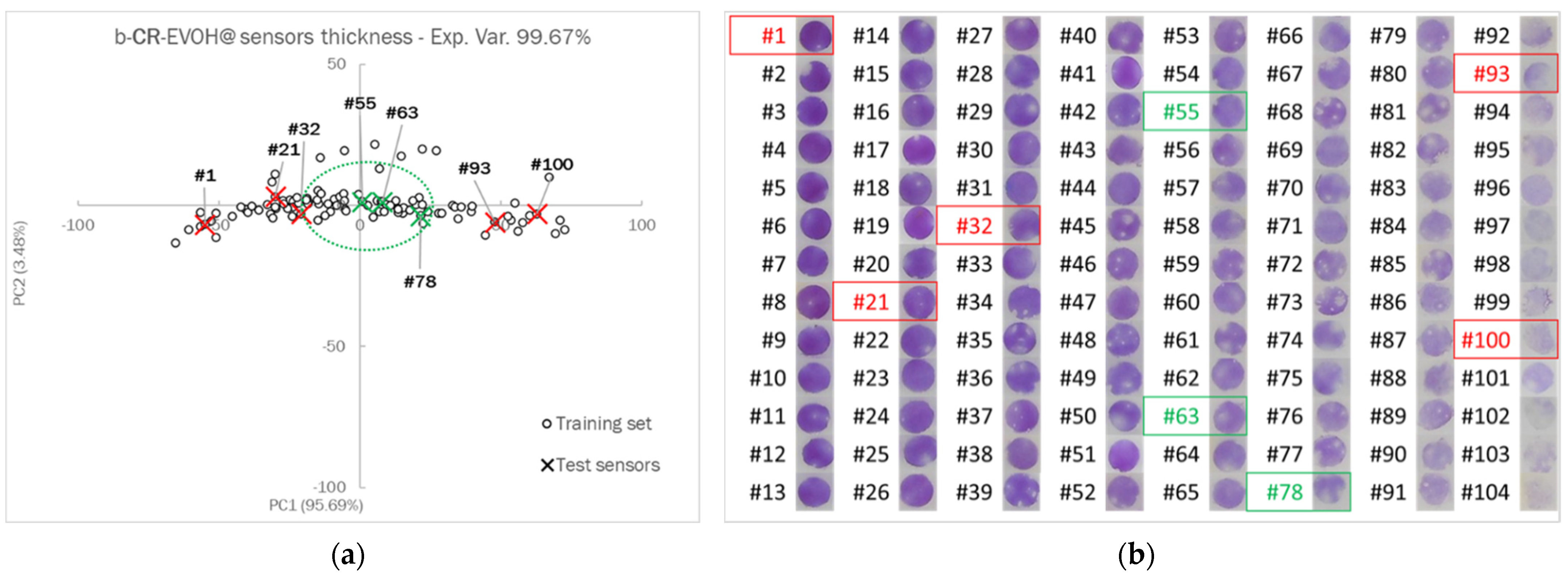
2.2. Sensors Thickness Selection

EVOH copolymers characterized by high MFR resulted in films with less homogeneous thickness, as could be expected. As sensors’ thickness is strongly related to their sensitivity and sensing rate, a rapid method to verify and keep this parameter under control was developed. A large number of sensors with various thicknesses were equilibrated at acid or alkaline, as described above, and, from the sensors’ pictures, RGB triplets were extrapolated and used as the input dataset for PCA. Then, a few sensors, representative of the various thicknesses, were selected and tested on real samples to evaluate the most effective thickness for the final application. The suitable thickness range was thus identified, and only sensors within this interval were used for vapor analysis.

2.3. Experimental Set-Up for Vapors Analysis

Dye-EVOH@ sensors were tested for the detection of acid–base analytes in vapor phase, released both by synthetic and real samples, in closed containers of defined volume. The procedure for volatile analyte detection consists of two steps: first, Dye-EVOH@ sensors were equilibrated at a specific acid–base form by 1-hour immersion of each sensor in 2 mL NaOH or HNO3 0.1 M, whether the detection of respectively acidic or alkaline analytes is required. Then, sensors were rinsed with water and dried on paper. Second, the sensors were fixed on an adhesive strip, placed forming a sort of bridge taped to closed container walls so that the sensing units make contact only with the headspace and never with the samples. To avoid the undesirable reaction of the sensors with the acid–base components of the adhesive strip, several commercial tapes had been previously tested and 3 M Magic Tape had been identified as inert [26,27,28,29].
As for synthetic samples, ammonia and acetic acid were selected as vapors-generating solutions, respectively alkaline and acid, due to their volatility; the vapor analysis was performed at different solution concentrations and storage temperatures to test the sensors’ sensitivity. Next, 50 mL of NH3 and CH3COOH solutions at various concentrations (0.1 M and 0.01 M) were poured into a plastic box (16.5 cm × 10.5 cm × 6 cm; 2 L), sensors were located in the box headspace, the container was sealed by food-grade plastic film and pictures of the sensors were acquired at fixed times, storing the box at 22 or 4 °C. Obviously, sensors were equilibrated at alkaline pH, i.e., violet color (b-CR-EVOH@), to detect acidic analytes and at acidic pH, i.e., pink color (a-CR-EVOH@), to detect alkaline species. A picture of this experimental setup is reported in Figure S1a. The same experimental setup was also used to test the sensors’ colour stability in the absence of acid–base analytes, substituting vapor-generating solutions with phosphate buffer (pH = 7).
As for real samples, chicken breast slices were used as test protein food to verify the applicability of the sensors for freshness monitoring. Chicken breast slices of similar weights (around 300 g) were purchased at the local supermarket and carried to the laboratory within 10 min. The sensors were located directly inside the sales package (22.5 cm × 16 cm × 2.5 cm; V~0.9 L) which was sealed by food-grade plastic film. To better mimic home conditions, chicken samples were stored in a domestic fridge at 4 °C for 10 days, and pictures of the sensors were acquired 2 or 3 times per day until complete degradation. In this case, being interested in jointly detecting acidic and alkaline volatile by-products, a dual-sensor array was used, made up of one sensor equilibrated at alkaline pH, i.e., the sensor in its violet fully deprotonated color (b-CR-EVOH@), and one at acidic pH, i.e., the sensor in its pink fully protonated color (a-CR-EVOH@), to detect alkaline species. A picture of this experimental setup is reported in Figure S1b.

2.4. Pictures Acquisition and Multivariate Data Elaboration

Pictures of the sensors were taken by a NIKON COOLPIX S6200 portable camera equipped with a 1/2.3” (6.16 mm × 4.62 mm, crop factor 5.6) 16 mpx CCD sensor. A portable led lightbox (23 cm × 23 cm × 23 cm), equipped with 20 LEDs (550LM, colour temperature 5500 K) was used to guarantee the reproducibility of the photos (PULUZ, Photography Light Box, Shenzhen Puluz Technology Limited, Shenzhen, China). A picture of the lightbox is shown in Figure S2.
Setting ISO at the lowest possible for the camera (80) and using the lightbox, all the pictures were acquired at shutter speed 1/60 s and aperture f/3.2. The white balance was kept constant for all the images by setting a white reference point inside the lightbox. The pictures (4608 × 3456 pixels) were acquired as a .jpg file using a neutral photo profile from the camera. GIMP software was used to acquire the RGB triplets from the .jpg files straight from the camera, manually selecting the region of interest (ROI) by exploiting the “Intelligent Scissors” tool. [36]
In addition to naked-eye evaluation, RGB triplets were submitted to principal component analysis (PCA) to rationalize the colour evolution during the vapor analysis. Since RGB indexes are intrinsically scaled between 0 and 255, centering was the only pretreatment exploited. The chemometric elaborations were performed using the open-source software Chemometric Agile Tool (CAT) [37].
Both in the case of vapor analysis performed using synthetic and real samples, PCA outputs were firstly evaluated and then the score values were plotted vs. time to better highlight the kinetic of analytes detection and to jointly analyze the preliminary corroboration results.

2.5. TVB-N Quantification

TVB-N values were determined by adapting the method reported by the European Commission Regulation, as widely proposed in the literature [38,39]. The sample to be analyzed was ground carefully by a grinder; 10 g of the ground sample were weighed in a suitable container, mixed with 90 mL of 6% perchloric acid solution, homogenized for two minutes with a blender and then filtered. Steam distillation of 50 mL of the extract after sufficient alkalinization with 20% NaOH (6.5 mL) controlled by the pink color change of several drops of phenolphthalein (1 g/100 mL 95% ethanol) began immediately. The distillation out-flow tube was submerged in a receiver with 100 mL boric acid solution, 3% to which five drops of the indicator solution, Tashiro Mixed Indicator (0.2 g methyl red and 0.1 g methylene blue are dissolved in 100 mL 95% ethanol), were added. The distillation was ended when 100 mL extract was collected. The volatile bases contained in the receiver solution were determined by titration with standard hydrochloric solution 0.01 M until the colour of the Tashiro Mixed Indicator changed from green/blue to violet.
This procedure was performed on three replicates at Day 1, 4, 8 and 10 and TVB-N values, expressed as mg/100 g of chicken meat, were calculated according to Equation (S1), reported in the Supplementary Materials. The results obtained are perfectly in agreement with the values found in the literature, as summarized by Bekhit and coworkers [38].

2.6. Microbiological Analysis

Microbiological analysis was performed according to European Commission Regulations. [40] The minced meat samples were portioned into 4 packs of 150 g and stored at 4 °C ± 1. During this preliminary phase, the samples were analyzed at different times, chosen based on the results reported in the following section. The microbiological analysis was carried out on the same day of packaging (Day 1) and after 5 (Day 5), 8 (Day 8) and 10 (Day 10) days. Specifically, 25 g of the sample were diluted in Ringer’s solution and homogenized in a Stomacher device (Lab Blender 400, Seward Medical, Worthing, UK) for 120 s at room temperature. The microbial load was evaluated using serial decimal dilution in Ringer, and 0.1 mL of the appropriate dilution was spread on plate count agar (PCA) medium and incubated at 37 °C for 48 h. The results were logarithmically transformed and expressed as log colony-forming unit (CFU)/g.

3. Results and Discussion

3.1. Sensing Approach for 3-Step Degradation Detection

As hinted before, animal-based protein food degradation can be divided into three main steps, freshness (F), early spoilage (ES) and spoilage (S), which are characterized by the bacterial release of by-products with different acid–base behaviors and volatility. Immediately after animal death, bacterial activity leads to the production and release of volatile fatty acids in the package headspace, provoking an ever-increasing acidity in the atmosphere; considering the low toxicity of these compounds and always bearing in mind the large-scale application, it is pointless to detect the beginning of acidic volatile by-products release, which occurs in the very first step of degradation (F).
Nevertheless, the detection of these analytes turns out to be interesting when high amounts of acids are released, which means when the early spoilage (ES) is ongoing and food is still eatable but no longer fresh; for this reason, our idea is to detect only considerable amounts of acidic by-products using one pH indicator with a logKa value slightly above 7, equilibrated at alkaline form, which shows a complete transition to the neutral form only when the environment is definitely acidic.
Oppositely, during spoilage (S), an assortment of amines is released, characterized by different dimensions, molecular weights and acid–base behaviors among which only a few are actually volatile, mainly NH3. For instance, the most significant class of amines, in terms of toxicity, is represented by biogenic amines (BA), but these molecules, at the buffered pH typical of foodstuffs, are protonated and cannot pass into the vapor phase [41]. Having this problem clear in our minds, the only way to detect the production of toxic by-products, occurring during the third step (S), is to exploit a pH indicator extremely sensitive towards alkaline molecules, ideally with logKa value much below 7, equilibrated at acidic form, which shows a complete transition to the neutral form even in the presence of very low concentrations of volatile amines.

3.2. Sensors’ Components Selection

Considering the paramount importance of sensitivity tuning required for freshness sensors, a panel of Dye-EVOH@ sensors was synthesized, including commercial EVOH copolymers with different monomers ratios and MFR and, thus, properties [42] and sulfonphthaleins with various logKa values. Both the solid supports and the dyes under investigation are listed in the Supplementary Materials (Tables S1 and S2). Having defined our target sensing approach, described above, the smartest way to select both the receptors and the solid support is to test all the candidates directly on chill-stored protein foods.
These screening experiments, whose most prominent results are reported in Figures S3 and S4, led to the selection of EVOH copolymer with 29% ethylene content and MFR = 8 as the most permeable and thus sensitive material, particularly for the early detection of the spoilage step, characterized by toxic by-products. As for the receptor, the choice fell on o-cresol red (CR), since this pH indicator is involved in two protonation equilibria, one at slightly alkaline and one at extremely acidic pH, and thus, depending on the pH of equilibration, it could ensure both ES and S detection. The logKa values in solution for this molecule are reported in the literature [43,44], but it must be underlined that, after the covalent linkage to EVOH, an increase of around 1 unit for each log Ka value is observed [29,30,31]. In Figure 1, the protonation equilibria with the corresponding logKa values and color shade, both in solution and after functionalization, are reported. Further investigation of this aspect is still ongoing.

3.3. Sensors Effective Thickness Selection

As is thoroughly discussed in the literature [45], MFR influences thermoplastic polymers’ behavior during both pressing and extrusion; in fact, the selection of an EVOH copolymer with high MFR results in sensitive films with ununiform thickness. It being impossible to avoid or control this issue by changing the pressing parameters and considering the strict correlation between sensors’ thickness, sensitivity and sensing rate, a rapid method to select only sensors with suitable thickness is developed. We must not forget that EVOH is industrially used as barrier film and, obviously, the thickness of EVOH films affects their permeability and, in this case, the diffusion rate of volatile by-products within the polymer matrix and, thus, the receptors’ detection and colour change. Both weighing each sensor and measuring each one’s thickness using a profilometer are discarded as control strategies, respectively resulting in the sensors having too low of an average mass and requiring too much experimental effort, while exploiting the relationship between sensors’ thickness and colour intensity represents a much quicker and more reliable approach.
Therefore, a large panel of CR-EVOH@ sensors was made up to investigate the widest range of thicknesses; part of it was equilibrated at acidic pH and part at alkaline pH, because these two sensors are required for real sample analysis. Sensors’ RGB triplets were collected and used as input datasets for PCA to reduce the data’s dimensionality and obtain a single parameter representative of sensor thickness [31]. As an example, the case of sensors equilibrated at alkaline pH is shown in Figure 2, while the other case is reported in the Supplementary Materials (Figures S5b and S6). In the PCA score plot, shown in Figure 1a, the sensors are ordered alongside PC1 (99.67% explained variance) with the lower score value of PC1 associated with the higher sensor thickness, as clearly highlighted in the loading plots in Figure S5a. Thus, the score value on PC1 can be used to measure sensor thickness, both for the training set and any other following sensor, by projection in the score plot.
Once having summarized this information in one single parameter, the most effective thickness range is identified by testing the CR-EVOH@ sensors directly on chill-stored protein foods, following the approach previously described. Therefore, from the starting sensors reported in Figure 2b, ordered by increasing score on PC1 and thus by decreasing thickness, 8 sensors representative of various thicknesses were selected and used in preliminary real sample monitoring. Three out of the eight sensors, highlighted in green in Figure 2a,b, presented a suitable color transition during chicken breast slices’ freshness monitoring, being neither too thick to react slowly with the analytes nor too thin to exhibit faded colors.

3.4. Detection Kinetic of Acid–Base Analytes in Vapor Phase

Once the best solid support and receptor and the effective thickness range were defined, the sensing performances of CR-EVOH@ sensors towards acid or alkaline analytes in vapor phase were evaluated. As described in Section 2.3, ammonia and acetic acid were selected as vapor-generating synthetic samples, the experimental set-up, in terms of solution and container volume and sensor location, is kept constant, while the concentration of ammonia and acetic acid and the storage temperature is decreased to evaluate the sensors’ sensitivity.
In Figure S7, the pictures of CR-EVOH@ sensors acquired during vapor analyses are displayed. As expected and required, the sensitivity shown by CR-EVOH@ equilibrated at acidic pH, from now named a-CR-EVOH@, towards alkaline analytes is higher than the one presented by CR-EVOH@ equilibrated at alkaline pH, from now named b-CR-EVOH@, towards acidic analytes. This very first result confirms the suitability of CR-EVOH@ to detect both ES and S, depending on the equilibration.
For a systematical investigation of sensors sensitivity and sensing rate, RGB triplets’ trends were rationalized by PCA, and the score values on PC1, which account for more than 85% of explained variance in most cases, were exploited as parameter representative for analyte detection by color change. For brevity’s sake, the % explained variance, the loading and score values for each vapor analysis are reported, respectively, in Table S4 and Figure S8 in the Supplementary Materials. To compare detection kinetics for different analytes concentrations, considering that PCA leads to soft models and thus score values cannot be directly compared, per each vapor analysis the normalized Euclidean distance (nED) between PC1 score value at given time and at the end of the analyses was calculated according to Equation (S2). In Figure 3, nED vs. time plots are displayed in the case of ammonia (Figure 3a) and acetic acid (Figure 3b) at different concentrations and temperatures. This data treatment may sound a bit laborious, but it led to easy-to-interpret kinetic curves, similar to those typically obtained by kinetic experiments even if relying on multivariate data treatment.
As is clearly visible in Figure 3a, the a-CR-EVOH@ sensor exhibits huge sensitivity towards ammonia and no significant kinetic slowdown was observed lowering the analytes concentration or the temperature, while b-CR-EVOH@ detection of acetic acid in vapor phase (Figure 3b) is slower and further decreased by lowering the concentration or the temperature. Apart from slight differences in analytes volatility, the main reason for the different kinetics and relationship between detection rate and concentration has to be found in the protonation equilibria: ammonia detection is performed by exploiting a protonation equilibrium occurring at a definitely acidic pH, as highlighted in Figure 1, and therefore a distinctly low amount of NH3 in vapor phase can provoke a complete colour change while, on the other hand, acetic acid detection relies on a protonation equilibrium occurring at a slightly alkaline pH, and a higher concentration of AcOH is required to obtain the complete color transition. Therefore, this analysis has to be read as a further demonstration of the suitability of CR-EVOH@ sensors for 3-step degradation monitoring.

3.5. Sensors’ Stability

Before sensors’ application on real samples, not only sensors’ sensitivity toward the target analytes but also sensors’ stability in the absence of analytes must be checked to avoid, respectively, both false-negative and false-positive results. In this case, the stability of both b-CR-EVOH@ and a-CR-EVOH@ is checked, using the same experimental set-up used for vapor analyses but replacing vapor-generating solutions with phosphate buffer. Pictures of both the sensors, acquired over 10 days, similarly to the real food monitoring, are reported in Figure S9: no difference can be observed in the sensors’ color during the time range investigated, thus confirming the stability of the sensors in the absence of analytes.

3.6. Application on Real Samples: Chicken Breast Slices Freshness Monitoring during Chilled Storage

After the characterization step, both of the CR-EVOH@ sensors were collected in a sensor array made of one b-CR-EVOH@ and one a-CR-EVOH@ sensing unit and tested for the detection of 3-step spoilage in chicken breast slices under chilled storage. The experiments were performed using five samples of similar mass purchased on the same day as the delivery from the supplier, according to the procedure reported in Section 2.3. Then, two new samples of similar mass were used as a test set, one purchased the same day as the delivery and the other two days after. This test aims to verify the correct device behavior even if implemented in foods already under degradation.
In Figure 4a, the array pictures, acquired two or three times per day during the degradation of the training set, are displayed, while the pictures of the test set are reported in Figure S10. For this specific application, naked-eye analysis of colour evolution represents a crucial step since, aiming at a large-scale implementation in food packaging, such a device must be readable also for untrained consumers, without the need for applications or readers. Therefore, the device has to show a clear and glaring colour transition according to headspace composition and thus food freshness.
From a naked-eye evaluation of Figure 4a, we can observe that the sensors’ colour remained unchanged for the first three days, in correspondence with the first degradation step, labelled as freshness (F). Then, during early spoilage (ES), the high amount of weak acid volatile by-products, which bacteria had been releasing since animal death, was detected by b-CR-EVOH@ which turned its colour from violet (CR-) to yellow (HCR) between Day 4 and Day 6, with a slightly different timing between the replicates due to the intrinsic variability of foods under investigation. Finally, when spoilage (S) began, the release of thiols and amines was immediately detected by a-CR-EVOH@ changing its colour from pink (H2CR+) to yellow (HCR) within Day 7 and 9.
To rationalize the sensors’ color evolution, at every acquisition time RGB triplets were acquired, as described before, and the overall matrix of 6 columns (3 RGB indexes per 2 CR-EVOH@ sensors) and 135 rows (27 acquisition times per 5 replicates) was submitted to PCA, only centering the data. The model was built considering the first two principal components which together explain 93.7% of the variance (85.43% PC1, 8.26% PC2); the loading values on these two components are reported in the histogram in Figure S11, for brevity’s sake.
The score plot, shown in Figure 4b, perfectly rationalizes the sensors’ behavior as previously described. PC1, which accounts for the main % explained variance, generally represents the ongoing spoilage process; the samples’ score values on the x-axis increase during spoilage, with a more evident increase during ES between Day 4 and 6, in conjunction with the b-CR-EVOH@ color transition from violet to yellow. PC2, instead, is specifically related to the S step, occurring between Day 7 and Day 10, since in this time-lapse, samples’ score values on PC1 slightly increase while the PC2 values significantly decrease. This interpretation is supported by the loading values reported in Figure S11.
As for test set projection, the new samples acquired the same day of the delivery from the supplier, represented as black diamonds in Figure 4b, show a similar degradation process and are correctly located in the score plot. Opposite, projecting the test sample acquired two days after the delivery (blue diamond), the sensor array detects the lower freshness of the food and, as spoilage goes on, a shift of two days is observed in the location of the sample in the score plot, with the test sample at Day 3 aligned on PC1 to training samples at Day 5 and so on.
To make even clearer the sensors’ color evolution and the consequent spoilage process, hinted by naked-eye evaluation and rationalized by PCA, the average score values on PC1 and PC2 for the five samples of the training set at each acquisition time were calculated and plotted vs. time, expressed in hours, together with the respective standard deviations, as displayed in Figure 4c. The corresponding sensor array’s coloration at each step is added in Figure 4c to ease the comprehension of the results presented. Three steps are clearly highlighted in this plot:
  • Freshness (F): both the PC1 and PC2 score values remain constant, meaning that none of the sensors is changing its color (Day 1–Day 3). In this step, the dual-sensor array still presents its starting coloration—violet for b-CR-EVOH@ and pink for a-CR-EVOH@.
  • Early spoilage (ES): PC1 score values undergo a steady increase related to b-CR-EVOH@ color transition from violet to yellow as a consequence of acidic volatile by-products’ detection (Day 4–Day 6). A slight increase is observed also for PC2 score values.
  • Spoilage (S): PC1 score values’ increase becomes much less evident, while PC2 score values significantly lower as a consequence of a-CR-EVOH@ detection of a slightly more alkaline environment, and consequently, the color turns from pink to yellow. (Day 7–10).

3.7. CR-EVOH@ Dual-Sensor Array Corroboration

Projection of unknown test samples was exploited as a very first attempt at PCA model corroboration, but the correlation between sensor array color evolution and food samples’ freshness must be verified by independent methods. To fulfil this aim, two different approaches are followed. On one hand, TVB-N is determined on three replicates at a given time during degradation, being the most common chemical parameter applied to evaluate the quality of fish and other meat products [38,39]. The TVB-N average values and correspondent standard deviations calculated on three independent samples per each measurement time, determined during chicken breast slices’ spoilage, are reported in Figure 5a.
Before commenting on the results, it must be underlined that in the literature, an agreement on TVB-N value to be considered as the freshness threshold for chicken meat was still not found. As perfectly summarized in a recent review by Bekhit and coworkers [38], in different papers the TVB-N values of 15, 23, 25 and 28 mg/100 g are used as the threshold to evaluate chicken freshness. As for the European Regulation, up to our knowledge, the threshold values are reported only for fish and fishery products and not for other types of protein foods [39]. Having this issue in our mind, we can only give a qualitative judgment on TVB-N trend during spoilage. On the first day of monitoring, when food is definitely fresh, TVB-N value is around 6, which is far below the range of threshold values; at Day 4, at the beginning of ES, an increase to around 15 is observed, which means near to the threshold values proposed in the literature, but higher growth is found at Day 8, when TVB-N value exceeds 26, and at Day 10 (TVB-N higher than 36). These two last measurements definitely confirmed the occurred spoilage of the chicken meat, being above all the threshold values proposed in the literature. Therefore, the TVB-N trend seems to confirm sensors’ behavior, even if it must be underlined that amines included in TVB-N are all those N-containing compounds extracted and purified via steam distillation in alkaline conditions [30]. This means that this parameter includes a wider panel of amines than the actual volatile ones at food-buffered pH, which are the ones that could be detected by the sensor array [30].
On the other hand, a total viable counts (TVCs) analysis was performed. This preliminary test was performed as a “proof of concept” to check if a correlation could be found between the sensor array and TVCs average values, as reported in Figure 5b. TVCs ranges from around 3 log CFU/g at Day 1, to around 6 log CFU/g at Day 5, confirming the transition from a fresh to an early spoilt sample. Then, at Days 8 and 10, the TVCs value rises above 8 CFU/g, higher than the acceptability limit set at 7 CFU/g [46], with only a slight increase between the two measurements, confirming the ongoing spoilage step and thus the samples’ unsuitability for human consumption. It must be underlined that, in this preliminary assay, the different bacterial populations forming the SSO are not investigated, since only the TVCs are determined. Considering the encouraging results, further experiments will be performed to seek a direct correlation between CR-EVOH@ device color evolution and the activity of specific bacterial populations.

4. Conclusions

Starting from a cheap commercial pH indicator and one of the most-used polymers in food packaging, we succeeded in the development of an efficient smart label prototype. The proposed device is able to distinguish the three main degradation steps poultry meat experiences, i.e., freshness, early spoilage and spoilage, and the recognition of the current step can be performed at a glance, by a simple naked-eye readout, by untrained people. Furthermore, the device showed similar colour evolution for different samples purchased in different moments, even if always in the same supermarket.
In addition to naked-eye analysis, multivariate analysis allows for extracting more information, visualizing and rationalizing the spoilage process and corroborating the device responses. Exploiting three different approaches for the preliminary corroboration turned out to be the winning choice, since we were able to demonstrate the correct freshness detection on unknown independent samples, the correlation between our sensors’ color evolution and both the N-containing compounds released during bacterial degradation and the microorganisms’ proliferation in the food.
Last but not least, the proposed device represents an eligible candidate to exit the laboratory and reach the supermarket shelf thanks to its extremely low cost of production, estimated below 0.10 €, the scalable production procedures and the easy implementation in food packages, as the device is substantially made of the same polymeric mate-rial and suitable for heat-sealing on food-grade plastic films. All these pros, together with the strong scientific background, the deep comprehension of spoilage mechanisms and by-products’ distribution in the package and the possibility of an easy naked-eye detection, are currently the most appreciated features by food supply chain players and operators.
As a matter of fact, the applicability of the device has been widely demonstrated for chicken samples stored only at 4 °C, but further investigations regarding different storage temperatures are actually ongoing.

Supplementary Materials

The following supporting information can be downloaded at: https://www.mdpi.com/article/10.3390/appliedchem2030009/s1, Table S1: Commercial EVOH copolymers under investigation with their ethylene content and MFR; Table S2: Commercial sulfonphthalein pH indicators tested and their logKa as found in literature; Table S3: Optimized pressing parameters for Dye-EVOH@; Figure S1: Experimental setup for vapor analysis using synthetic samples; Figure S2: Picture of the light box employed to take array photographs; Equation (S1): TVB-N calculation; Figure S3: Color evolution over codfish fillets, stored at 4 °C, of Dye-EVOH@ sensors arrays, using EVOH A, B, C and D as solid support; Figure S4: Color evolution over chicken breast slices, stored at 4 °C, of Dye-EVOH@ sensors arrays, using EVOH B; Figure S5: PCA loading plots of the first two components based on RGB triplets of 104 b-CR-EVOH@ (a) and 132 a-CR-EVOH@ (b) sensors of various thicknesses; Figure S6: PCA score plot of the first two components based on RGB triplets of 132 sensors of various thicknesses (white circles); Figure S7: Color evolution of a-CR-EVOH@ sensors over ammonia solutions (a) and of b-CR-EVOH@ over acetic acid solutions (b); Table S4: % Explained variance on PC1, PC2 and PC1 + PC2 per each vapor analysis performed; Figure S8: Loading and score plots on the first two principal components for acid and alkaline vapors analyses; Equation (S2): Normalized Euclidean Distance calculations; Figure S9: Colour evolution of CR-EVOH@ dual-sensor array exposed to 50 mL phosphate buffer (pH = 7) in a sealed box (1.5 L) during 10-day monitoring at 22 °C and 4 °C; Figure S10: CR-EVOH@ dual-sensor array colour evolution over chicken breast slice samples, belonging to the test set; Figure S11: PCA loading plot on the first two principal components for chicken breast slices’ freshness.

Author Contributions

Conceptualization, L.R.M. and R.B.; validation, E.B. and J.H.S.; formal analysis, L.R.M. and C.Z.; investigation, L.R.M.; writing—original draft preparation, L.R.M.; writing—review and editing, G.A., P.Q. and R.B. All authors have read and agreed to the published version of the manuscript.

Funding

This research received no external funding.

Institutional Review Board Statement

Not applicable.

Informed Consent Statement

Not applicable.

Data Availability Statement

Not applicable.

Acknowledgments

We thank MIUR for funding Camilla Zanoni’s PhD grant, and “VIPCAT–Value Added Innovative Protocols for Catalytic Transformations” project (CUP: E46D17000110009) for valuable financial support.

Conflicts of Interest

The authors declare no conflict of interest.

References

  1. Lavigne, J.J.; Anslyn, E.V. Sensing A Paradigm Shift in the Field of Molecular Recognition: From Selective to Differential Receptors. Angew. Chem. Int. Ed. 2001, 40, 3118–3130. [Google Scholar] [CrossRef]
  2. Diehl, K.L.; Anslyn, E.V. Array sensing using optical methods for detection of chemical and biological hazards. Chem. Soc. Rev. 2013, 42, 8596. [Google Scholar] [CrossRef] [PubMed]
  3. Li, Z.; Askim, J.R.; Suslick, K.S. The Optoelectronic Nose: Colorimetric and Fluorometric Sensor Arrays. Chem. Rev. 2019, 119, 231–292. [Google Scholar] [CrossRef] [PubMed]
  4. Fan, Y.; Li, J.; Guo, Y.; Xie, L.; Zhang, G. Digital image colorimetry on smartphone for chemical analysis: A review. Measurement 2021, 171, 108829. [Google Scholar] [CrossRef]
  5. Goncalves Dias Diniz, P.H. Chemometrics-assisted color histogram-based analytical systems. J. Chemom. 2020, 34, 3242. [Google Scholar] [CrossRef]
  6. Lopez-Ruiz, N.; Curto, V.F.; Erenas, M.M.; Benito-Lopez, F.; Diamond, D.; Palma, A.J.; Capitan-Vallvey, L.F. Smartphone-Based Simultaneous pH and Nitrite Colorimetric Determination for Paper Microfluidic Devices. Anal. Chem. 2014, 86, 9554–9562. [Google Scholar] [CrossRef]
  7. Wencel, D.; Abel, T.; McDonagh, C. Optical Chemical pH Sensors. Anal. Chem. 2014, 86, 15–29. [Google Scholar] [CrossRef]
  8. Hoang, A.T.; Cho, Y.B.; Kim, Y.S. A strip array of colorimetric sensors for visualizing a concentration level of gaseous analytes with basicity. Sens. Actuators B Chem. 2017, 251, 1089–1095. [Google Scholar] [CrossRef]
  9. Kim, S.D.; Koo, Y.; Yun, Y. A Smartphone-Based Automatic Measurement Method for Colorimetric pH Detection Using a Color Adaptation Algorithm. Sensors 2017, 17, 1604. [Google Scholar] [CrossRef] [Green Version]
  10. Craig, R.L.; Peterson, P.K.; Nandy, L.; Lei, Z.; Hossain, M.A.; Camarena, S.; Dodson, R.A.; Cook, R.D.; Dutcher, C.S.; Ault, A.P. Direct Determination of Aerosol pH: Size-Resolved Measurements of Submicrometer and Supermicrometer Aqueous Particles. Anal. Chem. 2018, 90, 11232–11239. [Google Scholar] [CrossRef]
  11. Duong, H.D.; Shin, Y.; Rhee, J.I. Development of novel optical pH sensors based on coumarin 6 and nile blue A encapsulated in resin particles and specific support materials. Mater. Sci. Eng. 2020, 107, 110323. [Google Scholar] [CrossRef] [PubMed]
  12. Pastore, A.; Badocco, D.; Cappellin, L.; Pastore, A. Enhancement of the pH measurement of a PVDF-supported colorimetric sensor by tailoring hue changes with the addition of a second dye. Microchem. J. 2020, 154, 104552. [Google Scholar] [CrossRef]
  13. Li, G.; Su, H.; Ma, N.; Zheng, G.; Kuhn, U.; Li, M.; Klimach, T.; Pöschl, U.; Cheng, Y. Multifactor colorimetric analysis on pH-indicator papers: An optimized approach for direct determination of ambient aerosol pH. Atmos. Meas. Tech. 2020, 13, 6053–6065. [Google Scholar] [CrossRef]
  14. Balbinot-Alfaro, E.; Vieira Craveiro, D.; Oliveira Lima, K.; Leão Gouveia Costa, H.; Rubim Lopes, D.; Prentice, C. Intelligent Packaging with pH Indicator Potential. Food Eng. Rev. 2019, 11, 235–244. [Google Scholar] [CrossRef]
  15. Müller, P.; Schmid, M. Intelligent Packaging in the Food Sector: A Brief Overview. Foods 2019, 8, 16. [Google Scholar] [CrossRef] [Green Version]
  16. Alizadeh-Sani, M.; Mohammadian, E.; Rhim, J.-W.; Jafari, S.M. pH-sensitive (halochromic) smart packaging films based on natural food colorants for the monitoring of food quality and safety. Trends Food Sci. Technol. 2020, 105, 93–144. [Google Scholar] [CrossRef]
  17. Priyadarshi, R.; Ezati, P.; Rhim, J.-W. Recent Advances in Intelligent Food Packaging Applications Using Natural Food Colorants. ACS Food Sci. Technol. 2021, 1, 124–138. [Google Scholar] [CrossRef]
  18. Rodrigues, C.; Lauriano Souza, V.G.; Coelhoso, I.; Fernando, A.L. Bio-Based Sensors for Smart Food Packaging—Current Applications and Future Trends. Sensors 2021, 21, 2148. [Google Scholar] [CrossRef]
  19. Dodero, A.; Escher, A.; Bertucci, S.; Castellano, M.; Lova, P. Intelligent Packaging for Real-Time Monitoring of Food-Quality: Current and Future Developments. Appl. Sci. 2021, 11, 3532. [Google Scholar] [CrossRef]
  20. Kuswandi, M.; Nurfawaidi, A. On-package dual sensors label based on pH indicators for real-time monitoring of beef freshness. Food Contr. 2017, 82, 91–100. [Google Scholar] [CrossRef]
  21. Mikš-Krajnik, M.; Yoon, Y.-J.; Yuk, H.-G. Detection of volatile organic compounds as markers of chicken breast spoilage using HS-SPME-GC/MS-FASST. Food Sci. Biotechnol. 2015, 24, 361–372. [Google Scholar] [CrossRef]
  22. Mikš-Krajnik, M.; Yoon, Y.-J.; Ukuku, D.O.; Yuk, H.-G. Identification and Quantification of Volatile Chemical Spoilage Indexes Associat-ed with Bacterial Growth Dynamics in Aerobically Stored Chicken. J. Food Sci. 2016, 81, M2006–M2014. [Google Scholar] [CrossRef] [PubMed]
  23. Nychas, G.-J.E.; Skadamis, P.N.; Tassou, C.C.; Koutsoumanis, K.P. Meat spoilage during distribution. Meat Sci. 2008, 78, 77–89. [Google Scholar] [CrossRef] [PubMed]
  24. Dainty, R.H. Chemical/biochemical detection of spoilage. Int. J. Food. Microbiol. 1996, 33, 19–33. [Google Scholar] [CrossRef]
  25. Erim, F.B. Recent analytical approaches to the analysis of biogenic amines in food samples. Trends Analyt. Chem. 2013, 52, 239–247. [Google Scholar] [CrossRef]
  26. Magnaghi, L.R.; Alberti, G.; Quadrelli, P.; Biesuz, R. Development of a dye-based device to assess the poultry meat spoilage. Part I: Building and testing the sensitive array. J. Agric. Food Chem. 2020, 68, 12702–12709. [Google Scholar] [CrossRef]
  27. Magnaghi, L.R.; Alberti, G.; Capone, F.; Zanoni, C.; Mannucci, B.; Quadrelli, P.; Biesuz, R. Development of a dye-based device to assess the poultry meat spoilage. Part II: Array on act. J. Agric. Food Chem. 2020, 68, 12710–12718. [Google Scholar] [CrossRef]
  28. Magnaghi, L.R.; Capone, F.; Zanoni, C.; Alberti, G.; Quadrelli, P.; Biesuz, R. Colorimetric sensor array for monitoring, modelling and comparing spoilage processes of different meat and fish foods. Foods 2020, 9, 684. [Google Scholar] [CrossRef]
  29. Magnaghi, L.R.; Alberti, G.; Milanese, C.; Quadrelli, P.; Biesuz, R. Naked-Eye Food Freshness Detection: Innovative Polymeric Optode for High-Protein Food Spoilage Monitoring. ACS Food Sci. Technol. 2021, 1, 165–175. [Google Scholar] [CrossRef]
  30. Magnaghi, L.R.; Capone, F.; Alberti, G.; Zanoni, C.; Mannucci, B.; Quadrelli, P.; Biesuz, R. EVOH-based pH-sensitive Optodes Array & Chemometrics: From Naked-eye Analysis to Predictive Modelling to Detect Milk Freshness. ACS Food Sci. Technol. 2021, 1, 819–828. [Google Scholar] [CrossRef]
  31. Magnaghi, L.R.; Zanoni, C.; Alberti, G.; Quadrelli, P.; Biesuz, R. Towards intelligent packaging: BCP-EVOH@ optode for milk freshness measurement. Talanta 2022, 241, 123230. [Google Scholar] [CrossRef] [PubMed]
  32. Biesuz, R.; Quadrelli, P.; Magnaghi, L.R. Sensori per la Valutazione della Qualità di Prodotti Alimentari a Base di Carne. Italian Patent 10201900000464, 19 March 2019. [Google Scholar]
  33. Biesuz, R.; Quadrelli, P.; Magnaghi, L.R. Sensors for the Evaluation of the Quality of Meat-Based Food. WIPO PCT/IB2020/052998, 30 March 2020. [Google Scholar]
  34. Biesuz, R.; Quadrelli, P.; Magnaghi, L.R. Sensors for the Evaluation of the Quality of Meat-Based Food. U.S. Patent 17599196, 28 September 2021. [Google Scholar]
  35. Biesuz, R.; Quadrelli, P.; Magnaghi, L.R. Sensors for the Evaluation of the Quality of Meat-Based Food. EURO-PCT 20721299.4, 30 March 2020. [Google Scholar]
  36. GNU Image Manipulation Program (GIMP). Available online: https://www.gimp.org/ (accessed on 1 January 2022).
  37. Leardi, R.; Melzi, C.; Polotti, G. CAT (Chemometric Agile Tool). Available online: http://www.gruppochemiometria.it/index.php/software/19-download-the-rbased-chemometric-software (accessed on 1 January 2022).
  38. Bekhit, A.E.-D.A.; Holman, B.W.B.; Giteru, S.G.; Hopkins, D.L. Total volatile basic nitrogen (TVB-N) and its role in meat spoilage: A review. Trends Food Sci. Technol. 2021, 109, 280–302. [Google Scholar] [CrossRef]
  39. European Commission Regulation (EC) No 2074/2005 of 5 December 2005. Total volatile basic nitrogen (TVB-N) limit values for certain categories of fishery products and analysis methods to be used. Off. J. Eur. Union 2005, 338, 36–39.
  40. European Commission Regulation (EC) No. 2073/2005, Microbiological criteria for foodstuffs. Off. J. Eur. Union 2005, 338, 1.
  41. Biesuz, R.; Magnaghi, L.R. Role of Biogenic Amines in Protein Foods Sensing: Myths and Evidence. In Meat and Nutrition; Ranabhat, C.L., Ed.; IntechOpen: London, UK, 2021. [Google Scholar] [CrossRef]
  42. Maes, C.; Luyten, W.; Herremans, G.; Peeters, R.; Carleer, R.; Buntinx, M. Recent Updates on the Barrier Properties of Ethylene Vinyl Alcohol Copolymer (EVOH): A Review. Pol. Rev. 2018, 58, 209–246. [Google Scholar] [CrossRef] [Green Version]
  43. Casula, R.; Crisponi, G.; Cristiani, F.; Nurchi, V.M.; Casu, M.; Lai, A. Characterization of the ionization and spectral properties of sulfonephtalein indicators. Correlation with substituent effects and structural features. Talanta 1993, 40, 1781–1788. [Google Scholar] [CrossRef]
  44. Aragoni, M.C.; Arca, M.; Crisponi, G.; Nurchi, V.M.; Silvagni, R. Characterization of the ionization and spectral properties of sulfonephtalein indicators. Correlation with substituent effects and structural features. Part II. Talanta 1995, 42, 1157−1163. [Google Scholar] [CrossRef]
  45. Riley, A. 14—Plastics manufacturing processes for packaging materials. In Packaging Technology; Emblem, A., Emblem, H., Eds.; Woodhead Publishing: Sawston, UK, 2012; pp. 310–360. [Google Scholar] [CrossRef]
  46. EFSA Panel on Biological Hazards (BIOHAZ). Growth of spoilage bacteria during storage and transport of meat. EFSA J. 2016, 14, 4523. [CrossRef]
Figure 1. Protonation equilibria of o-cresol red (a), color evolution in solution (~10 μM) and correspondent logKa, as found in the literature [33,34] (b) and CR-EVOH@ sensors coloration and apparent logKa after functionalization, estimated from background experiments [29,31,32] (c).
Appliedchem 02 00009 g001
Figure 2. PCA score plot on the first two components based on RGB triplets of 104 sensors of various thicknesses (white circles). The sensors tested for chicken breast slices monitoring are highlighted with green and red Xs, and the suitable thickness range is identified by the green oval (a). Pictures of the 104 sensors used to build the PCA model where sensors tested for chicken breast slices monitoring are highlighted in green and red (b).
Appliedchem 02 00009 g002
Figure 3. Normalized Euclidean distance (nED) between PC1 score values at given time and at the end of the analysis vs. time in the case of a-CR-EVOH@ exploited for ammonia detection (a) and b-CR-EVOH@ for acetic acid detection (b). Both of the vapor-generating compounds were tested at 0.1 M (22 °C) and 0.01 M (22 °C and 4 °C).
Appliedchem 02 00009 g003
Figure 4. CR-EVOH@ dual-sensor array’s color evolution over chicken breast slices stored at 4 °C in the case of training samples; in each array b-CR-EVOH@ is placed on the left and a-CR-EVOH@ on the right (a). PCA score plot of the first two principal components, built on the training set (colored spots) and corroborated by projection of the test sets (black and blue diamonds) for chicken breast slices (b). PC1 (colored spots) and PC2 (colored diamonds) average score values for the training set, as reported in (b) and plotted vs. time in (c).
Appliedchem 02 00009 g004
Figure 5. PC1 (colored spots) and PC2 (colored diamonds) average score values plotted vs. time, as reported in Figure 4c, together with TVB-N values (a) and TVC (b), displayed as, respectively, blue and violet bars. The average values and standard deviations were calculated on three independent samples per each measurement time.
Appliedchem 02 00009 g005
Publisher’s Note: MDPI stays neutral with regard to jurisdictional claims in published maps and institutional affiliations.

