Article

Comparing Methods for Microplastic Quantification Using the Danube as a Model

1
Faculty of Medical and Life Sciences, Institute of Applied Biology, Hochschule Furtwangen, 78054 Villingen-Schwenningen, Germany
2
Department of Earth and Environmental Systems, University of the South, Sewanee, TN 37383, USA
*
Author to whom correspondence should be addressed.
Microplastics 2023, 2(4), 322-333; https://doi.org/10.3390/microplastics2040025
Submission received: 20 August 2023 / Revised: 30 September 2023 / Accepted: 12 October 2023 / Published: 17 October 2023
(This article belongs to the Collection Current Opinion in Microplastics)

Abstract

:
This study investigates the impact different mesh-sized filtration methods have on the amount of detected microplastics in the surface water of the Danube River delta. Further, the distribution of microplastics in different size categories (20 µm, 65 µm, 105 µm) and in the water column (0 m, 3 m, 6 m) was analyzed. Our findings show that the Danube River carries 46 p∙L−1 (microplastic particles per liter) with a size larger than 105 µm, 95 p∙L−1 larger than 65 µm and 2677 p∙L−1 that are larger than 20 µm. This suggests a negative logarithmic correlation between mesh size and particle amount. The most abundant polymer throughout all samples was polyethylene terephthalate, followed by polytetrafluorethylene. Overall, the data shows that different sampling methods cannot be compared directly. Further research is needed to find correlations in particle sizes for better comparison between different sampling methods.

1. Introduction

Due to the fact that plastic is relatively cheap, easy to handle during production, and durable, it is the most often used material in our lives [1]. The widespread utilization of plastic compounds the urgency of the emerging challenges linked to it. Plastic is the catch-all term for a wide range of materials made out of different kinds of synthetic or partially synthetic, non-biodegradable polymers [2]. In our mostly noncircular value chain, the only path a plastic product can take, after its use is deemed over, is to end up in landfills, the ecosystem, or an incineration plant. With 31% of all discarded plastic ending up in landfills and 39% being incinerated in Europe, it is estimated that 4.8 to 12.7 million metric tons of plastics are transferred into the oceans each year [2,3]. Further estimations suggest that the amount of plastic waste released on land is 4 to 23 times higher than that released into the oceans [4]. In the last years, attention has turned towards microplastics as one of the biggest but still uncharted dangers of plastic in our environment [3,5,6].
Microplastics is the term for plastic particles with a size less than 5 mm. They are further classified into large microplastics with a size of 1–5 mm and small microplastics with a size smaller than 1 mm [7]. With a size of less than 0.1 µm, they fall in the nanoplastic category [8]. Due to its chemical properties, plastic breaks down into smaller and smaller particle sizes when exposed to sunlight, wind, or other mechanical forces [5]. Studies have shown that today, microplastics have a global distribution, including rivers and deep-sea sediments [4].
The origins of microplastics are diverse, stemming from various sources. These include the shedding of fibers from clothing during washing in household appliances like washing machines, tire wear, industrial processes, agricultural activities [6], and deliberate discharge of waste into waterways [9]. As rivers and freshwater streams constitute a continuous transfer system, they make up one of the biggest pathways of microplastic migration into the oceans [3]. However, investigations of microplastic abundance in terrestrial water and freshwater, as well as in the respective sediments, have only begun relatively recently [4].
Different sampling methods are used by different research groups. For water samples, most often, manta trawls, plankton nets, or neuston nets with pore sizes ranging from 50 µm to 3000 µm are utilized. The most common pore size in use is 300 µm [10,11]. This allows for easier sampling since large, pored nets tend not to get clogged by debris as easily as smaller-sized nets. At the same time, this leads to an underestimation of the extent of the microplastic pollution since smaller plastic particles are much more abundant than larger ones. This will be shown in this paper.
Several studies have been published about microplastic occurrence in water [5,12,13] and sediments [14] of the Danube. Whereas most of these studies involving microplastics in water have been conducted in the upper reaches of the Danube [5,12], only a few have analyzed the amount of microplastic in the Danube Delta [13,15]. Being the second largest stream in Europe, the water in the delta is a mirror of the water and environmental treatment policies of 19 countries [16]. This makes it one of Europe’s most interesting rivers concerning water quality. Most studies of microplastics in terrestrial waterways have only analyzed surface or near-surface waters, whereas deeper layers of the water column have only been studied by a small number of research groups [5,17,18,19]. None of these were conducted in the Danube River. This study aims to further increase the available data on microplastic (with emphasis on small microplastics) carried by water in the Danube Delta area while also drawing attention to the impact of different sampling methods on the respective results and their ability to be compared.

2. Materials and Methods

2.1. Danube River

The Danube River, with a catchment area inhabited by over 80 million people, spans 19 European countries and encompasses an extensive drainage basin of approximately 817,000 square kilometers [16,20]. Originating in the Black Forest of Germany and flowing through a diverse range of landscapes, including alpine regions and lowland floodplains, the river ultimately empties into the Black Sea. With varying elevations along its course, ranging from the source at around 1000 m above sea level to sea level at its mouth, the Danube is a geographically diverse and economically significant waterway [21]. Understanding microplastic abundance in this critical river is imperative for preserving its ecological integrity and safeguarding the well-being of both aquatic ecosystems and the human population relying on it.

2.2. Depth Samples

The sampling location for the depth samples was located upstream from where the Danube River splits into its multiple distributary channels of the delta (Figure 1A). The exact location was at 45.242 latitude, 28.635 longitude.
The sampling spot for the depth samples was chosen to be approximately in the middle of the main channel, slightly to the southern side of the main shipping lane (Figure 1B,C). The depth of the river at the point of sampling was 8.4 m and was determined with the built-in echo-sounding apparatus of the ship (Figure 1C).
To ensure that all samples were taken at the same spot, the location was marked by GPS. For each sample, the ship was steered against the current, stopped, and put into reverse to match the speed of the current. The 2.2 L WILDCO sampling tube was then lowered to the specific depth, sealed, and pulled up. A weight was added to the sampling tube to speed up the sinking process (Figure 2). This method is often referred to as ‘grab sampling’. In this paper, the term depth sampling is used.
Three samples were taken at each depth. The depths were 6, 3, and 0 m below the water surface. The 0 m sample was taken as close as possible to the surface while still submerging the whole sampling tube. This effectively resulted in an approximate depth of 10 cm. (Figure 1D).
Each sample was then vacuum-filtered through a cellulose nitrate membrane filter (Whatman) with a pore size of 0.45 µm. The filter papers were then stored in separate Petri dishes for further processing.

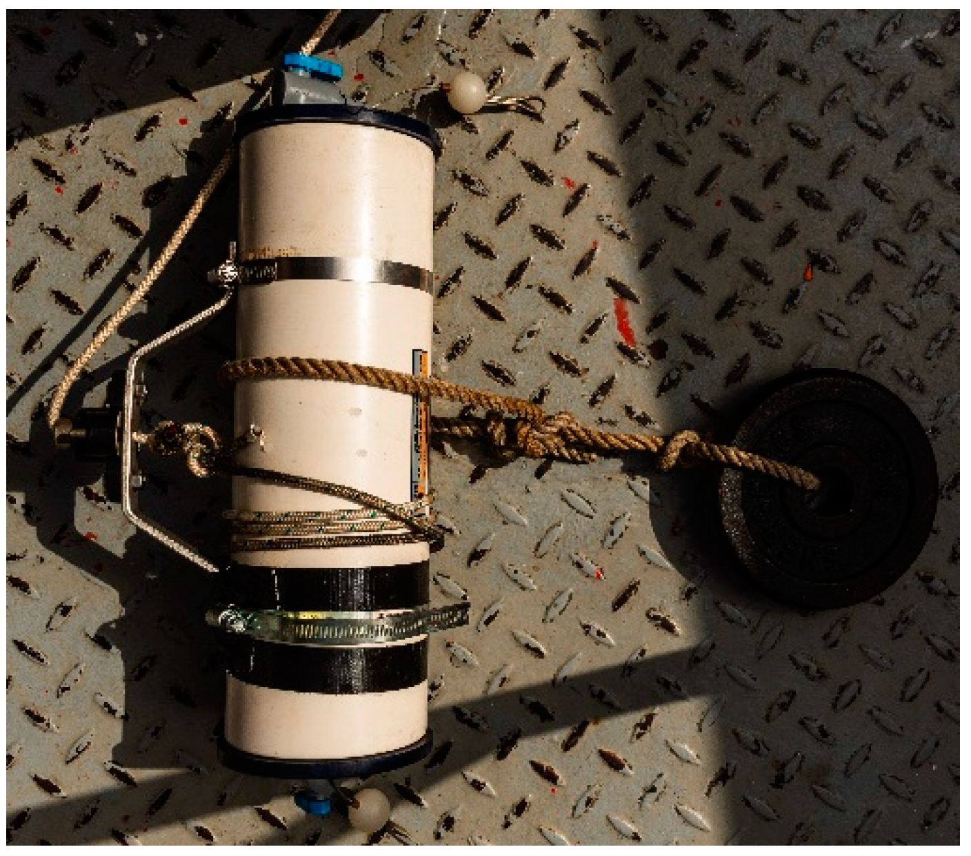
2.3. Cartridge Filtration

Cartridge filtration was performed 200 m downstream of the depth sample location, where anchoring was possible (Circle Figure 1B). The sampling took place from a boat anchored to the southern side of the main current. A hose was extended into the water to a depth of approximately 10 cm, connected to a 12 V water pump, which fed into the filtration unit. To prohibit large debris from entering the pump, a mesh basket with a pore size of 5 mm was attached to the end of the hose. Filtration took place until the filter was clogged and the water flow through the filter stopped completely. The amount of water filtered was measured with an in-line water volume meter (GARDENA).
The used cartridge filters were provided by Wolftechnik and were equipped with a 10 µm stainless steel filter element. Five filtration samples were taken.
To store the samples, each cartridge with the filter element and the remaining water inside was sealed and stored at room temperature until sample preparation.

2.4. Net Filtration

The sample location for the net filtration was the same as for the cartridge filtration.
Two plankton nets with pore sizes of 65 µm and 105 µm were used. The nets were fixed to the end of a pole to provide further reach. During sampling, the nets were held fully submerged below the water line.
To determine the amount of water filtered, the current was measured before filtration with the ‘Rod Held Current Meter RHCM 3 × 90 cm’ by HYDRO-BIOS. For the measurement, the current speeds of six ten-second intervals were averaged. A volume of 1000 L was filtered. To filter this volume, the time of filter submersion had to be calculated (Equation (1)).
t = v c u r r e n t · 10 6 c m 3 A n e t
t , Time the net had to be in the water to filter 1000 L
v c u r r e n t , Speed of the current
A n e t , Circular area of the net.
After the sample was taken, nets were rinsed from the outside to transfer all of the particles stuck to the net into the sampling flask at the end of the net. The samples were then stored in the flask for further analysis.

2.5. Time of Sampling

All of the Samples were taken on the same day. First, depth samples were taken. The time in between the depth samples was approximately 10 min. After the depth samples, the net filtration was started with a 3 h break in between. Each net filtration took about 15 min of preparation, resulting in a 20 min interval. The cartridge filtration was started right after the last net filtration, with each round taking approximately 30 min.

2.6. Sample Preparation

All samples were prepared the same way.
Alkaline digestion was chosen to reduce biofilms on polymer particles and other organic materials. This was combined with density separation.
For the organic digestion, the samples were treated in 5 molar NaOH (ROTH) for 7 days. The samples were then filtered onto a stainless-steel mesh filter with 10 µm pores to separate the particles from the alkaline solution. For density separation, the samples were then transferred from the stainless-steel filter to 100 mL ZnCl2 solution. This was performed by treating the loaded filter for 3 min in an ultrasonic bath (Heraeus minison 150/300). The ZnCl2 (SIGMA-ALDRICH) solution was prepared with a density of 1.6 g∙mL−1. The sample suspension was then transferred into separation funnels and left to settle for 7 days. Afterward, about 80% of the suspension was discarded, and the remaining liquid was strained through a 10 µm stainless-steel filter and washed with 1 molar HCL solution to remove all ZnCl2, including the ZnCl2 precipitate. The residue on the stainless-steel filter was then resuspended into 100 mL deionized water by 3 min treatment in the ultrasonic bath. The resulting water-particle suspension was filtered through a 0.2 µm aluminum oxide filter (Whatman Anodisc).
The aluminum oxide filters were then stored in separate petri dishes for analysis.
Throughout the process, an attempt was made to minimize factors of possible further contamination with microplastics by using glassware, only wearing cotton clothing, and reducing the times that samples were opened, as well as working under a fume hood. It was not possible to do the preparation procedures in a cleanroom, and not all solutions could be filtered before use. Therefore, multiple control samples were prepared in parallel.

2.7. Analytic Methods

The analysis of the microplastic particles was performed by FT-IR spectrometry (Spotlight 200i FT-IR Microscopy System and Spectrum V10.6.2 software by PerkinElmer). Three squares of each filter were chosen, on which all particles with a size of at least 20 µm were analyzed with the single-point detector. To eliminate operator bias, the squares were set at specific coordinates on the filter (Figure 3). The squares analyzed on the filter had a size of 250 × 250 µm, resulting in an area of 62,500 µm2. The diameter of the filter equaled 18,820 µm, resulting in a filter area of 278,182,060.4 µm2. The spectra were then compared in the spectrometer software with a polymer spectrum database. All hits with a correlation of over 70% were counted. The data were then extrapolated to the full area of the filter.
From the acquired data of each filter, the data from the control samples was subtracted, and the particle amount per liter was calculated.
The significance of the variation between the different data sets was tested using two-sample t-tests.
The average density of each of the three depth samples per depth was calculated as seen in Equation (2). The densities used can be seen in Table 1.
In the case of some polymers, multiple different variations with different densities exist. In these cases, the density of the least dense polymer variation was chosen. All calculations performed regarding densities in this paper refer to the minimum density.
  ρ p l a s t i c   p a r t i c l e s a m p l e = N p l a s t i c   p a r t i c l e ρ p l a s t i c   p a r t i c l e N g l o b a l   p l a s t i c   p a r t i c l e
ρ p l a s t i c   p a r t i c l e s a m p l e , Average density of all polymers per depth sample
ρ p l a s t i c   p a r t i c l e , Density of the polymer in question
N p l a s t i c   p a r t i c l e , Number of particles of the polymer in question
N g l o b a l   p l a s t i c   p a r t i c l e , Number of particles of all polymers in the sample

2.8. Method Comparison

Different methods were compared by the amount of polymer particles larger than 20 µm found. The methods that were compared are net filtration with pore sizes 65 µm and 105 µm, cartridge filtration, and the depth samples combined and only the sample just below the surface (Table 2). In this comparison, only the microplastic particle amount was considered. The polymer type was not taken into account.

3. Results

Microplastic particles were found in all analyzed samples of the Danube delta. In one liter of water, 46 microplastic particles with a size larger than 105 µm (CV [coefficient of variation] = 62%), 95 particles larger than 65 µm (CV = 53%), and 2677 microplastic particles larger than 20 µm (CV = 11%) were found (Further information: Table 3). On the day of sampling, the discharge of the Danube, as measured at the hydrological station in Isaacea, was 4190 m3∙s−1. With the assumption that the microplastic load does not change with higher or lower discharge and an annual average discharge of 6416 m3∙s−1 [33], this adds up to approximately 1.72 × 10¹⁰ microplastic particles per second (>20 µm). This number has been calculated using the results of the cartridge filtration since this method had the smallest coefficient of variation.

3.1. Polymer Composition in the Water Column

To analyze the polymer composition throughout the water column, samples were taken close to the surface of the river and at depths of 3 m and 6 m. The results of all depths combined show that 46% of all polymers found are polyethylene terephthalate (PET). This is followed by polytetrafluorethylene (PTFE) with 24% and polyethylene (PE) with 11%.
In all depth samples, PET had the highest quantity, with 63% close to the surface, 30% at 3 m, and 55% at 6 m. The second highest amount of polymer particles was PTFE, with 23% at 0 m and 55% at 6 m, whereas at 3 m, PTFE only had a percentage of 18%. At 3 m depth, PE showed 22%, a larger percentage than PTFE. Close to the surface, PE also had a larger fraction with 6%, but at 6 m, it made up a minor portion with less than one percent. Polycarbonate (PC) showed a larger percentage, with seven percent at 6 m. At 3 m, further large portions were polyamide (PA) with 11% and ethylenevinyl acetate (EVA) with 10% (Figure 4A).

3.2. Polymer Density in the Water Column

The average density of all depth samples was calculated to quantify the different polymer compositions in correlation to their density (Equation (2)). At 0 m, the average density was calculated to be 1.42 g∙cm−3, 1.44 g∙cm−3 at 3 m, and 1.64 g∙cm−3 at 6 m. The difference in densities was not found to be significant, with standard deviations of 0.20 g∙cm−3 in the 0 m samples, 0.04 g∙cm−3 in the 3 m, and 0.22 g∙cm−3 in the 6 m samples (Figure 4B).

3.3. Polymer Particles in the Water Column

The number of polymer particles found in the three sampled depths showed no significant difference. An average of 31,706 p∙L−1 (microplastic particles per liter) with a size over 20 µm were found at the surface of the river. At 3 m depth, 62,882 p∙L−1 and at 6 m depth, 58,114 p∙L−1 were found. The coefficient of variation amounts to 37% at 0 m, 30% at 3 m, and 155% at 6 m (Figure 4C).

3.4. Polymer Composition in Cartridge and Net Filtrations

Furthermore, the polymer composition of the cartridge filtration and the two net filtration values were determined (Figure 4A; Table 4). As in the depth samples, PET was the most abundant polymer, followed by PTFE in the cartridge filtration and by Ethylene Vinylalcohol Copolymer (EVOH) in both of the net filtrations. The percentages of the findings are 66% PET, 28% PTFE, 2% EVOH, and 1% PPT in the cartridge filtration samples. The 105 µm net samples yielded percentages of 37% PET, 31% EVOH, 12% PA, 10% PE, 6% PTFE, and 3% PBT. Filtration with the 65 µm nets yielded percentages of 30% PET, 38% EVOH, 11% PTFE, 10% EVA, 8% PE, 7% PA, 4% PBT, and 2% PU.

3.5. Method Comparison

For method comparison, net filtration (65 µm; 105 µm), cartridge filtration, and the depth samples (average of 0 m, 3 m, 6 m; only 0 m) were compared. Since sample preparation and analysis were performed the same way in all samples, the particle size detection limit was 20 µm for all methods. Net filtration with a mesh of 105 µm pores yielded an average number of 46 p∙L−1. In nets with 65 µm pores, an average of 95 p∙L−1 was found. The coefficient of variation was calculated to be 62% in the 105 µm net samples and 53% in the 65 µm net samples. The cartridge filtration gave an average particle count of 2677 p∙L−1 with a coefficient of variation of 11%. By combining all the depth samples, an average of 37,007 p∙L−1 with a variation coefficient of 72% was found. An outlier in the 6 m depth sample was not included in this calculation. By only taking the 0 m samples of the depth sample experiment, 31,706 p∙L−1 could be identified with a coefficient of variation of 37% (Table 3).
With this data, significant differences were found between the cartridge filtration and both of the two net filtrations. Both the 0 m depth sample and all depth samples evaluated together also show significant differences between the two net filtrations and the cartridge filtration (Figure 5).

4. Discussion

4.1. Depth Samples

The results of the depth samples show no significant difference in the number of particles found in different water depths (Figure 4C). This is contrary to what the data shown by Liedermann et al. [5] suggests. The study was performed in Austria, and the particle amounts close to the Danube River floor were lower than the amounts further up in the water column. The difference could be rooted in the fact that Liedermann et al. used bridges as sampling stations, whereas the depth samples of this paper were taken from a moving ship. While water can flow relatively undisturbed under a bridge, the ship propellors might have introduced turbulences reaching through the water column. Another reason could be the difference in particle sizes analyzed.
A significant increase in particle density with increasing water depth was not found in this study (Figure 4B). Similar results were found by Lenaker et al. [17]. Their study was performed in the Milwaukee River Basin. 333 µm nets were used in all depths, and a correlation between depth and microplastic particle density could not be shown significantly. Taking both findings, a hypothesis that smaller particles do not have a more homogenous distribution throughout the water column can be presented. This needs further investigation since the depth sample findings of our study could have been heavily influenced by the following circumstances. Besides a small sample size of the depth samples, other factors include the unusually strong trafficked Danube by large ships due to harbor closures along the Ukrainian coast and the fact that the depth samples were taken from a moving ship. These may have led to increased turbulence and mixing of the river by ship propellors. Another suggested reason for inaccuracies of observed microplastic distribution in the water column is biofouling and biofilm, which may lead to a density increase of microplastic particles [34].
Most studies have found PA, PE, PET, PP, and PVC to be the most abundant microplastics throughout the water column [17,18,35]. This mostly correlates with the results of this study, with the exception of PTFE (Figure 4A). The polymer was also detected by Pojar et al. [14] in sediment samples of the Danube River delta and coast region but only constituted 4% of the microplastics found. The reason for the enormous amounts found in this study is unknown. In general, a possible source for PTFE is the producing industry, which is often located close to large water sources like the Danube. Due to its high heat resistance and its non-stick properties, PTFE is often used in high-temperature environments and in coatings [4]. The actual values of PTFE particles in the water are presumed to be even larger since a portion was most likely separated during density separation (density of PTFE: 2.12 g∙cm−3; density separation with ZnCl2: 1.6 g∙mL−1).

4.2. Method Comparison: Particle Composition

The different mesh sizes of filtration used in this study were 10 µm using cartridge filtration (detection limit: 20 µm) and 65 µm and 105 µm using net filtration. As seen in Figure 4A and Table 4, the polymer distribution of the 20 µm fraction (PET > PTFE > EVOH > PPT > …) differs from the polymer distribution of the 65 µm (PET > EVOH > PTFE > EVA > …) and 105 µm (PET > EVOH > PA > PE > …) fractions. Taking into account that most microplastic found in this study was deemed secondary microplastic (Supplementary Data Figure S1), this either suggests that some polymers break down more easily than others or that the detected smaller microplastic particles entered the river further upstream and were exposed to UV radiation and physical forces for a longer period of time. Another possibility is that the sources of larger microplastics differ from the sources of smaller microplastics. Either way, it shows that sampling methods with different size characteristics cannot be compared. This is especially true when comparing different methods, as performed here with cartridge and net filtration.

4.3. Method Comparison: Particle Amount

The conclusion that different methods cannot be compared can also be drawn from the particle amounts detected by the different mesh sizes. With 46 p∙L−1 at 105 µm, 95 p∙L−1 at 65 µm and 2677 p∙L−1 at 10 µm (detection limit: 20 µm), a negative logarithmic correlation between mesh size and particle amount is therefore possible. This assumption needs further investigation with a larger sample size and with more similar filtration methods.
Other studies have also found that smaller microplastic particles are more abundant in rivers than larger ones. Dris et al. [36] saw a 100-fold increase in numbers during comparison of an 80 µm plankton net and a 330 µm manta trawl.
The overall amount of microplastics found in this study is greater than that found in existing literature. Studies mostly report numbers between 0.0005 p∙L−1 and 16 p∙L−1 [4]. Whether these disparities arise from the geographical and anthropogenic differences between the sample locations or the different mesh sizes used during sampling is not known.
When comparing the numbers of the net and cartridge filtration with the numbers generated by depth sampling, the differences shown are even larger (Figure 5). With 31,706 p∙L−1 at 0 m, 62,882 p∙L−1 at 3 m, and 58,114 p∙L−1 at 6 m, the particle load is between 11-fold and 23-fold higher than the load measured by cartridge filtration. The reason for this difference is unknown. Depth samples at 0 m and cartridge filtration should, in theory, show similar data because of the same 20 µm particle cutoff size during analysis. The difference cannot be clearly attributed to mistakes in sample preparation or sample analysis since all samples were treated the same during these steps. The high variance shown by the depth samples can be explained by the small sample size. Due to the higher sample volume and the smaller variance, we believe that the microplastic particle numbers obtained by cartridge filtration are more accurate. This is also the reason why the data received by cartridge filtration was used for the calculation of the annual particle load of the Danube.
Nonetheless, the numbers shown in this study are still likely to be below the actual number of plastic particles in the river. The detection limit of particles in this paper was 20 µm. Therefore, the amounts shown likely underestimate the true values.

5. Conclusions

The data collected in this study shows a large amount of microplastics in the surface water of the Danube River delta. 2677 p∙L−1 is the highest ever reported concentration of microplastic particles (>20 µm in size; analyzed using cartridge/pump filtration) in the Danube. The results of the different filtration methods used for sampling suggest a negative logarithmic correlation between mesh size and detected numbers of microplastic particles.
The different quantities, as well as the different polymer compositions of the filtration methods, clearly show that it is not possible to compare studies that use dissimilar methodologies. It is therefore necessary to either investigate the correlation between mesh sizes and detected microplastics and, therefore, to allow extrapolation or to standardize sampling methods. Furthermore, a trend to standardize 300 µm nets, as currently undertaken, is shown to highly underestimate the actual amounts of microplastics in the water. We suggest not to only use one mesh size while sampling but to include a variety of sizes.
A significant change in microplastic distribution and density throughout the water column could not be shown.
In conclusion, our study reveals an alarming presence of microplastics in the Danube River delta, emphasizing the need for standardized sampling methods and a deeper exploration of microplastic behavior at various depths within fluvial systems. We greatly appreciate the opportunity to contribute to this critical field of research and look forward to advancing our collective understanding of microplastic pollution in aquatic environments.

Supplementary Materials

The following supporting information can be downloaded at https://www.mdpi.com/article/10.3390/microplastics2040025/s1, Figure S1: Principle of single spot particle analysis in the PerkinElmer FT-IR Microscopy System. (A) Operator view of the 500 µm × 500 µm microscope image with marked particles. Each red and white dashed square (20 µm × 20 µm) equals one marked particle. All unmarked particles did not fit the criteria or were out of bound. (B) same view as ‘A’ without the markings; Figure S2: (A) Example spectra of Polyethylene (PE) with a correlation coefficient of 0.79. (B) Example spectra of Polyamide (PA) with a correlation coefficient of 0.70. A Correlation of 70 % was chosen to be the smallest correlation counted as positive; Table S1: Polymer composition calculated by summation of particle numbers of samples of each sampling method; Table S2: Particle numbers of each sample of the sampling methods.

Author Contributions

Conceptualization, A.F. and T.K.; analysis and writing—original draft preparation, T.K.; writing—review and editing, T.K. and M.K. All authors have read and agreed to the published version of the manuscript.

Funding

This research received no external funding.

Institutional Review Board Statement

The study did not require ethical approval.

Informed Consent Statement

The study did not involve humans.

Data Availability Statement

Data Availability is available in Supplementary Materials.

Acknowledgments

Every support given is covered by the author’s contribution.

Conflicts of Interest

The authors of this paper declare that they have no personal relationships or competing financial interest that could have influenced the work reported in this paper.

References

  1. Johansen, M.R.; Christensen, T.B.; Ramos, T.M.; Syberg, K. A review of the plastic value chain from a circular economy perspective. J. Environ. Manag. 2022, 302, 113975. [Google Scholar] [CrossRef] [PubMed]
  2. Plastics Division: Life Cycle of a Plastic Product. Available online: https://web.archive.org/web/20100317004747/http://www.americanchemistry.com/s_plastics/doc.asp?CID=1571&DID=5972 (accessed on 7 December 2022).
  3. Jambeck, J.R.; Geyer, R.; Wilcox, C.; Siegler, T.R.; Perryman, M.; Andrady, A.; Narayan, R.; Law, K.L. Plastic waste inputs from land into the ocean. Science 2015, 347, 768–771. [Google Scholar] [CrossRef] [PubMed]
  4. Horton, A.A.; Walton, A.; Spurgeon, D.J.; Lahive, E.; Svendsen, C. Microplastics in freshwater and terrestrial environments: Evaluating the current understanding to identify the knowledge gaps and future research priorities. Sci. Total Environ. 2017, 586, 127–141. [Google Scholar] [CrossRef] [PubMed]
  5. Liedermann, M.; Gmeiner, P.; Pessenlehner, S.; Haimann, M.; Hohenblum, P.; Habersack, H. A Methodology for Measuring Microplastic Transport in Large or Medium Rivers. Water 2018, 10, 414. [Google Scholar] [CrossRef]
  6. Zhang, S.; Wang, J.; Liu, X.; Qu, F.; Wang, X.; Wang, X.; Li, Y.; Sun, Y. Microplastics in the environment: A review of analytical methods, distribution, and biological effects. TrAC Trends Anal. Chem. 2019, 111, 62–72. [Google Scholar] [CrossRef]
  7. Galgani, F.; Hanke, G.; Werner, S.; De Vrees, L. Marine litter within the European Marine Strategy Framework Directive. ICES J. Mar. Sci. 2013, 70, 1055–1064. [Google Scholar] [CrossRef]
  8. Streit-Bianchi, M.; Cimadevila, M.; Trettnak, W. Mare Plasticum—The Plastic Sea Combatting Plastic Pollution through Science and Art; Springer: Cham, Switzerland, 2020. [Google Scholar]
  9. Lechner, A.; Ramler, D. The discharge of certain amounts of industrial microplastic from a production plant into the River Danube is permitted by the Austrian legislation. Environ. Pollut. 2015, 200, 159–160. [Google Scholar] [CrossRef] [PubMed]
  10. Wagner, M.; Lambert, S. Freshwater Microplastics the Handbook of Environmental Chemistry 58 Series Editors: Damià Barceló · Andrey G. Kostianoy. Available online: http://www.springer.com/series/698 (accessed on 9 December 2022).
  11. Stock, F.; Kochleus, C.; Bänsch-Baltruschat, B.; Brennholt, N.; Reifferscheid, G. Sampling techniques and preparation methods for microplastic analyses in the aquatic environment—A review. TrAC Trends Anal. Chem. 2019, 113, 84–92. [Google Scholar] [CrossRef]
  12. Lechner, A.; Keckeis, H.; Lumesberger-Loisl, F.; Zens, B.; Krusch, R.; Tritthart, M.; Glas, M.; Schludermann, E. The Danube so colourful: A potpourri of plastic litter outnumbers fish larvae in Europe’s second largest river. Environ. Pollut. 2014, 188, 177–181. [Google Scholar] [CrossRef] [PubMed]
  13. Kittner, M.; Kerndorff, A.; Ricking, M.; Bednarz, M.; Obermaier, N.; Lukas, M.; Asenova, M.; Bordós, G.; Eisentraut, P.; Hohenblum, P.; et al. Microplastics in the Danube River Basin: A First Comprehensive Screening with a Harmonized Analytical Approach. ACS ES&T Water 2022, 2, 1174–1181. [Google Scholar] [CrossRef]
  14. Pojar, I.; Stănică, A.; Stock, F.; Kochleus, C.; Schultz, M.; Bradley, C. Sedimentary microplastic concentrations from the Romanian Danube River to the Black Sea. Sci. Rep. 2021, 11, 2000. [Google Scholar] [CrossRef] [PubMed]
  15. Pojar, I.; Tirondutu, L.; Pop, C.I.; Dutu, F. Hydrodynamic Observations on Microplastic Abundances and Morphologies in the Danube Delta, Romania. AgroLife Sci. J. 2021, 10, 142–149. [Google Scholar] [CrossRef]
  16. Miklós, D.; Neppel, F. Palaeogeography of the Danube and Its Catchment. In Hydrological Processes of the Danube River Basin; Springer: Dordrecht, The Netherlands, 2010; pp. 79–124. [Google Scholar] [CrossRef]
  17. Lenaker, P.L.; Baldwin, A.K.; Corsi, S.R.; Mason, S.A.; Reneau, P.C.; Scott, J.W. Vertical Distribution of Microplastics in the Water Column and Surficial Sediment from the Milwaukee River Basin to Lake Michigan. Environ. Sci. Technol. 2019, 53, 12227–12237. [Google Scholar] [CrossRef] [PubMed]
  18. Liu, K.; Courtene-Jones, W.; Wang, X.; Song, Z.; Wei, N.; Li, D. Elucidating the vertical transport of microplastics in the water column: A review of sampling methodologies and distributions. Water Res. 2020, 186, 116403. [Google Scholar] [CrossRef] [PubMed]
  19. Park, T.-J.; Lee, S.-H.; Lee, M.-S.; Lee, J.-K.; Lee, S.-H.; Zoh, K.-D. Occurrence of microplastics in the Han River and riverine fish in South Korea. Sci. Total Environ. 2020, 708, 134535. [Google Scholar] [CrossRef] [PubMed]
  20. Tockner, K.; Uehlinger, U.; Robinson, C.T. Rivers of Europe; Academic Press: Cambridge, MA, USA, 2009; Available online: https://books.google.de/books?hl=de&lr=&id=GDmX5XKkQCcC&oi=fnd&pg=PT75&dq=danube+drainage+basin&ots=CTZeJ4zYUU&sig=DZ1-KTx9A8OkgZ14HLVt0ikZ1Jw&redir_esc=y#v=onepage&q&f=false (accessed on 28 September 2023).
  21. Schiemer, F.; Guti, G.; Keckeis, H.; Staras, M. Ecological Status and Problems of the Danube River and Its Fish Fauna: A Review. Available online: https://www.researchgate.net/publication/290485507_Ecological_status_and_problems_of_the_Danube_River_and_its_fish_fauna_a_review (accessed on 16 January 2023).
  22. Polycarbonate|Density, Strength, Melting Point, Thermal Conductivity. Available online: https://material-properties.org/polycarbonate-density-strength-melting-point-thermal-conductivity/ (accessed on 6 December 2022).
  23. Ethylene -Propylene-Diene Rubber- EPDM with Density 0.87 g/cm3—Indian Products Directory. Available online: https://suppliers.jimtrade.com/81/80508/ethylene_propylenediene_rubber_epdm_with_density_0_87_g_cm3.htm (accessed on 6 December 2022).
  24. LDPE. Available online: https://www.polymerdatabase.com/Commercial%20Polymers/LDPE.html (accessed on 6 December 2022).
  25. Poly(ethersulfone). Available online: https://polymerdatabase.com/polymers/polyethersulfone.html (accessed on 6 December 2022).
  26. Poly(ethylene Terephthalate). Available online: https://www.polymerdatabase.com/polymers/polyethyleneterephthalate.html (accessed on 6 December 2022).
  27. Poly(tetrafluoroethylene). Available online: https://www.polymerdatabase.com/polymers/polytetrafluoroethylene.html (accessed on 6 December 2022).
  28. ‘AKROMID® S3 1 Natural (3484)’, Poly-Amide 6.10. Available online: https://akro-plastic.com/productfilter/details/3484/ (accessed on 6 December 2022).
  29. Polybutylene Terephthalate (PBT)—Properties and Applications—Supplier Data by Goodfellow. Available online: https://www.azom.com/article.aspx?ArticleID=1998 (accessed on 6 December 2022).
  30. Erwin Telle. Polysulfon. Available online: https://www.telle.de/en/production-products/plastics/material-range/product/detail/polysulfone-psu/ (accessed on 6 December 2022).
  31. McKeen, L.W. Film Properties of Plastics and Elastomers; Elsevier: Amsterdam, The Netherlands, 2012. [Google Scholar] [CrossRef]
  32. Density of Plastics, Density of PVC. Available online: https://polymeracademy.com/density-of-various-plastic/ (accessed on 6 December 2022).
  33. Pekárová, P.; Miklánek, P. Flood Regime of Rivers in the Danube River Basin; Ústav Hydrológie SAV: Bratislava, Slovakia, 2019. [Google Scholar] [CrossRef]
  34. Kooi, M.; van Nes, E.H.; Scheffer, M.; Koelmans, A.A. Ups and Downs in the Ocean: Effects of Biofouling on Vertical Transport of Microplastics. Environ. Sci. Technol. 2017, 51, 7963–7971. [Google Scholar] [CrossRef] [PubMed]
  35. Choy, C.A.; Robison, B.H.; Gagne, T.O.; Erwin, B.; Firl, E.; Halden, R.U.; Hamilton, J.A.; Katija, K.; Lisin, S.E.; Rolsky, C.; et al. The vertical distribution and biological transport of marine microplastics across the epipelagic and mesopelagic water column. Sci. Rep. 2019, 9, 7843. [Google Scholar] [CrossRef] [PubMed]
  36. Dris, R.; Gasperi, J.; Rocher, V.; Saad, M.; Renault, N.; Tassin, B. Microplastic contamination in an urban area: A case study in Greater Paris. Environ. Chem. 2015, 12, 592–599. [Google Scholar] [CrossRef]
Figure 1. Sampling sites and depths (marked in red) (A) sample location on the Danube: before the Danube delta, between Romania and Ukraine; (B) geographic features of the Danube in the sample area; (C) topographic features of the sample area; (D) sample depths. Maps from danubegis.org and navionics.com (accessed on 28 October 2022).
Microplastics 02 00025 g001
Figure 2. 2.2 L sampling tube from WILDCO with added weight for faster sinking.
Microplastics 02 00025 g002
Figure 3. (A) Filter with marked analysis square locations (); (B): loaded aluminum oxide filter.
Microplastics 02 00025 g003
Figure 4. (A) Polymer composition of the depth samples at 0 m, 3 m, and 6 m of the cartridge filtration and the two net filtrations (65 µm; 105 µm). (B) Average density of polymer particles found in the three different depths (ns: no significant difference); (C) Comparison of depth samples by number of plastic particles found (ns: no significant difference; -: average value).
Microplastics 02 00025 g004
Figure 5. Comparison of sampling methods by number of plastic particles found (only significant differences shown). Microplastics 02 00025 i001: sample value; ▪: calculated average value; Microplastics 02 00025 i002
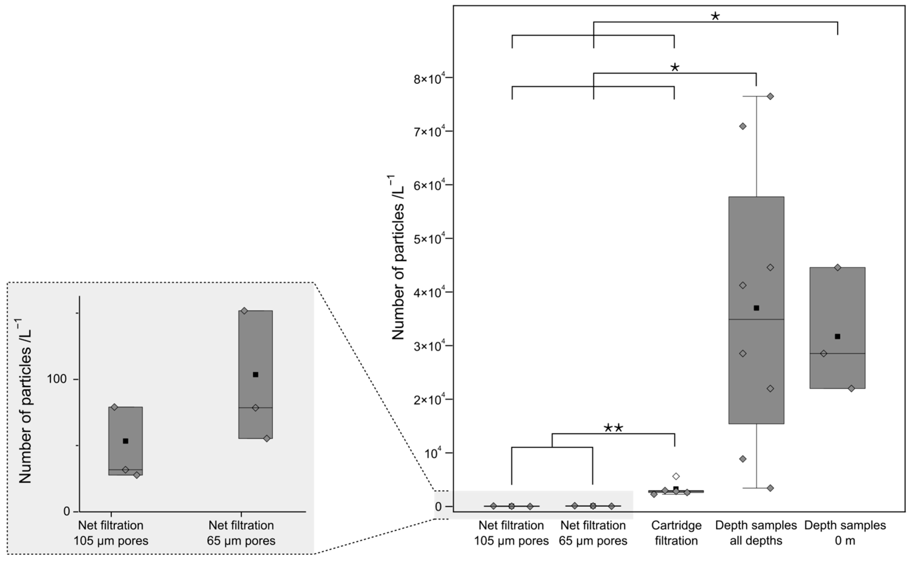
: outlier; *: significant difference of p < 0.05; **: significant difference of p < 0.01. Each box shows the interquartile range with the middle line showing the median. The whiskers depict the minimum and maximum for datasets with more than three values. Values of more than 1.5 times the interquartile range were deemed outliers and were not used in the evaluation but are still shown.
Microplastics 02 00025 g005
Table 1. The densities of the polymers are used to calculate the average density [22,23,24,25,26,27,28,29,30,31,32].
PolymerDensity/g∙cm−3
Ethylene Vinylalcohol Copolymer (EVOH)1.9
Ethylenevinyl acetate (EVA)0.95
Polyamid (PA)1.01
Polybutylene terephthalate (PBT)1.31
Polyethylene terephtalate (PET)1.34
Polysulfone (PSU)1.42
Polytetrafluorethylene (PTFE)2.12
Polycarbonate (PC)1.2
Polyether sulfone (PES)1.37
Polypropylene terephthalate (PPT)1.31
Polyethylene (PE)0.9
Polypropylene (PP)0.861
Table 2. Methods and method subdivisions used for the method comparison based on polymer particle amount.
Filtration MethodMethod Subdivision
Net FiltrationNet with pore size: 65 µm
Net FiltrationNet with pore size: 105 µm
Cartridge Filtration
Depth Samplesparticle numbers of all depths (0 m, 3 m, 6 m) averaged
Depth Samplesparticle numbers of 0 m
Table 3. Resulting in polymer particle numbers of the respecting filtration methods, including their calculated coefficient of variation.
Filtration MethodMethod SubdivisionParticle CountCV
Net Filtration65 µm95 p∙L−153%
Net Filtration105 µm46 p∙L−162%
Cartridge Filtration 2677 p∙L−111%
Depth Samplesall depths averaged50,901 p∙L−172%
Depth Samples0 m31,706 p∙L−137%
Table 4. Most abundant polymers per liter from cartridge and net filtrations. Sorted after the most abundant polymer.
Cartridge FiltrationNet Filtration (65 µm)Net Filtration (105 µm)
Polymerp∙L−1Polymerp∙L−1Polymerp∙L−1
PET1378PET28PET17
PTFE575EVOH27EVOH14
EVOH51PTFE10PE5
PPT37EVA9Nylon5
PVC25PE7PTFE3
Disclaimer/Publisher’s Note: The statements, opinions and data contained in all publications are solely those of the individual author(s) and contributor(s) and not of MDPI and/or the editor(s). MDPI and/or the editor(s) disclaim responsibility for any injury to people or property resulting from any ideas, methods, instructions or products referred to in the content.

