
Accuracy of a Simple Microplastics Investigation Method on Sandy Beaches


Institute of Integrated Sciences and Technology, Nagasaki University, Nagasaki 852-8521, Japan
Microplastics 2023, 2(3), 304-321; https://doi.org/10.3390/microplastics2030024
Submission received: 19 June 2023
/
Revised: 9 August 2023
/
Accepted: 14 September 2023
/
Published: 17 September 2023
Abstract
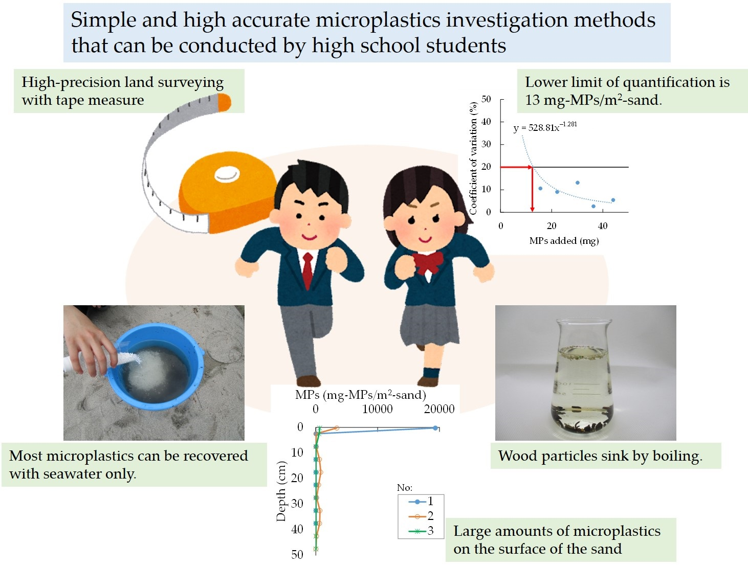
:Environmental pollution by microplastics (MPs) has become a growing concern, and not only professional researchers but also the citizenry are needed to understand the pollution situation and to confirm the decreasing trend of MP pollution as a result of the global reduction in plastic use. In this study, the author evaluated the accuracy of a simple method of investigating MPs on sandy beaches that can be conducted even by high school students. In a land survey using simple tools such as a tape measure and cardboard, the maximum coefficient of variation is approximately 1%. Even without heavy liquid, 89% of MPs could be recovered using only seawater. An investigation of MP content by sampling 0.5 cm of the surface layer of sand could explain more than half of the MP content when the sand was sampled to a depth of approximately 50 cm below the surface layer. A method in which the recovered MPs are not visually sorted but floating matter after boiling is considered as MPs is acceptable. If there was no concern about pumice contamination, the overestimation was approximately 1.5 times. Simple laboratory equipment such as buckets, sieves, seawater, hot plates, dryers, and electronic balances could achieve lower limits of quantification of MPs of 13 mg-MPs/m2-sand and 2 mg-MPs/kg-sand.

1. Introduction
Plastics have become an indispensable material in people’s lives owing to their light weight and durability, and their continuous and massive production has led to the global pollution of the environment with plastic waste [1]. Between 4 and 12 million metric tons of land-based plastic waste is estimated to have entered the marine environment in 2010 alone [2], and the forecast is for a cumulative increase to 12 billion metric tons by the year 2050 [3]. Common plastics accumulate in landfills and the natural environment because they decompose very slowly under natural conditions [4]. This is why the almost permanent pollution of the natural environment by plastic waste is becoming more and more of a problem. Meanwhile, plastic debris breaks down into small fragments called microplastics (MPs) under the UV rays of sunlight mechanical abrasion [5,6], and MPs have been detected in major oceans and coastal areas [4]. Cole et al. (2011) have found that MPs make up a significant portion of the marine litter in the ocean [7].
MPs may accumulate organic contaminants such as carcinogenic polychlorinated biphenyls (PCBs) [8,9,10], polycyclic aromatic hydrocarbons (PAHs), heavy metals, and others [11,12], which eventually leads to organic pollutants entering the marine food web through ingestion and accumulation by zooplankton, bivalves, and fish [13]. Plastics were detected in the gastrointestinal tracts of 36.5% of fish in the English Channel [14]. Plastic fragments detected in the stomachs and abdominal fat of oceanic seabirds have been found to contain polybrominated diphenyl ethers [15].
In an effort to address the complex challenges facing our planet, the United Nations General Assembly adopted 17 Sustainable Development Goals (SDGs) in September 2015. Sustainable Development Goal 14 (SDG 14) aims to “conserve and sustainably use the oceans, seas, and marine resources for sustainable development”. Goal 14.1 of SDG 14 is the prevention and significant reduction of marine pollution of all kinds. The density of plastic debris (14.1.1b) is an indicator of marine pollution. The publication of “A European Strategy for Plastics in a Circular Economy” in January 2018 by the European Union (EU) was followed by the setting of new recycling targets and the proposal of regulations for single-use plastics (DIRECTIVE OF THE EUROPEAN PARLIAMENT AND OF THE COUNCIL on the reduction of the impact of certain plastic products on the environment) in May 2018. This will help prevent marine pollution and reduce the use of plastics around the world. The amount of MPs in the environment is likely to decrease over the long term as these measures take effect, although there may be a need for the collection of plastic waste which is present.
MPs have been extensively studied in marine sediments such as sand [9,16,17,18,19,20,21,22,23,24,25,26]. However, those studies use various approaches to identify, quantify, and report measured concentrations of MPs, making spatiotemporal comparisons difficult [27].
Attempts have been made to standardize the investigation method for beach litter. United Nations Environment Programme (UNEP) Guidelines [28], Oslo Paris (OSPAR) Commission [29], and National Oceanic and Atmospheric Administration (NOAA) [30] have introduced investigation methods for coastal marine litter. Although these methods target not only MPs but mainly large marine litter, the methods for determining study sites and recording data can be used as a reference. The Marine Directors of the EU, acceding countries, candidate countries, and European Free Trade Association countries have jointly developed a common strategy for supporting the implementation of Directive 2008/56/EC, the “Marine Strategy Framework Directive” (MSFD). In order to achieve or maintain Good Environmental Status (GES) in European seas, the “Guidance on Monitoring of Marine Litter in European Seas” has been developed (Joint Research Centre Scientific and Policy Reports, JRC) [31]. The GESAMP Working Group (WG40) on “Sources, fate, and effects of plastics and microplastics in the marine environment”, co-led by the Intergovernmental Commission on Oceanography (IOC-UNESCO) and the UNEP, has issued a report “Guidelines for the Monitoring and Assessment of Plastic Litter in the Ocean” (Group of Experts on the Scientific Aspects of Marine Environmental Protection, GESAMP) [32]. The principal purpose of the report is to provide recommendations, advice, and practical guidance for establishing programs to monitor and assess the distribution and abundance of plastic litter in the ocean. The JRC and GESAMP protocols provide methods for investigating microplastics.
Suppose we want to test the hypothesis that, in the long run, MPs will decrease as plastics are used less. In this case, we need to develop a simple method of investigation that can be carried out by the citizens and can increase the rate of data accumulation of the MPs, instead of relying on costly professional research. JRC (2013) states that investigation by volunteers including the citizenry lowers costs, serves as an early warning system, and generates more data series [31]. GESAMP (2019) states that citizen scientists represent a very important resource for gathering information on the environment [32].
The above guidelines have introduced an investigation method that can be conducted by the citizenry. The author is committed to the development of a simple method for investigating MPs on sandy beaches that can be performed by high school students. The Japanese Ministry of Education, Culture, Sports, Science and Technology (MEXT) has recommended that students, including high school students, engage in exploratory activities. In this regard, MP research activities are a prime opportunity for students to engage in exploratory activities. Furthermore, high schools have simple laboratory equipment suitable for MP research activities. Therefore, high school students are the main target of this study. The author aims to adopt simple methods for land survey, MPs sampling, MPs sorting, and MPs analysis using simple tools. The methods are not original, rather, they exist and are conceived by others. In addition, the author aims to determine how accurate these simple investigation methods are.
The questions to be answered in this study are as follows: Can a land survey be conducted correctly with simple tools? Is flotation sorting with seawater or tap water sufficient? Is it acceptable to collect only surface sand? Can we use boiling instead of visual sorting? What is the lower limit of quantification of MPs for this method? The author has performed statistical processing and dug deep in the sand to evaluate the accuracy of this simple MPs investigation method, and high school students do not need to perform these tasks. In other words, high school students need only use the results of this study.
JRC (2013) recommends particle count as the standard unit of MPs [31]. When one MP particle is split in two, the number doubles whereas the weight is invariant. In order to report observed values that are less prone to fluctuation, the author reports the weight rather than the number of particles in this study. Note, that the author also possesses data on the number of particles. Frias et al. (2018) recommend that MPs be reported by weight as well as by number [33].
2. Materials and Methods
In this section, the overall process of the MPs investigation method is disclosed. The accuracy of the simple land survey, sampling, and field and laboratory methods for sorting MPs, which comprise the overall process, is evaluated, and the lower limit of quantification is calculated.
2.1. Overall Process
First, the names of the locations where the MPs investigation will be conducted are defined. A somewhat large area to be studied, such as a sandy beach, is called the “study site”. At the study site, one unit block where sand is sampled is called the “sampling square”, which corresponds to the quadrat in GESAMP (2019) [32], and a representative point to indicate its location (coordinates) is called the “sampling point” in this study. Figure 1 shows the relationship among the study site, the sampling point, and the sampling square.
Second, the study site was determined. Accessibility and safety are essential, whereas the availability of tap water for cleaning instruments is desirable. In this study, the investigation was conducted in Nagasaki Prefecture, located on Kyushu Island in western Japan. Sandy beaches A, B, C, and D in the prefecture were selected as the study sites. All experiments were conducted mainly at Beach A; depth profiling experiments (Section 2.4) at Beaches C and D and boiling experiments (Section 2.5) at Beaches B, C, and D. As the purpose of this study is not to compare the abundance of MPs among the study sites, the locations were not described. The investigation period was from July 2021 to December 2022.
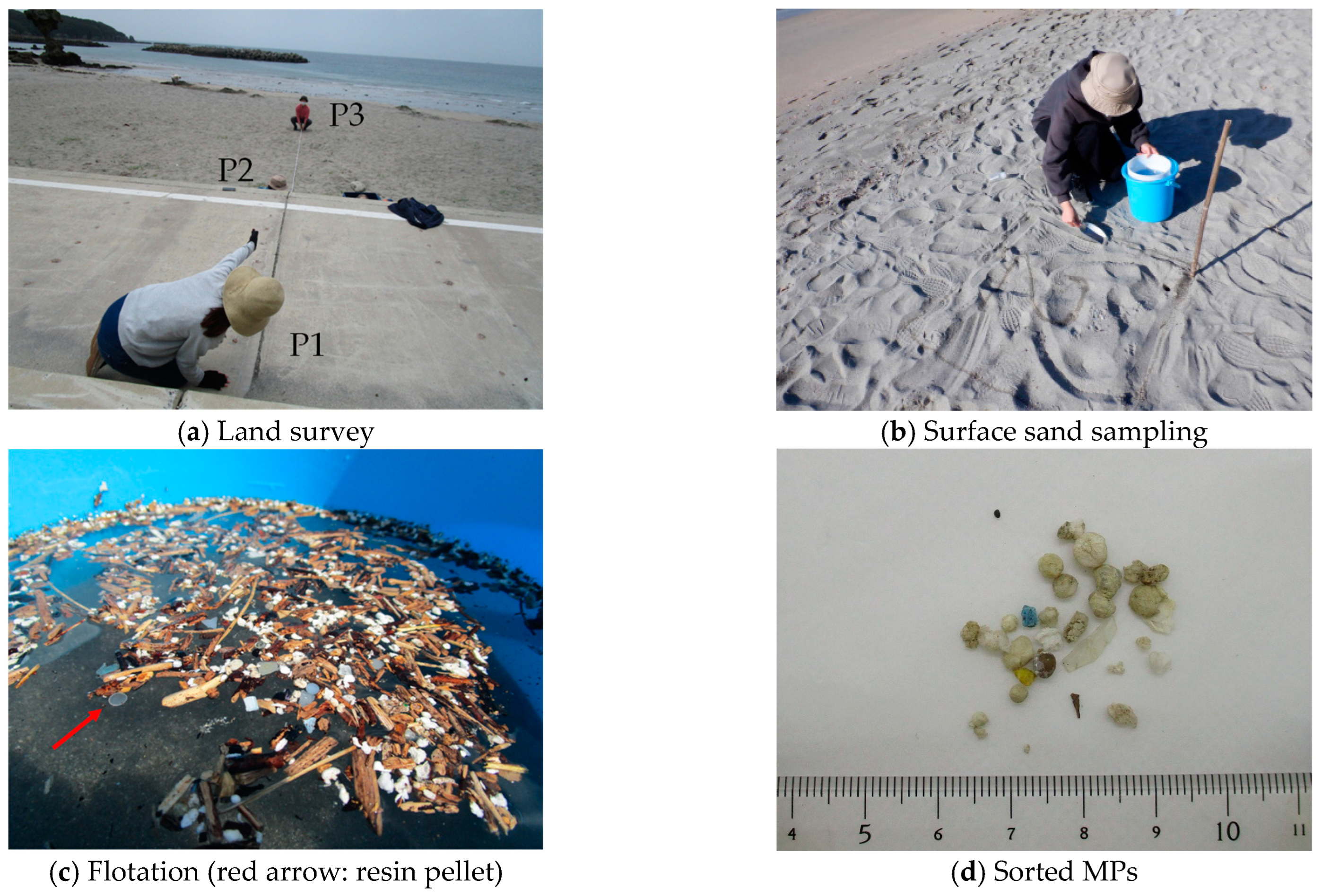
A flow chart of the investigation procedure is shown in Figure 2. A land survey is required to identify or record the sampling point location (Figure 3a). The purpose of surveying is twofold. First, for multiple periodic investigations, we survey and determine the sampling square at a fixed location (fixed spot). This will eliminate the concern of MPs fluctuation due to differences in location and make it easier to clarify seasonal variations and accumulation rates. Next, if the location of the sampling square changes depending on the investigation date, the location should be recorded. For example, we can visually determine the location where MPs are relatively abundant, such as on the high tide line or in a blowhole (hot spot), and record the location by surveying that sampling point. In other words, for a fixed spot investigation, we survey first and then drive in a stake (hereinafter referred to as “staking after survey”), and for a hot spot investigation, we survey after driving in a stake (hereinafter referred to as “survey after staking”).
Because our goal is to determine the MPs content in sand, the sand itself is not needed. However, as there was no available means of recovering MPs alone, we first collected the surface sand. MPs are plastic fragments measuring 5 mm or less, so a sieve with a 5 mm aperture was used to remove large particles (Figure 3b). The MPs content per area is determined by measuring the area of the sampling square or by making a 1 m2 square in advance. If the weight of the collected sand is measured, the MPs content per sand weight can be reported if the MPs weight is negligible.
The time available to work in the field is limited. In addition, there may be difficulties owing to weight or conservation concerns in bringing sand back from the beach. Considering these factors, we try to extract MPs from sand quickly in the field. Therefore, in this study, we conducted sorting by flotation using seawater or tap water. For example, sand was placed in a bucket filled with approximately 5 L of seawater, and the sand and the seawater were stirred together a little at a time and allowed to stand for approximately 3 min. Floating matter (Figure 3c) was scooped out with a ladle along with seawater and brought back to the laboratory in a plastic bottle or plastic bag.
The floating matter brought back to the laboratory contained particles other than MPs. MPs were sorted from the floating matter using the method described in Section 2.5, washed with tap water, dried, and weighed (Figure 3d).
2.2. Land Survey
NOAA has introduced a surveying method that uses GPS on smartphones, a tape measure, and measuring wheels [30]. As of 2023, the margin of error is a few meters [34], and GPS can be used only if this error can be tolerated in a MPs investigation. Advanced GPS equipment is expensive, so we do not deal with it in this study. Because this study targets high school students, inexpensive and easily available surveying instruments will be used.
A 50 and 10 m tape measure was used to measure distances, and cardboard was used to measure right angles (Figure 4a). The position of the stake (xi, yi) with respect to the reference point, the origin (0, 0), was obtained (Figure 4b). Because a novice surveyor used simple tools such as a tape measure and cardboard, there would be errors in the location of the stakes (xi, yi) in both staking after survey and survey after staking. However, no matter how expensive the surveying instruments are, errors will still occur. In the staking after survey, the position of the driven stake will be off from the true position, and in the survey after staking, there will be errors in the data of the recorded stake positions (xi, yi). The purpose of the survey experiment is to evaluate these errors. Six sets of surveys were repeated twice with three persons rotating roles at Beach A. For staking after the survey, six stakes were driven by surveying 20.00 m in the y-axis direction and 5.00 m in the x-axis direction (the smallest unit was 0.01 m). The six stakes were located in a small plot, and 30 cm rulers were placed at right angles around them. Photographs were taken directly above, and the coordinates of the six stakes were recorded by considering the intersection of the rulers as a temporary origin (Figure 4c). For the survey after staking, a stake was driven approximately 20 m in the y-axis direction and 5 m in the x-axis direction, and six measurements were made (the smallest unit was 0.01 m). Figure 4d shows the six coordinates and the average coordinate. Staking after the survey yields coordinates (xi, yi) (i = 1, 2, 3, 4, 5, 6) for the six stakes, and six points exist when we put dots in the xy coordinates. The survey after staking yields six coordinates (xi, yi). In this case, there is one stake and its position is fixed, but there are six surveyed coordinates. Therefore, if we enter the surveyed coordinates in the xy coordinates, there are six points as in the case of staking after the survey. From these six coordinates, the average coordinate (xave, yave) is obtained.
The distance ei, i.e., the deviation, from the average coordinate to each of the six coordinates is calculated from the Pythagorean theorem.
If this distance is squared, the deviation is squared. These six ei2 are summed to obtain the sum of squares. Dividing this by the degrees of freedom (n = 6, n − 1 = 5) gives the unbiased variance s2.
Because the square root of the unbiased variance is not an estimator of the population standard deviation σ, σ is estimated by dividing s by the correction factor c4 (0.952 for n = 6) obtained from the gamma function.
Dividing the population standard deviation σ by the distance from the origin to the average coordinate lave gives the coefficient of variation CV.
(xave, yave) = 1/n Σ (xi, yi)
ei = {(xi − xave)2 + (yi − yave)2}0.5
s2 = 1/(n − 1) Σ ei2
σ = s/c4
CV = σ/lave
In the staking after survey, we assumed a distance of 20.00 m in the y-axis direction and 5.00 m in the x-axis direction, i.e., (202 + 52)0.5 = 20.6 m, and in the survey after staking, the distance from the origin to the average coordinate was considered as lave. This coefficient of variation expresses the variability of the survey results. In the staking after the survey, the measurement error by the 30 cm ruler was also introduced; however, it was ignored because it was much smaller than lave = 20.6 m.
2.3. Heavy Liquid Sorting
Because the density of polyethylene (PE) and polypropylene (PP), the first and second most produced plastics, is less than 1 g/cm3 if sand containing them is added into tap water (density: approximately 1 g/cm3) or seawater (density: approximately 1.02 to 1.03 g/cm3) [32], sand (density: 2 g/cm3 or higher) will sink and PP and PE will float. Thus, PP and PE can be easily sorted from sand. However, polyvinyl chloride (PVC) and polyethylene terephthalate (PET) cannot be sorted from sand because their density exceeds 1 g/cm3 and thus they sink in tap water or seawater. In other words, the flotation sorting using tap water or seawater is not applicable to plastics with densities exceeding 1 g/cm3. Considering the phenomenon of plastics drifting across oceans, it is justifiable to target only plastics with a density of less than 1 g/cm3 for investigation. However, plastics that are hollow (e.g., recapped plastic bottles), composite materials (e.g., fishing nets with floats), and plastics originating from the landward side, all of which have densities exceeding 1 g/cm3, can also be present on beaches. If heavy liquids with densities exceeding 1 g/cm3 are used, PVC and PET will also float and thus can be sorted. However, in the author’s experience from several investigations, most of the MPs in the sand appeared to be collected by flotation sorting using tap water or seawater. As tap water and seawater are readily available on-site and almost free of charge, we would like to complete the flotation sorting with these liquids. After flotation sorting of MPs in sand with tap water or seawater, is there any plastic with a density greater than 1 g/cm3 remaining in the sand? If the amount of MPs recovered by the heavy liquid is negligible compared with the amount of MPs recovered by the tap water or seawater, the flotation sorting method using only tap water or seawater is justified.
At Beach A, MPs in the sand surface layer (0.5 cm depth) were sorted with seawater, and then calcium chloride (TOKUYAMA, snow-melting agent) was added to the seawater containing sand until saturation (Figure 5a) to create a heavy liquid with a density of approximately 1.3 to 1.4 g/cm3 (approximately 1 kg- snow-melting agent/L-water), at which time the MPs that finally floated were collected. The density of the calcium chloride solution exceeds that of the sodium chloride solution (1.2 g/cm3) [27]. Twelve experiments at hot spots were conducted at the sites. The density of the liquid was measured with a buoy (AS ONE, polycarbonate density meter).
2.4. Distribution in Depth
When conducting field investigations on sandy beaches, MPs were noticeably found on the surface of sand. There is a tradeoff between area and depth. In this study, the sampling depth was shallower by setting a larger sampling area. MPs were usually collected by sampling to a depth of approximately 0.5 cm from the surface layer of sand at a sampling square of 1 m2. This sand could fit into one 10-L bucket. In many cases, no MPs were found in the surface layer of the sand after sampling. If we assume that the original plastic of the MPs on the beach has drifted across the ocean, we can imagine how the plastic is carried by the waves and left on the sand at high tide. In other words, it is natural that plastics and MPs exist in abundance on the sand. When investigating the MPs content of sand, it is quite hard work to dig deep [32], so we want to collect only the surface layer of sand. This sampling method may also be justified by the fact that MPs are found mostly in the surface layer. Is it appropriate to collect only the surface layer of sand for the MPs study? In other words, when taking into consideration the MPs distribution of multiple layers in the depth direction, do the MPs in the surface layer account for most of the total MPs?
Multiple layers of sand were collected (at depths of 0–0.5 cm and 0.5–5 cm, and every 5 cm thereafter), and the MPs contained in the sand were measured. One side of the sampling square is 38 cm so that one 10-L bucket can hold 5 cm-thick sand. Experiments were conducted at three sites at hot spots in Beach A. Strings were placed on the ground surface to mark the 0 cm depth. A shovel was used to dig out the sand around a square prism with 38 cm sides, and a plastic plate was used to cut out the prism (Figure 5b). A 5 cm-deep layer was scooped out with the same plastic plate. In addition, at Beaches C and D, MPs were measured by collecting approximately 0.5 cm-deep sand from the surface layer of the 1 m2 sampling square and then collecting approximately 0.5 cm-deep sand from the layer immediately below the surface layer.
2.5. Sedimentation of Wood Particles by Boiling
Floating matter contained not only MPs but also plants, animals, and pumice. Wood particles were particularly abundant. Although MPs can be visually sorted out, the need for subjective judgment is a concern. Wood particles floated on the seawater in the bucket, but not on the seawater at the study site. The true density of the wood is 1.40–1.47 g/cm3 [35]. The author has hypothesized that the wood floated owing to the low bulk density of the dry wood (0.22–0.81 g/cm3). If the wood is boiled to promote wetting, the wood will sink and only the MPs will float. The fact that the wood sinks by boiling was conceived from the author’s unsuccessful experiments on MPs. In this way, the MPs content is considered the amount of floating matter after boiling.
The floating matter was stored in plastic bottles or plastic bags and transported back to the laboratory. The floating matter was transferred to beaker A with the seawater (Figure 5c) and boiled on a hot plate at a set temperature of 140 °C for 3 h with a watch glass on top. After boiling, the (primary) floating matter was separated into secondary floating matter and sediment (Figure 5d). Prepare Beaker B with tap water was prepared. After boiling, the floating matter in beaker A after boiling was scooped out with a spoon and placed in beaker B. The floating matter was stirred and washed. The liquid remaining in beaker A was decanted and discarded, and tap water was repeatedly added and stirred to wash the sediments. The washed floating matter and sediments were transferred to stainless steel trays and dried in a dryer at 80 °C for at least one night. The weights of the dried matter were measured on an electronic balance. The MPs were visually removed and separated into floating MPs, other floating matter, sedimented MPs, and other sediment (Figure 6). The weight of each was measured on an electronic balance. This was conducted at Beaches A, B, C, and D at fixed and hot spots.
2.6. Lower Limit of Quantification
GESAMP recommends that quality assurance of MPs analysis be performed by reporting the results of spiked recovery tests [32]. Dou et al. (2021) reported a recovery rate of more than 57% as a result of recovery tests of MPs in soil [36]. This would allow us to express the accuracy and precision of the measurement.
However, to prove the correctness of the measurement, a lower limit of quantification must be given in addition to the recovery rate. When the author repeated the measurement of MPs in the sand, many results of 0 mg were obtained. In this study, MPs in the sand were collected by flotation sorting, boiled and dried, visually sorted for MPs, and weighed on weighing paper. Even if MPs could not be confirmed, the weighing was completed by the act of placing the non-existent MPs on the weighing paper. At this point, the weight of MPs was 0 mg. However, owing to the procedure for sample collection and measurement, there is a lower limit of quantification (LLOQ), and the LLOQ should be noted and reported instead of 0 mg as the measured value. A dummy value referring to the LLOQ should be used instead of 0 mg when taking the average of multiple measured values at low concentrations. Therefore, the LLOQ for the method used in this study, in which 1 m2 of sand was collected in a bucket and MPs were collected and measured by flotation sorting with seawater, was determined.
The method introduced by Mermet (2008) for determining the LLOQ on the basis of an evaluation of the repeatability of actual measurements [37] was used as a reference. Standard samples (MPs) of several set weights were prepared within the range including the estimated LLOQ. The standard samples were made from a PP beverage bottle cap (density 0.93 g/cm3) ground with a grinder to a powder of less than 1 mm. Six different standard samples of the same set weight (approximately 8, 15, 22, 30, 37, and 44 mg) were prepared, three each. A bucket of 1 m2 of clean (presumably very low MPs) sand (0.5 cm deep) from Beach A was collected and loaded with the standard samples. MPs were collected, boiled, and measured by flotation sorting with seawater.
Because there are three standard samples at the same set weight (added amount), three recoveries are obtained. We assume a model in which a smaller addition makes recovery and measurement more difficult and a larger addition makes it easier. Then, if the addition is small, the measured value (recovery) will vary greatly from the average value, and if the addition is large, the measured value will vary little from the average value. The average and the unbiased variance of these three recovery values are obtained, and the square root of the unbiased variance is divided by the average to obtain the coefficient of variation. In other words, if the added amount is small, the coefficient of variation is large, and if the added amount is large, the coefficient of variation is small. The relationship between the addition x and the coefficient of variation y is regressed by some mathematical formula. In this case, a power function (Equation (6)) is used.
The actual added amount x and the coefficient of variation y are plotted on a scatter plot, the regression curve (Equation (6)) is fitted, and the coefficients a and b are obtained using Excel’s graphing function (least squares method). The equation is transformed to find the weight x (Equation (7)).
An acceptable coefficient of variation y is set and substituted, and coefficients a and b are also substituted to obtain the weight of minimum MPs added x (LLOQ) that satisfies the required coefficient of variation.
y = ax−b
x = (y/a)(−1/b)
3. Results
3.1. Errors in Simple Survey
An example of the results of staking after the survey (first survey) is shown in Table 1. The coefficient of variation CV is 0.43% for the first survey and 0.60% for the second survey. The results of the survey after staking are 0.93% for the first survey and 0.90% for the second one. Using the maximum value of approximately 1%, this means that when driving a large number of stakes at a distance of approximately 20 m or surveying an existing stake a large number of times, assuming a normal distribution, 70% of the deviations are within approximately 20 cm (20 × 1/100 = 0.2 m).
3.2. Heavy Liquid Sorting
The results of heavy liquid sorting (n = 12) are shown in Figure 7 (Supplementary Materials). Floating MPs in seawater (light MPs) average 392 mg-MPs/m2-sand and those in heavy liquid (heavy MPs) average 48 mg-MPs/m2-sand. Both light and heavy MPs are recovered from sand collected from a single sampling square. Therefore, the Wilcoxon signed-rank test is performed, and light MPs are found to be significantly more common than heavy MPs (p < 0.05). On average, light MPs account for 89% and heavy MPs, for 11% of all MPs (light + heavy MPs).
3.3. Distribution in Depth Direction
The distribution of MPs in the depth direction is shown in Figure 8a (Supplementary Materials). In the first investigation, sampling is performed to a depth of 40 cm, and in the second and third investigations, sampling to a depth of 50 cm is performed. In the first investigation, 99% of the total MPs are in the first layer (0 to 0.5 cm) and in the second and third investigations, 50% and 49% of the total MPs are in the first layer. The total amounts of MPs collected in the three investigations differ (19000, 6800 and 1300 mg for first, second and third). The total weights of MPs in the second and third investigations are 35% and 6% of that in the first investigation, respectively. If the overall weight of MPs is small, the presence of even a few MPs in deeper areas will reduce the percentage in the first layer. Therefore, by simply averaging the MPs content per layer of the three investigations, we find that the first layer contains 85% of the total MPs.
At Beaches C (n = 12) and D (n = 12), for MPs present to a depth of 1 cm, at least 70% are present in the surface layer down to 0.5 cm depth (Figure 8b, Supplementary Materials). When the total MPs content for the 12 sites is calculated, more than 95% of the MPs are present in the surface layer down to 0.5 cm depth at both beaches.
3.4. Sedimentation of Wood Particles by Boiling
For all samples (n = 189), floating matter, sedimented matter, and total matter after boiling weigh 647 g, 460 g, and 1107 g, respectively (Figure 9a, Supplementary Materials). After visual sorting, floating MPs, other floating matter, sedimented MPs, and other sediments, and total weigh 309, 312, 2, 455, and 1078 g, respectively. The total weights are almost equal. The MPs that sink after boiling account for 0.8% of the total MPs, which is a negligible amount. The amount of floating matter is 2.1 times that of the total MPs.
The relationship between total MPs and floating matter is shown in Figure 9b (Supplementary Materials). The red line is the theoretical line showing MPs:floating = 1:1. Almost all points are above the theoretical line. The regression line for all samples is y = 1.88x + 0.33 (r2 = 0.67). Here, a submarine volcanic eruption on the Ogasawara Islands occurred in August 2021, and a large amount of pumice drifted into the area around Okinawa southwest of Kyushu in October. Subsequently, the pumice stone drift was observed at other sites as well. In this study, large quantities of pumice were found on Beach B in September 2022 and on Beach D in December 2022. The pumice did not settle at all by boiling. Samples containing this pumice (n = 65) are indicated by orange circles in the figure. It can be seen that it deviates significantly upward from the theoretical line.
For the sample without pumice (n = 124), floating matter, sedimented matter, and total matter after boiling weigh 184 g, 217 g, and 400 g, respectively. After visual sorting, the floating MPs, other floating matter, sedimented MPs, other sediments, and total weigh 125, 54, 1, 216, and 397 g, respectively. The total weights are almost equal. The MPs that sink after boiling account for 1.1% of the total MPs, which is negligible. The amount of floating matter is 1.5 times that of the total MPs. The regression line is y = 1.21x + 0.25 (r2 = 0.97).
3.5. Lower Limit of Quantification
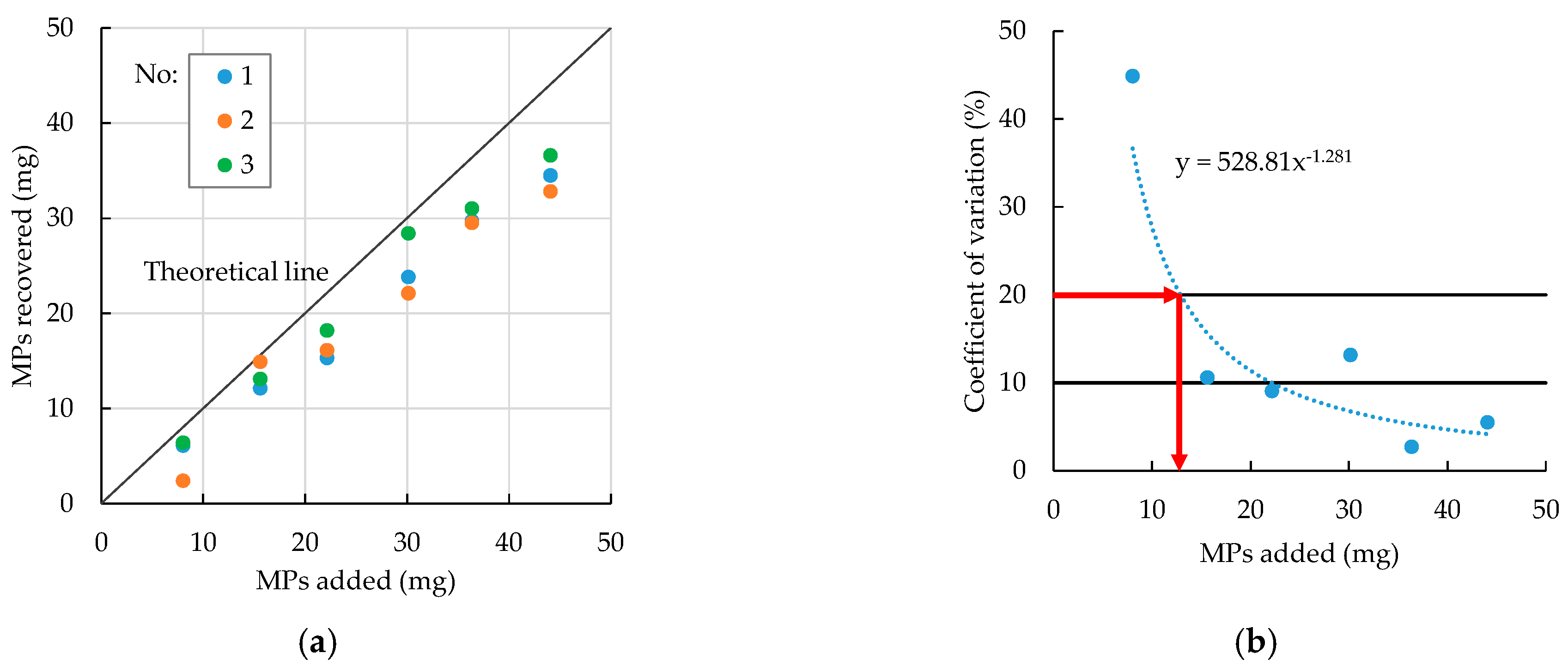
The relationship between the amount of MPs added and the amount recovered is shown in Figure 10a (Supplementary Materials). The diagonal line is the theoretical line indicating that the amount of MPs added is equal to the amount recovered (100% recovery). All the recoveries are below the theoretical line, indicating that the recovery is less than 100% (62% at 8 mg added, a minimum of 75% otherwise). The observed values on the scatter plot appear to be aligned in a straight line with a right ascension.
4. Discussion
4.1. Survey Accuracy When Using Simple Survey Tools
When novice persons surveyed a distance of approximately 20 m several times using simple tools, such as a tape measure and cardboard, using immovable natural and artificial objects in the study site as landmarks, 70% of the deviations were within approximately 20 cm. The accuracy of the survey is sufficient to drive stakes at the same sampling points as the previous investigations and to mark the survey points on the map.
4.2. MPs That Sink in Seawater
Of the MPs contained in the sand, 11% could be recovered not with seawater (density 1.03 g/cm3) but only with heavy liquid (minimum density 1.33 g/cm3). In other words, 89% of MPs could be recovered using only seawater. Therefore, if workload reduction is desired, recovery of MPs by seawater only is acceptable.
The six major types of plastics are PE, PP [38], PVC, polyurethane (PUR), polystyrene (PS), and PET [39]. PE (36%), PP (21%), and PVC (12%), followed by PET, PUR, and PS (<10% each), are the major categories in global non-fiber plastics production [3]. These groups are responsible for 92% of the production of plastics. Approximately 42% of non-fiber plastics are used for packaging, mainly PE, PP, and PET [3].
The densities of PP, PE, and PVC are 0.90–0.92, 0.91–0.95, and 1.16–1.30 g/cm3, respectively [32], so PP and PE float in seawater. Although there is no guarantee that the breakdown of plastics produced will match the breakdown of MPs on beaches, it is expected that PP and PE will account for the majority of MPs on beaches. Of the MPs found on beaches, PP and PE account for 89% [40], 87% [41], 77% [42], 74% (PS: 25%) [43], 59% (PS: 33%) [44], and 57% (PS: 38%) [45]. PS may be Styrofoam [44]. Styrofoam has a density of 0.02–0.64 g/cm3 [32] and thus floats in seawater. This means that the majority of MPs found on sandy beaches are floating in seawater.
4.3. MPs Distribution in Depth
On the basis of the results of the three investigations at Beach A, it became clear that an investigation of MPs content by sampling 0.5 cm of the surface layer of sand could explain more than half of the MPs content when the sand was sampled to a depth of approximately 50 cm below the surface layer. Therefore, if workload reduction is desired, sand sampling only in the surface layer is acceptable.
Duncan et al. (2018) studied the distribution of MPs in sand to a depth of 60 cm in Cyprus and found that 42% of all MPs were found in the surface layer [46]. Sewwandi et al. (2022) studied the distribution of MPs in sand at seven locations to a depth of 1 m in Sri Lanka and found MPs in the surface layer at five locations [40]. Nhon et al. (2022) studied the distribution of MPs in sand to a depth of 7 cm in Vietnam and found that 82% of all MPs were found in the surface layer (2 cm) [45]. This confirms that MPs in the surface layer account for the majority of the MPs.
On the other hand, there are reports that MPs were found at greater depths as well. Rather than being present in high concentrations at any depth, they are present in high concentrations at certain depths [40,47]. In this study, too, MPs were found in uniquely high concentrations at depths of 20 cm and 35 cm at No. 2 in Figure 8a. No. 2 is located high on the backshore, where runoff sand to the sea was returned and deposited by heavy equipment. Thus, the No. 2 surface layer was approximately 1 m higher at the time of investigation than before it. No. 1 and No. 3 are located on the foreshore. This phenomenon of high concentration of MPs may be due to some events, such as sand movement.
4.4. Error in Considering Floating Matter as MPs after Boiling
Unlike the visual sorting of MPs, the boiling process does not require experience and skill and is, therefore, easy to standardize. Therefore, the author would like to propose a method in which floating matter after boiling is considered as MPs. Because of the presence of wood particles and pumice that do not sink even after boiling, the boiling method estimates approximately twice the amount of MPs compared with the true amount of MPs. However, pumice stone drift is an isolated case. If there is no concern about pumice contamination, the overestimation is approximately 1.5 times. Boiling takes 3 h, but several samples can be processed simultaneously. If this error can be tolerated, the boiling method is a simple method for estimating MPs. The author originally assumed the presence of floating inorganic matter such as pumice, and planned to measure the loss on ignition of floating matter as the final method to determine the weight of MPs. However, because the author decided to keep the samples in consideration of the possibility of measuring the number of particles and determining their materials of origin, the author did not perform heat treatment.
4.5. Lower Limit of Quantification of MPs Using the Measurement Method Presented in This Study
The coefficients of variation obtained from several recoveries for a given MP added are shown in Figure 10b (Supplementary Materials). The coefficients in Equation (6) are a = 528.8 and b = 1.281. From Equation (7), if coefficients of variation y = 10% or 20% are allowed, the minimum MPs added x are 22 or 13 mg, respectively. In this experiment, MPs are added to and collected from the sand in the surface layer of 1 m2 of sandy beach, so 22 and 13 mg-MPs/m2-sand are the LLOQs per area as it is. In addition, the average dry weight of sand collected from 1 m2 in this experiment is 5.4 kg-sand/m2-sand, so dividing by this, 4 and 2 mg-MPs/kg-sand are the LLOQs per weight. In this study, as the development of the MPs investigation method is in its initial stage, a lenient standard (coefficient of variation of 20%) is adopted, and 13 mg-MPs/m2-sand and 2 mg-MPs/kg-sand are considered to be the LLOQs. In addition, measured values below the LLOQs are replaced with the LLOQs.
MPs measured in 5 L of tap water and seawater only were <1 mg (n = 6).
4.6. Problems of This Study, Future Research
Land surveys required a lot of labor and time. The author looks forward to the improved accuracy of smartphone GPS that will require only one person for land survey.
It is obvious that it is better to use heavy liquid rather than seawater to investigate all MPs. The author has not been able to measure heavy MPs with a density higher than that of the heavy liquid used in this study. At least the same volume of heavy liquid as sand is required, and the preparation of heavy liquid is costly. We would like to see the accumulation of data showing that the amount of heavy plastics requiring heavy liquid is negligible.
It is not guaranteed that MPs will not be present in deep areas. If possible, sand should be excavated to depths of 50 cm occasionally. Beach cleaning is often conducted at Beach A, and the runoff sand is returned with heavy equipment. It is ironic that beach management activities make MPs investigations difficult. The MPs should be collected before moving the sand to avoid burying the MPs. It is possible that there is heavy plastic that does not float in seawater at great depths, but this was not measured in this study. The heavy plastic should be measured.
MPs in the sample after boiling were visually sorted, but there was no guarantee that they were purely MPs. The author would like to acquire a list of items that can be easily misidentified as MPs. The weight loss of MPs due to boiling should be evaluated.
The LLOQ test expresses a part of precision but does not express accuracy. As shown in Figure 10a, the low recovery rate means that the accuracy is low. In the future, we should conduct addition-recovery tests over a wide range of MPs weights. In addition, the plastics used were selected from a single type of material and adjusted to a narrow particle size range of 1 mm or less. Data should be accumulated for other samples.
In this study, the material type of MPs has not been determined, so spectral analysis needs to be carried out. This study was carried out only in a limited number of regions in Japan. It should be conducted in other regions and in other countries to assess the variability of results.
4.7. Significance of This Study
The accuracy of simple MPs investigation methods could be determined. If data on the amount of MPs in the environment could be collected by high school students as well as professional researchers, long-term trends in MPs degradation could be clarified.
Another possible method is to remove sand with a sieve and measure MPs remaining on the sieve. However, the method used in this study has the advantage of not excluding small MPs. Calcium chloride is one of the major constituents of seawater, so there is little risk of environmental contamination during sorting operations on a beach. Calcium chloride for laboratory use is expensive (3000 yen per 0.5 kg, FUJIFILM Wako Chemicals), whereas calcium chloride for melting ice on roads is inexpensive (4000 yen per 25 kg). The cost of salt is 2500 yen per 25 kg. Although plastic instruments were used, no contamination was observed because there were no outliers in the experimental data for the LLOQ test. If the measurement is made near the LLOQ set in this study, there should be no concern about contamination. However, the author does not recommend the use of plastic products because of the possibility of large contamination.
5. Conclusions
The accuracy of the simple MPs investigation method can be explained as follows.
- (1)
- Sufficient accuracy is achieved by the land survey that uses a tape measure and a piece of cardboard as simple tools, and immovable natural and artificial objects in the study site as landmarks. When multiple surveys of approximately 20 m distance are performed, the maximum coefficient of variation is approximately 1%, i.e., 70% of the deviations are within approximately 20 cm.
- (2)
- If workload reduction is desired, recovery of MPs by seawater only is acceptable. Eighty-nine percent of MPs can be recovered with seawater only.
- (3)
- If workload reduction is desired, sand sampling only in the surface layer is acceptable. An investigation of MPs content by sampling 0.5 cm of the surface layer of sand can explain more than half of the MPs content when the sand is sampled to a depth of approximately 50 cm below the surface layer.
- (4)
- If workload reduction is desired, a method in which the recovered MPs are not visually sorted, but the floating matter after boiling is considered as MPs is acceptable. If there is no concern about pumice contamination, the overestimation is approximately 1.5 times.
- (5)
- Simple laboratory equipment such as buckets, sieves, seawater, hot plates, dryers, and electronic balances can achieve lower limits of quantification of MPs of 13 mg-MPs/m2-sand and 2 mg-MPs/kg-sand.
Existing and simple MPs investigation methods that can be conducted by high school students have the accuracy shown above. This study will stimulate MPs surveys by citizens, including high school students, and increase the data accumulation rate.
In this study, instruments made of plastic material were also used as accessible tools for high school students. This is because the author was interested in the lower limit of quantification when plastic instruments were used. However, in order to obtain accurate results for the analysis of MPs, instruments made of plastic material, which are the raw material for MPs, must be eliminated and their use is not recommended. Instruments made of glass or metal should be used.
Supplementary Materials
The following supporting information can be downloaded at: https://www.mdpi.com/article/10.3390/microplastics2030024/s1.
Funding
This research was supported by a Grant-in-Aid for Scientific Research C (20K12208) from the Japan Society for the Promotion of Science (JSPS). The APC was funded by the Institute of Integrated Sciences and Technology, Nagasaki University.
Institutional Review Board Statement
Not applicable.
Data Availability Statement
Data are available in the Supplementary Materials.
Acknowledgments
The authors would like to thank Soichiro YAMAMOTO, Hayata GOTO, Toshiki SATO, Yui CHINJU, and Yukari TOKIYASU.
Conflicts of Interest
The author declares no conflict of interest. The funder had no role in the design of the study; the collection, analyses or interpretation of data; the writing of the manuscript or the decision to publish the results.
References
- Willis, K.A.; Eriksen, R.; Wilcox, C.; Hardesty, B.D. Microplastic Distribution at Different Sediment Depths in an Urban Estuary. Front. Mar. Sci. 2017, 4, 419. [Google Scholar] [CrossRef]
- Jambeck, J.R.; Geyer, R.; Wilcox, C.; Siegler, T.R.; Perryman, M.; Andrady, A.; Narayan, R.; Law, K.L. Plastic waste inputs from land into the ocean. Science 2015, 347, 768–771. [Google Scholar] [CrossRef] [PubMed]
- Geyer, R.; Jambeck, J.R.; Law, K.L. Production, use, and fate of all plastics ever made. Sci. Adv. 2017, 3, e1700782. [Google Scholar] [CrossRef] [PubMed]
- Barnes, D.K.A.; Galgani, F.; Thompson, R.; Barlaz, M. Accumulation and fragmentation of plastic debris in global environments. Philos. Trans. R. Soc. B Biol. Sci. 2009, 364, 1985–1998. [Google Scholar] [CrossRef] [PubMed]
- Browne, M.A.; Galloway, T.; Thompson, R. Microplastic–an emerging contaminant of potential concern? Integr. Environ. Assess. Manag. 2007, 3, 559–561. [Google Scholar] [CrossRef] [PubMed]
- Andrady, A.L. Microplastics in the marine environment. Mar. Pollut. Bull. 2011, 62, 1596–1605. [Google Scholar] [CrossRef] [PubMed]
- Cole, M.; Lindeque, P.; Halsband, C.; Galloway, T.S. Microplastics as contaminants in the marine environment: A review. Mar. Pollut. Bull. 2011, 62, 2588–2597. [Google Scholar] [CrossRef]
- Mato, Y.; Isobe, T.; Takada, H.; Kanehiro, H.; Ohtake, C.; Kaminuma, T. Plastic resin pellets as a transport medium for toxic chemicals in the marine environment. Environ. Sci. Technol. 2001, 35, 318–324. [Google Scholar] [CrossRef]
- Frias, J.P.; Sobral, P.; Ferreira, A.M. Organic pollutants in microplastics from two beaches of the Portuguese coast. Mar. Pollut. Bull. 2010, 60, 1988–1992. [Google Scholar] [CrossRef]
- Bellas, J.; Martinez-Armental, J.; Martinez-Camara, A.; Besada, V.; Martinez-Gomez, C. Ingestion of microplastics by demersal fish from the Spanish Atlantic and Mediterranean coasts. Mar. Pollut. Bull. 2016, 109, 55–60. [Google Scholar] [CrossRef]
- Rochman, C.M.; Hoh, E.; Hentschel, B.T.; Kaye, S. Long-term field measurement of sorption of organic contaminants to five types of plastic pellets: Implications for plastic marine debris. Environ. Sci. Technol. 2012, 47, 1646–1654. [Google Scholar] [CrossRef]
- Rochman, C.M.; Hoh, E.; Kurobe, T.; Teh, S.J. Ingested plastic transfers hazardous chemicals to fish and induces hepatic stress. Sci. Rep. 2013, 3, 3263. [Google Scholar] [CrossRef] [PubMed]
- Vandermeersch, G.; Van Cauwenberghe, L.; Janssen, C.R.; Marques, A.; Granby, K.; Fait, G.; Kotterman, M.J.; Diogene, J.; Bekaert, K.; Robbens, J.; et al. A critical view on microplastic quantification in aquatic organisms. Environ. Res. 2015, 143, 46–55. [Google Scholar] [CrossRef] [PubMed]
- Lusher, A.L.; McHugh, M.; Thompson, R.C. Occurrence of microplastics in the gastrointestinal tract of pelagic and demersal fish from the English Channel. Mar. Pollut. Bull. 2013, 67, 94–99. [Google Scholar] [CrossRef] [PubMed]
- Tanaka, K.; Takada, H.; Yamashita, R.; Mizukawa, K.; Fukuwaka, M.; Watanuki, Y. Accumulation of plastic-derived chemicals in tissues of seabirds ingesting marine plastics. Mar. Pollut. Bull. 2013, 69, 219–222. [Google Scholar] [CrossRef]
- Ng, K.L.; Obbard, J.P. Prevalence of microplastics in Singapore’s coastal marine environment. Mar. Pollut. Bull. 2006, 52, 761–767. [Google Scholar] [CrossRef]
- Corcoran, P.L.; Biesinger, M.C.; Grifi, M. Plastics and beaches: A degrading relationship. Mar. Pollut. Bull. 2009, 58, 80–84. [Google Scholar] [CrossRef]
- Turner, A.; Holmes, L. Occurrence, distribution and characteristics of beached plastic production pellets on the island of Malta (central Mediterranean). Mar. Pollut. Bull. 2011, 62, 377–381. [Google Scholar] [CrossRef] [PubMed]
- Martins, J.; Sobral, P. Plastic marine debris on the Portuguese coastline: A matter of size? Mar. Pollut. Bull. 2011, 62, 2649–2653. [Google Scholar] [CrossRef]
- Hidalgo-Ruz, V.; Thiel, M. Distribution and abundance of small plastic debris on beaches in the SE Pacific (Chile): A study supported by a citizen science project. Mar. Environ. Res. 2013, 87–88, 12–18. [Google Scholar] [CrossRef]
- Mathalon, A.; Hill, P. Microplastic fibers in the intertidal ecosystem surrounding Halifax Harbor, Nova Scotia. Mar. Pollut. Bull. 2014, 81, 69–79. [Google Scholar] [CrossRef] [PubMed]
- Masura, J.; Baker, J.; Foster, G.; Arthur, C. Laboratory Methods for the Analysis of Microplastics in the Marine Environment: Recommendations for Quantifying the Synthetic Particles in Water and Sediments; NOAA Marine Debris Division: Silver Spring, MA, USA, 2015. [Google Scholar]
- Wessel, C.C.; Lockridge, G.R.; Battiste, D.; Cebrian, J. Abundance and characteristics of microplastics in beach sediments: Insights into microplastic accumulation in northern Gulf of Mexico estuaries. Mar. Pollut. Bull. 2016, 109, 178–183. [Google Scholar] [CrossRef] [PubMed]
- Crichton, E.M.; Noël, M.; Gies, E.A.; Ross, P.S. A novel, density-independent and FTIR-compatible approach for the rapid extraction of microplastics from aquatic sediments. Anal. Methods 2017, 9, 1419–1428. [Google Scholar] [CrossRef]
- Maes, T.; Jessop, R.; Wellner, N.; Haupt, K.; Mayes, A.G. A rapid-screening approach to detect and quantify microplastics based on fluorescent tagging with Nile red. Sci. Rep. 2017, 7, 44501. [Google Scholar] [CrossRef]
- Quinn, B.; Murphy, F.; Ewins, C. Validation of density separation for the rapid recovery of microplastics from sediment. Anal. Methods 2017, 9, 1491–1498. [Google Scholar] [CrossRef]
- Hidalgo-Ruz, V.; Gutow, L.; Thompson, R.C.; Thiel, M. Microplastics in the Marine Environment: A Review of the Methods Used for Identification and Quantification. Environ. Sci. Technol. 2012, 46, 3060–3075. [Google Scholar] [CrossRef]
- Cheshire, A.C.; Adler, E.; Barbière, J.; Cohen, Y.; Evans, S.; Jarayabhand, S.; Jeftic, L.; Jung, R.T.; Kinsey, S.; Kusui, E.T.; et al. UNEP/IOC Guidelines on Survey and Monitoring of Marine Litter; UNEP Regional Seas Reports and Studies. 186 (IOC Technical Series No. 83); United Nations Environment Programme: Nairobi, Kenya, 2009; p. 120. [Google Scholar]
- Wenneker, B.; Oosterbaan, L.; Intersessional Correspondence Group on Marine Litter (ICGML). Guideline for Monitoring Marine Litter on the Beaches in the OSPAR Maritime Area; OSPAR Commission: London, UK, 2010; p. 15. [Google Scholar] [CrossRef]
- Burgess, H.K.; Herring, C.E.; Lippiatt, S.; Lowe, S.; Uhrin, A.V. NOAA Marine Debris Monitoring and Assessment Project Shoreline Survey Guide; NOAA Technical Memorandum. NOSOR&R 56: Silver Spring, MA, USA, 2021; p. 20. Available online: https://repository.library.noaa.gov/view/noaa/33282 (accessed on 18 June 2023).
- Galgani, F.; Hanke, G.; Werner, S.; Oosterbaan, L.; Nilsson, P.; Fleet, D.; Kinsey, S.; RC, T.; Van Franeker, J.; Vlachogianni, T.; et al. Guidance on Monitoring of Marine Litter in European Seas; EUR 26113; European Commission, Joint Research Centre (JRC). MSFD Technical Subgroup on Marine Litter (TSG-ML): Luxembourg, 2013; p. 123. [Google Scholar] [CrossRef]
- Kershaw, P.J.; Turra, A.; Galgani, F. GESAMP Guidelines or the monitoring and assessment of plastic litter and microplastics in the ocean (IMO/FAO/UNESCO-IOC/UNIDO/WMO/IAEA/UN/UNEP/UNDP/ISA Joint Group of Experts on the Scientific Aspects of Marine Environmental Protection). Rep. Stud. GESAMP 2019, 99, 130. [Google Scholar]
- Frias, J.; Pagter, E.; Nash, R.; O’Connor, I.; Carretero, O.; Filgueiras, A.; Viñas, L.; Gago, J.; Antunes, J.; Bessa, F.; et al. Standardised protocol for monitoring microplastics in sediments. JPI-Ocean BASEMAN 2018. [Google Scholar] [CrossRef]
- GPS.GOV. Data from the First Week without Selective Availability. 2000. Available online: https://www.gps.gov/systems/gps/modernization/sa/data/ (accessed on 18 June 2023).
- Ferrero, F. Dye removal by low cost adsorbents: Hazelnut shells in comparison with wood sawdust. J. Hazard. Mater. 2007, 142, 144–152. [Google Scholar] [CrossRef]
- Dou, P.C.; Mai, L.; Bao, L.J.; Zeng, E.Y. Microplastics on beaches and mangrove sediments along the coast of South China. Mar. Pollut. Bull. 2021, 172, 112806. [Google Scholar] [CrossRef]
- Mermet, J.M. Spectrochim. Spectrochim. Acta Part B 2008, 63, 166. [Google Scholar] [CrossRef]
- Majewsky, M.; Bitter, H.; Eiche, E.; Horn, H. Determination of microplastic polyethylene (PE) and polypropylene (PP) in environmental samples using thermal analysis (TGA-DSC). Sci. Total Environ. 2016, 568, 507–511. [Google Scholar] [CrossRef] [PubMed]
- Wu, W.M.; Yang, J.; Criddle, C.S. Microplastics pollution and reduction strategies. Front. Environ. Sci. Eng. 2016, 11, 6. [Google Scholar] [CrossRef]
- Sewwandi, M.; Amarathunga, A.A.D.; Wijesekara, H.; Mahatantila, K.; Vithanage, M. Contamination and distribution of buried microplastics in Sarakkuwa beach ensuing the MV X-Press Pearl maritime disaster in Sri Lankan sea. Mar. Pollut. Bull. 2022, 184, 114074. [Google Scholar] [CrossRef] [PubMed]
- Prarat, P.; Hongsawat, P. Microplastic pollution in surface seawater and beach sand from the shore of Rayong province, Thailand: Distribution, characterization, and ecological risk assessment. Mar. Pollut. Bull. 2022, 174, 113200. [Google Scholar] [CrossRef]
- Zahari, N.Z.; Tuah, P.M.; Junaidi, M.R.; Mohd Ali, S.A. Identification, Abundance, and Chemical Characterization of Macro-, Meso-, and Microplastics in the Intertidal Zone Sediments of Two Selected Beaches in Sabah, Malaysia. Water 2022, 14, 1600. [Google Scholar] [CrossRef]
- Rabari, V.; Patel, K.; Patel, H.; Trivedi, J. Quantitative assessment of microplastic in sandy beaches of Gujarat state, India. Mar. Pollut. Bull. 2022, 181, 113925. [Google Scholar] [CrossRef]
- Nabhani, K.A.; Salzman, S.; Shimeta, J.; Dansie, A.; Allinson, G. A temporal assessment of microplastics distribution on the beaches of three remote islands of the Yasawa archipelago, Fiji. Mar. Pollut. Bull. 2022, 185, 114202. [Google Scholar] [CrossRef]
- Nhon, N.T.T.; Nguyen, N.T.; Hai, H.T.N.; Hien, T.T. Distribution of microplastics in beach sand on the Can Gio coast, Ho Chi Minh city, Vietnam. Water 2022, 14, 2779. [Google Scholar] [CrossRef]
- Duncan, E.M.; Arrowsmith, J.; Bain, C.; Broderick, A.C.; Lee, J.; Metcalfe, K.; Pikesley, S.K.; Snape, R.T.E.; van Sebille, E.; Godley, B.J. The true depth of the Mediterranean plastic problem: Extreme microplastic pollution on marine turtle nesting beaches in Cyprus. Mar. Pollut. Bull. 2018, 136, 334–340. [Google Scholar] [CrossRef]
- Turra, A.; Manzano, A.B.; Dias, R.J.; Mahiques, M.M.; Barbosa, L.; Balthazar-Silva, D.; Moreira, F.T. Three-dimensional distribution of plastic pellets in sandy beaches: Shifting paradigms. Sci. Rep. 2014, 4, 4435. [Google Scholar] [CrossRef]
Figure 1.
Definition of terms related to the location of the investigated object.

Figure 2.
Flow chart of procedure for investigating MPs.

Figure 3.
Photographs of investigation procedure.

Figure 4.
Land survey experiment. (a) How to make a vertical line using cardboard (TM: tape measure, CB: cardboard); (b) Reference point (0, 0) and stake location; (c) Variation of 6 stakes driven after survey; (d) Six coordinates and average coordinate.
Figure 4.
Land survey experiment. (a) How to make a vertical line using cardboard (TM: tape measure, CB: cardboard); (b) Reference point (0, 0) and stake location; (c) Variation of 6 stakes driven after survey; (d) Six coordinates and average coordinate.

Figure 5.
Photographs of experiment.


Figure 6.
Refining of floating MPs fractions by boiling.

Figure 7.
Floating MPs in seawater (SW) and heavy liquid (HL).

Figure 8.
Results of multiple layer sampling.

Figure 9.
Results of boiling experiment. (a) Composition of floating matter and sedimented matter after boiling (B + V: boiling and visual sorting, S: sediment, F: floating), (b) Relationship between MPs and floating matter.
Figure 9.
Results of boiling experiment. (a) Composition of floating matter and sedimented matter after boiling (B + V: boiling and visual sorting, S: sediment, F: floating), (b) Relationship between MPs and floating matter.

Figure 10.
Experimental results of the lower limit of quantification test. (a) Relationship between the amounts of MPs added and recovered, (b) Relationship between MPs added and coefficient of variation of recovery.
Figure 10.
Experimental results of the lower limit of quantification test. (a) Relationship between the amounts of MPs added and recovered, (b) Relationship between MPs added and coefficient of variation of recovery.


Table 1.
Results of staking after survey (First).
| i | P1 | P2 | P3 | yi | xi | (yi − yave)2 | (xi − xave)2 | ei | ei2 |
|---|---|---|---|---|---|---|---|---|---|
| m | m | m2 | m2 | m | m2 | ||||
| 1 | M1 | M2 | M3 | 0.03 | 0.17 | 0.0030 | 0.0006 | 0.0604 | 0.0037 |
| 2 | M3 | M1 | M2 | 0.02 | 0.14 | 0.0042 | 0.0000 | 0.0652 | 0.0043 |
| 3 | M2 | M3 | M1 | 0.08 | 0.19 | 0.0000 | 0.0020 | 0.0453 | 0.0021 |
| 4 | M1 | M3 | M2 | 0.12 | 0.09 | 0.0012 | 0.0030 | 0.0652 | 0.0043 |
| 5 | M2 | M1 | M3 | 0.15 | 0.24 | 0.0042 | 0.0090 | 0.1151 | 0.0133 |
| 6 | M3 | M2 | M1 | 0.11 | 0.04 | 0.0006 | 0.0110 | 0.1079 | 0.0117 |
| Average | 0.09 | 0.15 | s2 | m2 | 0.0078 | ||||
| σ | m | 0.0884 | |||||||
| CV | % | 0.4290 |
P: Person (see Figure 3a), M: Member.
Disclaimer/Publisher’s Note: The statements, opinions and data contained in all publications are solely those of the individual author(s) and contributor(s) and not of MDPI and/or the editor(s). MDPI and/or the editor(s) disclaim responsibility for any injury to people or property resulting from any ideas, methods, instructions or products referred to in the content. |
© 2023 by the author. Licensee MDPI, Basel, Switzerland. This article is an open access article distributed under the terms and conditions of the Creative Commons Attribution (CC BY) license (https://creativecommons.org/licenses/by/4.0/).
Share and Cite
MDPI and ACS Style
Asakura, H. Accuracy of a Simple Microplastics Investigation Method on Sandy Beaches. Microplastics 2023, 2, 304-321. https://doi.org/10.3390/microplastics2030024
AMA Style
Asakura H. Accuracy of a Simple Microplastics Investigation Method on Sandy Beaches. Microplastics. 2023; 2(3):304-321. https://doi.org/10.3390/microplastics2030024
Chicago/Turabian StyleAsakura, Hiroshi. 2023. "Accuracy of a Simple Microplastics Investigation Method on Sandy Beaches" Microplastics 2, no. 3: 304-321. https://doi.org/10.3390/microplastics2030024