

Numerically Stable and Computationally Efficient Expression for the Magnetic Field of a Current Loop

Magnetic Microsystem Technologies, Silicon Austria Labs, 9500 Villach, Austria
*
Author to whom correspondence should be addressed.
Magnetism 2023, 3(1), 11-31; https://doi.org/10.3390/magnetism3010002
Submission received: 9 November 2022
/
Revised: 16 December 2022
/
Accepted: 23 December 2022
/
Published: 30 December 2022
(This article belongs to the Special Issue Mathematical Modelling and Physical Applications of Magnetic Systems)
Abstract
:In this work, it is demonstrated that straightforward implementations of the well-known textbook expressions of the off-axis magnetic field of a current loop are numerically unstable in a large region of interest. Specifically, close to the axis of symmetry and at large distances from the loop, complete loss of accuracy happens surprisingly fast. The origin of the instability is catastrophic numerical cancellation, which cannot be avoided with algebraic transformations. All exact expressions found in the literature exhibit similar instabilities. We propose a novel exact analytic expression, based on Bulirsch’s complete elliptic integral, which is numerically stable (15–16 significant figures in 64 bit floating point arithmetic) everywhere. Several field approximation methods (dipole, Taylor expansions, Binomial series) are studied in comparison with respect to accuracy, numerical stability and computation performance. In addition to its accuracy and global validity, the proposed method outperforms the classical solution, and even most approximation schemes in terms of computational efficiency.
1. Introduction and Motivation
Analytic expressions for the magnetic field of current and magnetization problems are widely used in modern science and engineering. They offer much faster field computation than their numerical counterparts, and the superposition principle often makes up for the simple geometries for which solutions exist. User friendly, but much slower numerical alternatives like ANSYS Maxwell [1] or Comsol [2] are often not available due to their substantial financial costs, and implementations through open-source packages like FEniCS [3], or NG-Solve [4] are time consuming and require substantial know-how.
In addition, analytic forms enable extreme computation precision up to 12–14 significant digits in Double (64 bit) floating point arithmetic when they are properly implemented. The downside is that the expressions found in the literature are mostly arranged to look as simple as possible, with little or no thought given to their implementation. A straightforward transfer to the computer code often results in numerical instabilities close to symmetry positions and special cases, surface and edge extensions, and at large distances from the magnetic field sources.
A good example is the classical textbook expression for the radial component of the B-field of a circular current loop [5],
The current loop with radius lies in the plane, with center in the origin of a cylindrical coordinate system , and carries a current . The vacuum permeability is denoted by , and K and E are the complete elliptic integrals of first and second kind, respectively, for which fast and stable numerical algorithms exist [6,7] and implementations are provided by common tools like Mathematica [8], Matlab [9] and Scipy [10].
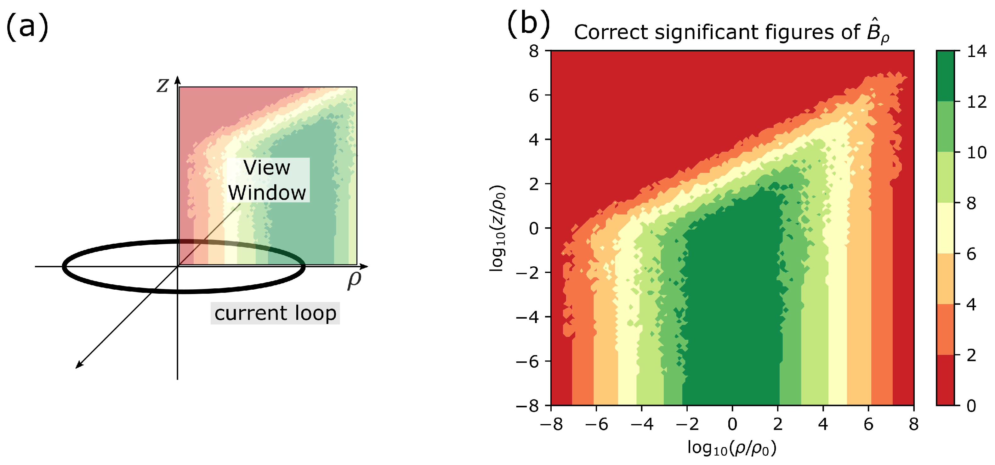
A straightforward implementation of expression (1) is numerically troublesome because catastrophic cancellation happens close to the axis, , and at large distances from the loop, . The magnitude of this phenomenon is easily underestimated. For example, evaluations of in Double floating point format give only four correct significant figures when evaluated at not very distant positions . The extent of the problem is laid out in Figure 1. There, the first quadrant in -space is depicted for an arbitrary . The other quadrants follow from the symmetry of the problem.
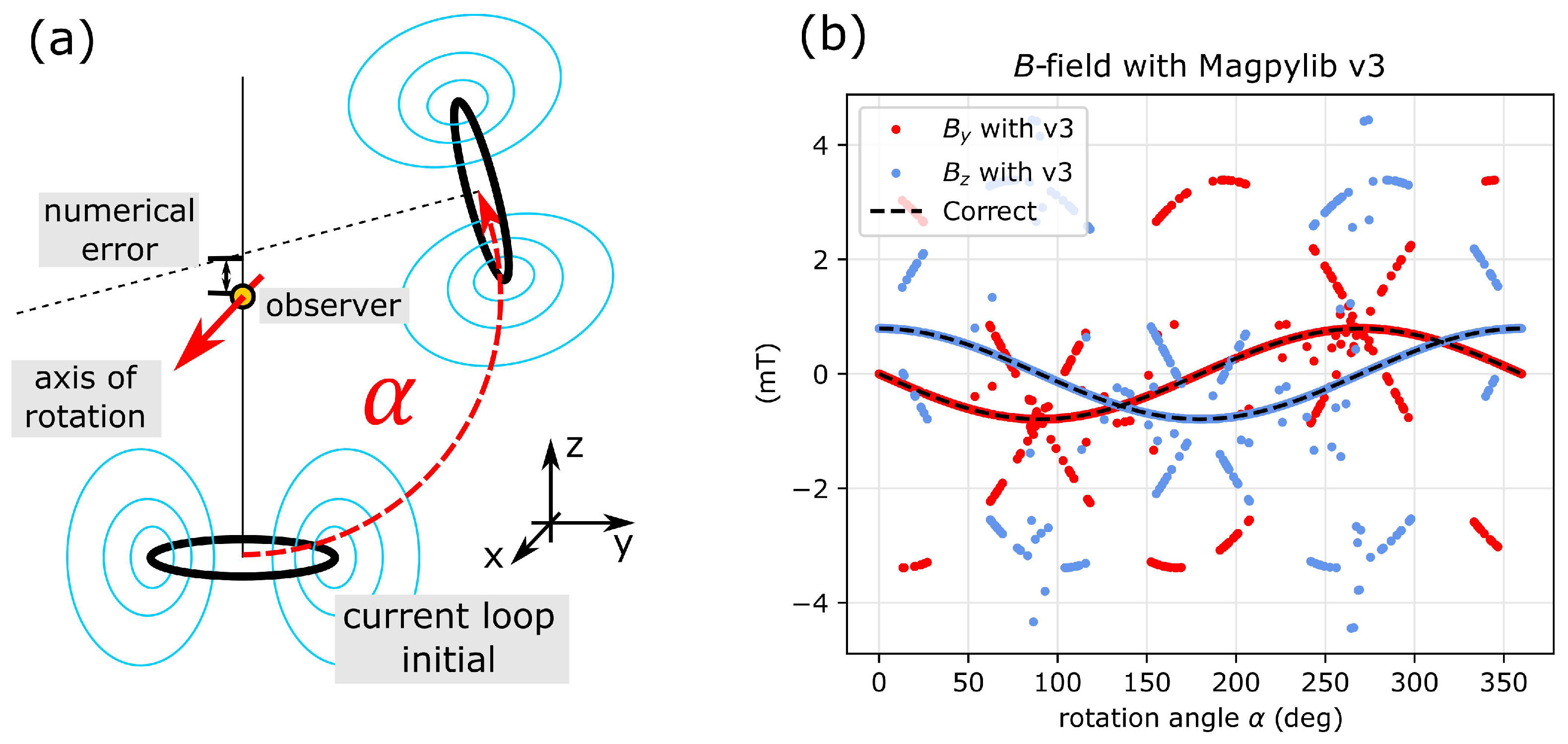
Discussions in the Magpylib [11] forum on Github underline the practical relevance of the issue. Magpylib is an open-source Python package that combines analytic solutions of permanent magnets and current problems with a geometric reference frame API. It enables users to easily compute the magnetic fields of sources at observers with arbitrary relative position and orientation. In the now outdated version 3.0.5, a numerically unstable, straightforward implementation is used for the current loop field, together with a special case for . When an unsuspecting user creates such a current loop object and rotates it about an observer located on the loop axis, see Figure 2a, the limited precision of the rotation naturally results in a misalignment between the observer and loop axis by small values of the order of the machine precision. In the reference frame of the current loop, the observer is thus moved from the stable special case, , to the numerically unstable position . The resulting bad computation is shown in Figure 2b for multiple angles ranging from 0 to 360 degrees. Complete loss of precision can be observed in many cases.
Achieving numerical stability is of critical importance. Instabilities like the one described in this work are often not visible, but can lead to erroneous computation results that are difficult to track down. In this paper, we analyze various expressions for the B-field of a current loop in terms of range of validity, precision, numerical stability and performance. Eventually, a reader can decide by himself which formulation suits his needs best.
The structure of the manuscript is as follows: In Section 2, the classical textbook expression is discussed, the origin of the problem is identified, and several expressions for the B-field are introduced and analyzed in terms of accuracy. In Section 3, all these expressions are tested in terms of computation performance. In Section 4, all results are reviewed and discussed. Finally, in Appendix A, various algorithms used in this work are provided.
2. Numerical Stability
2.1. Fundamentals and Annotation
As this paper is intended mostly for physicists and engineers, we outline a few basic concepts and annotation details common in numerical analysis, following the textbook Accuracy and Stability of Numerical Algorithms [12].
Evaluation of an expression in floating point arithmetic is denoted . A basic arithmetic operation satisfies
Here, u is the machine precision, which is for the standard 64 bit Double floating point format, which is also used in this work. In contrast to the textbook, we use the common notation that bold symbols denote vectors, and also do not distinguish between accuracy and precision.
Computed quantities wear a hat, i.e., denotes the computed value of an expression f. The absolute error of a computed quantity is defined as, . In relation to the function value, it gives the important relative error
The intuitive measure of correct significant figures of an evaluation is a flawed concept, as explained in the textbook, but is used here nonetheless by rounding the relative error. In most cases, an evaluation of experiences large relative errors about zero crossings of the function f, accompanied by a respective loss of significant figures. However, this is generally not a problem as long as the absolute error is reasonably bounded there, .
We speak of numerical stability when the relative error is small, or at zero crossings, when the absolute error is, respectively, smaller than the mean absolute function value in the vicinity of the crossing. In Double floating point format, proper implementations of analytic expressions are expected to give relative errors below to , or in the vicinity of zero-crossings, absolute errors that are at least 10–12 orders of magnitude smaller than the mean absolute function value.
When a vector field is studied, this is done componentwise with (3), or vectorwise using the Euclidean norm ,
Such a measure can also mitigate the apparent relative error problem about zero-crossings of individual components.
Rounding happens when an internal operation results in a number that has more decimal places than is provided by the used floating point arithmetic. For example, the input can be fully represented in Single (32 bit) precision, while the result of is rounded off. Rounding is by itself not a problem, since the error appears only in the last digit. The relative error according to (3) yields , which is in the expected range for Single precision with 7–8 significant digits. However, this rounding error sets the stage for numerical cancellation. Consider that a number is subtracted from the previous result. The outcome is and has only three significant figures. The resulting relative error increases to in this case. Further computation with this value must be treated with great care. Numerical cancellation happens when subtracting rounded values of equal size from each other, and can even lead to a complete loss of precision, i.e., no correct significant figures.
A power series can be assumed to be stable when implementing the sum with falling order (small terms first). The limit of precision of a series expansion is mostly a result of the chosen truncation.
In this work, all quantities are evaluated in Python v3.9.9, and making use of the standard packages Numpy v1.21.5 and Scipy v1.7.3. Many of the used implementations are reproduced in Appendix A.
2.2. The Classical Solution
The exact analytic expressions for the off-axis magnetic field of a circular current loop have been known for a long time. They can either be derived by direct integration over the current density, or by solving a boundary value problem. A few examples included in classical textbooks show expressions derived in cylindrical coordinates [5] and in spherical coordinates [13] via the vector potential. A solution via the boundary value problem is demonstrated in [14]. A detailed summary of analytic expressions for the current loop field and their derivatives in different coordinate systems is given in [15]. More recent developments show a computation through the law of Biot–Savart where the result is expressed in terms of hypergeometric functions [16]. In [17], the field of arc segments is reviewed and expressed in terms of incomplete elliptic integrals, where the special case of a complete current loop is shown to yield the classical results.
Two recent works focus on computationally efficient approximation schemes: Prantner et al. [18] use local Taylor series approximations about supporting points. This has the advantage that the resulting expressions are simple, numerically stable and fast to compute. On the other hand, the validity is limited to small regions about the supporting points, and for each new region, a new series must be constructed. A very elegant solution was proposed by Chapman et al. [19]. They make use of a binomial expansion and reduce the field to a simple series with a high level of accuracy everywhere. Their work aligns strongly with this paper, is reproduced in Section 2.6, and analyzed in terms of performance in Section 3.
Hints towards stability problems of the classical solutions are found in [20], where the authors use a series expansion to “obtain simpler expressions valid at intermediate distances”, and in [21], where various analytic representations are derived and studied. Proper numerical implementation, numerical stability and computation performance are hardly discussed in the literature beyond basic algorithms for the complete elliptic integrals and Taylor series expansions.
All works that offer exact analytic forms for the field of the current loop end up with the same expressions in cylindrical coordinates, or with expressions that are easily transformed to the following one
The loop lies in the plane of a cylindrical coordinate system , with the origin at its center. and denote radial and axial component of the B-field, respectively. Everything is expressed in dimensionless quantities, and with the loop radius , and with the vacuum permeability . The functions K and E denote the complete elliptic integrals of first and second kind, respectively, for which fast and stable algorithms exist [6,10].
The formulation is chosen through the two dimensionless quantities k and q that satisfy
While k and q can be expressed through each other, it is important that they are computed individually to avoid numerical cancellation effects. Specifically, a pure k-formulation results in additional problems about the singularity at , while a pure q-formulation adds to the main instability described in the next section.
The system is independent of the azimuth angle , so that the parameter space of interest, covering all of except the loop itself, is,
Due to the symmetry, we only study positive values of .
2.3. Numerical Stability of the Classical Solution
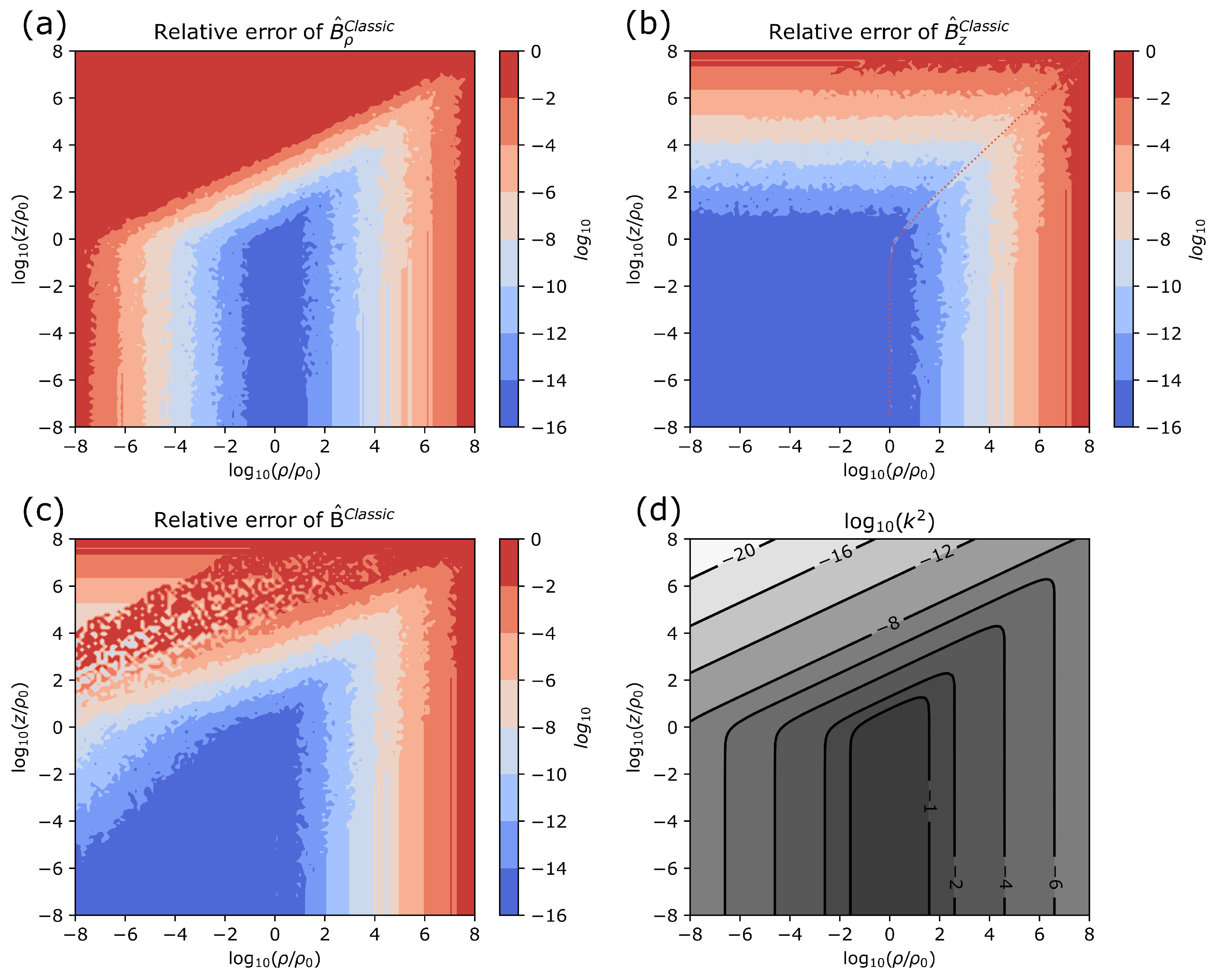
By straightforward implementation, we mean naive transfer of a function to the computer script. A code example for such an implementation of Equation (5) is provided in Appendix A.1. This implementation is component- and vectorwise numerically unstable, which can be seen from the relative errors shown in Figure 3. An increasing loss of precision with distance from the loop () can be observed in all subplots. In addition, the radial component becomes unstable towards the axis (). This instability translates partially to the vectorwise error in (c), despite the dominating amplitude of the stable . The troublesome "speckled" region in (c) is the result of the competing error between the two components. Finally, the relative error diverges naturally in a narrow band about the zero crossing of the z-component, outlined with a dotted line in (b). All error computations in this work are achieved by comparison to stable forms that are derived below.
The origin of the observed instabilities is numerical cancellation when evaluating the functions and in (5). Both functions are made up of two summands that tend to and , respectively, for , which corresponds to regions close to the axis and far from the loop, as can be seen from Figure 3d.
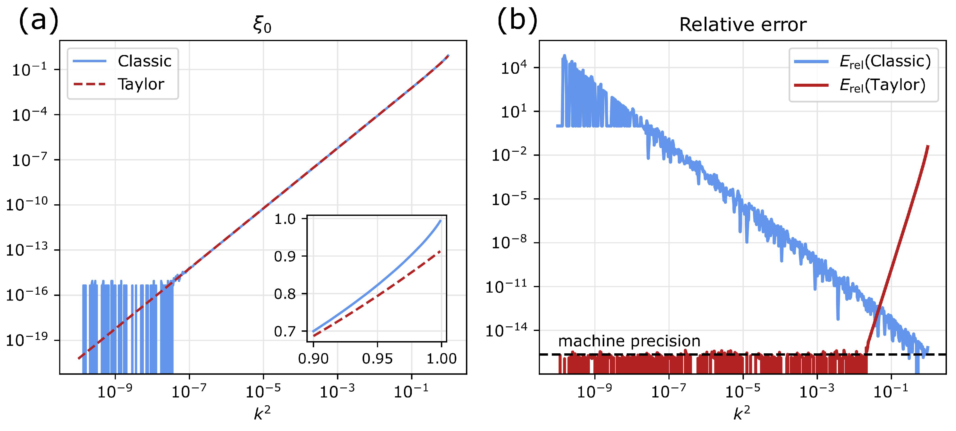
The cancellation effect is best demonstrated with the function . Figure 4a shows a straightforward implementation of , and an implementation of its Taylor series for small k including eight terms up to order . The fluctuation of with decreasing k is a result of the numerical cancellation, which ends in a complete loss of accuracy below . Loss of precision resulting from the truncation of the Taylor expansion, as k approaches 1, is made visible in the inset figure.
Relative errors of the two implementations are shown in Figure 4b. With decreasing k the straightforward implementation loses precision. Below the relative error exceeds 1 which is understood as a complete loss of precision. On the other hand, the accuracy of the Taylor series increases with decreasing k until the truncation error undercuts the machine precision. For small values of k, this Taylor series can be used as an excellent numerical reference.
All exact expressions for the magnetic field of a current loop that are provided in the literature seem to exhibit similar instabilities. This includes the tempting form in spherical coordinates [13,15]. Rearrangement of the problematic summands can partially reduce some cancellation effects, but the main problem remains.
2.4. Dipole Approximation
Dipole models are commonly used to describe the magnetic field at large distances from the sources. They are numerically stable, easy to implement and fast to compute. Specifically for current loops, dipole models are used when coupling distant coils [22], or in some geomagnetic works [23,24]. The relation between the magnetic dipole moment and the current loop parameters is . The resulting dipole field in cylindrical coordinates is given by
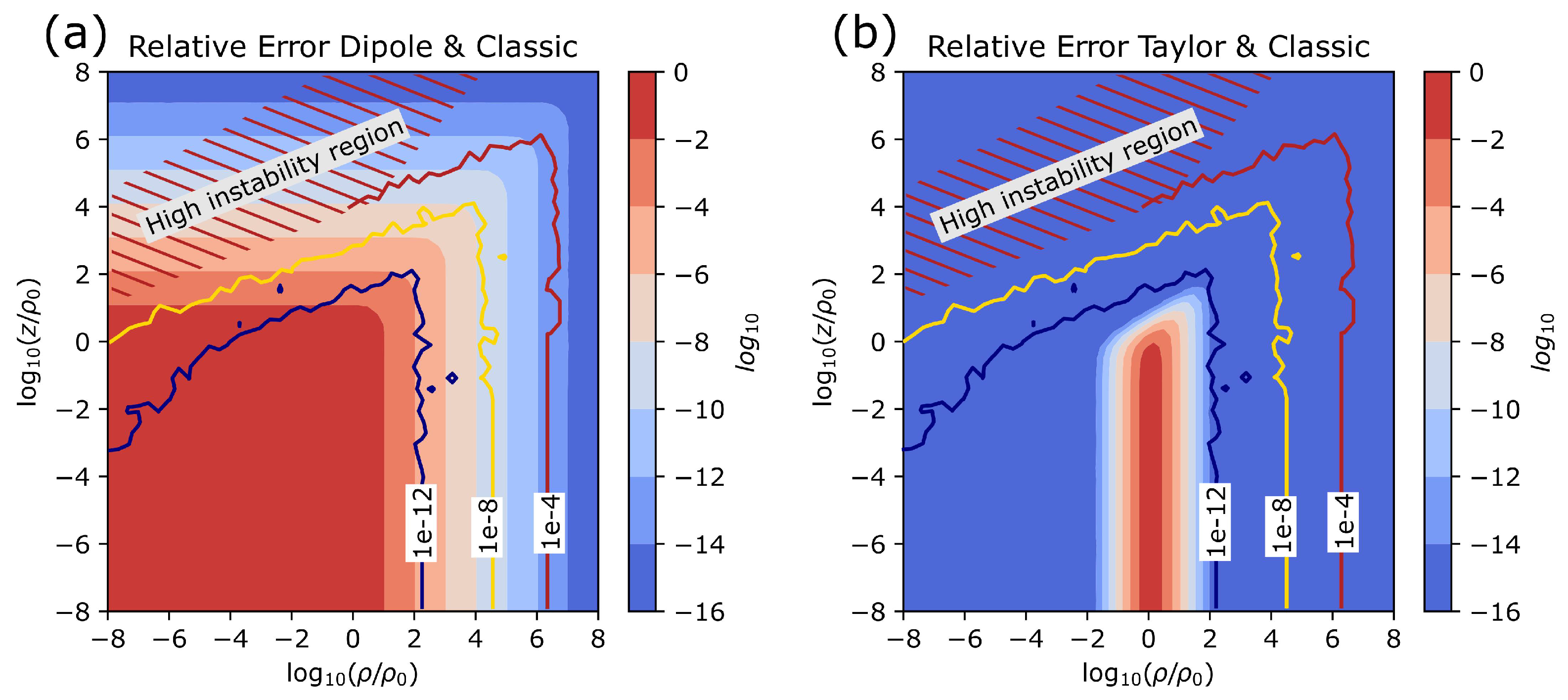
Straightforward implementations of (8) are numerically stable, so that the precision of the dipole model is limited only by the approximation error. The vectorwise relative error is shown in Figure 5a. It can be observed that the accuracy of the dipole approximation increases only slowly with distance from the loop. At , the relative error is still above . The large difference between current loop and dipole model is also noted in [20].
The colorful contour lines in the figure correspond to the vectorwise relative error of , and are taken from Figure 3c. While the dipole approximation saves the day at large distances, the figure also reveals that both computations fail to give correct results in a large region of interest close to the axis.
2.5. Taylor Approximation
In Section 2.3, it is explained that the classical textbook expressions suffer from the numerical instabilities of and for small values of k. A series expansion seems like a natural choice. Taylor approximations of (5a) and (5b) about calculate as
The vectorwise error of such a series expansion with up to order (10 terms) is shown in Figure 5b. Such an expansion with a simple cutoff criterion can be combined with the classical solution (5) to yield at least 10 significant digits everywhere.
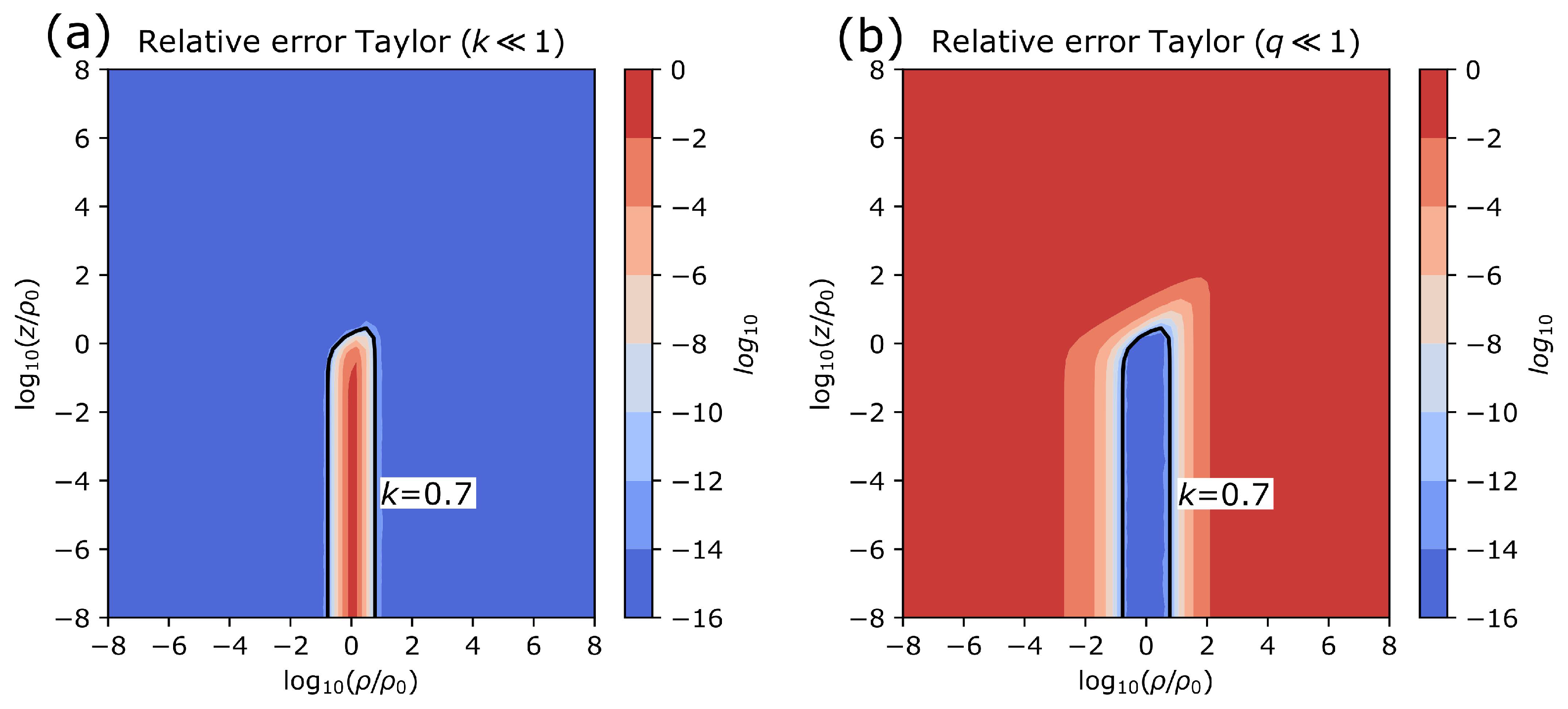
Moreover, it is possible to provide a second Taylor series about , which is accurate when the k-series fails,
Here e denotes Euler’s number. It is shown in Figure 6 that it is possible to cover all of by overlapping a k-series and a q-series. Specifically, two such series that include terms up to order and with cutoff criterion globally undercut a componentwise relative error of . The respective contour is shown in Figure 6a,b.
Proper implementations of these series are provided in Appendix A.2, together with detailed information about the series precision with respect to the chosen truncation. Computation performance is discussed in Section 3.
2.6. Binomial Expansion
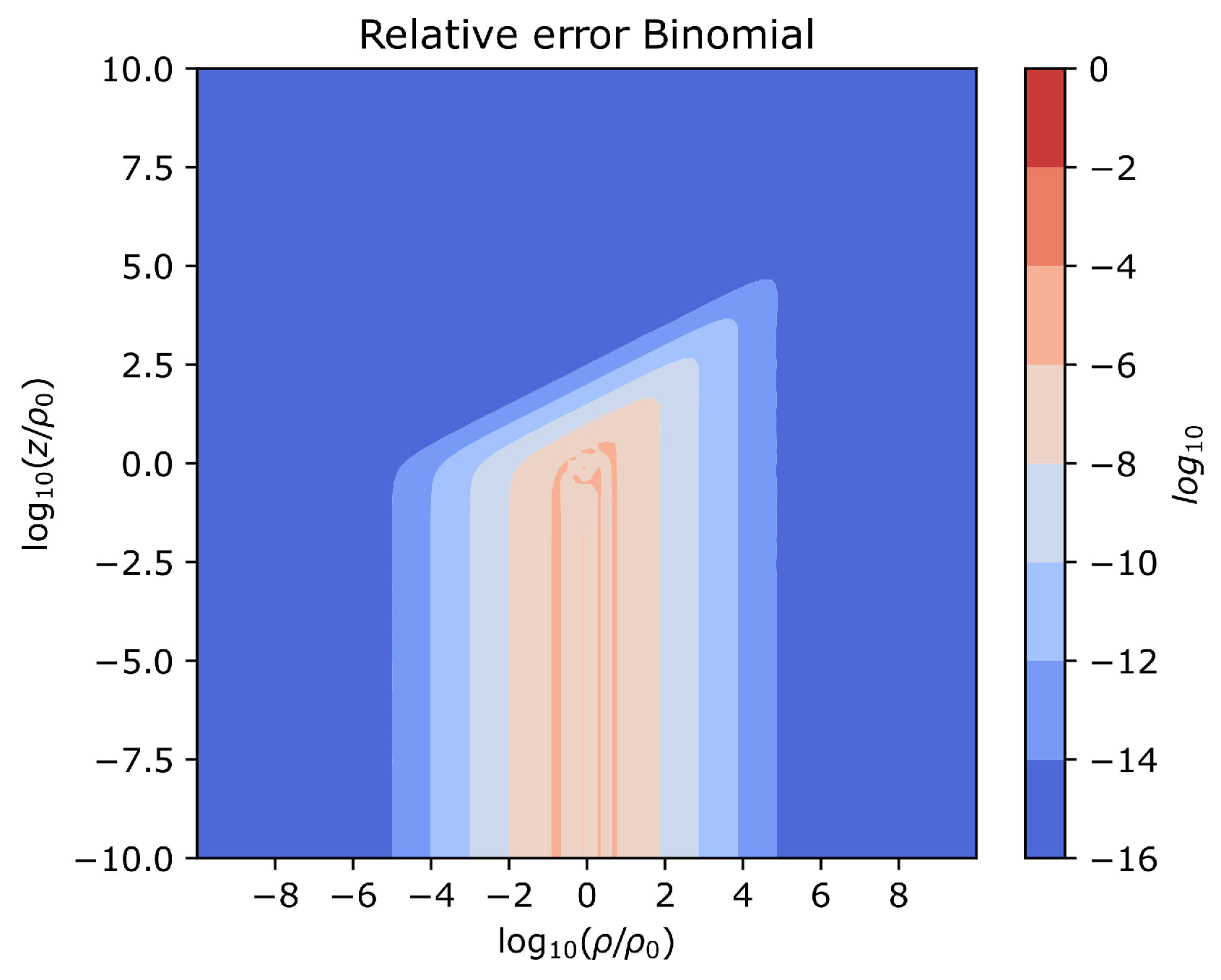
It is proposed in [19] to make use of a binomial expansion to generate the following series approximation for the B-field of a current loop,
The quantity W is closely related to ,
and the functions and coefficients for the lowest five orders are given by
The corresponding coefficients and are
Here, we have simply reproduced the results from Chapman et al. in a format that aligns with this work. Coefficient has a different sign due to a typo in the original publication.
When implementing the above expressions, great care must be taken with the functions and , as they are numerically unstable for small values of W. For this purpose, special implementations, commonly termed and , can be used. The resulting accuracy is displayed in Figure 7, and confirms the claims made in [19], that more than five significant digits are achieved everywhere with this approximation.
2.7. An Exact and Stable Representation
Bulirsch’s general complete elliptic integral [25] is defined as
An efficient algorithm exists for the computation of . Its original implementation by Bulirsch [25] is reviewed in [26] and is reproduced here in Appendix A.3. A slightly faster, but more verbose implementation by Fukushima can be found in [27]. Algorithm convergence and performance is discussed in Section 3.
It is pointed out in [28] that sums of complete elliptic integrals can be expressed in terms of ,
This identity enables us to re-express the troublesome functions and in the form of
Again, we have chosen a favorable argument representation through k and q to avoid instabilities about the singularity at and .
In principle, the transformation from E and K to eliminates the numerical cancellation problems of and . However, the implementations by Bulirsch and by Fukushima become themselves numerically unstable for small values of k when evaluating (15) and (16).
A closer look at the algorithm in Appendix A.3 reveals the problem: At first (line 7–34), a set of parameters is prepared from the input arguments, thereon (line 35–44) the solution is computed iteratively. For the input arguments in (15), it happens that line 28 becomes , which exhibits cancellation for . This problem is easily fixed by rewriting the expression as in that line. Similar problems, which can be solved by algebraic transformations in the first part of the algorithm, happen also when computing in (16).
In Appendix A.4 and Appendix A.5, we show modified algorithms, termed and for computing and , respectively, that are stable and fast. For improved performance, the first part of Bulirsch’s original algorithm is shortened down by assigning all parameters their respective values, and the improvements proposed by Fukushima [27] are adapted. Comparisons to overlapping Taylor series expansions, introduced in Section 2.5 confirm the global numerical stability of the two algorithms.
As all other terms in (5) are numerically stable, the following expressions will give the components of the B-field of a current loop with machine precision everywhere,
2.8. Loss of Precision at Sign Change
The z-component of the B-field exhibits a sign change when passing from small to large values of . In (17b), the sign change is revealed by the following relation:
Both functions E and are positive. Towards the coordinate axis, the first term dominates, while for large values of , the second term does. The zero-crossing in-between corresponds to the change in sign.
The relative error of the z-component naturally diverges around the zero-crossing. As explained in Section 2.1, we do not speak of numerical instability in this case, however, a loss of significant digits of the z-component still occurs. How fast the loss of significant digits occurs depends on the gradient of the field. In this case, a helpful criterion is found empirically
which corresponds only to a very narrow band about the crossing.
3. Performance
Analytic solutions are mostly used for their computation efficiency, so that the performance of the proposed algorithms is critical. For a performance comparison on equal footing, all algorithms are implemented for scalar inputs in native Python, and making use of the standard package. This means that only sequential execution is considered, the potential for code vectorization is not analyzed here. Algorithms for the complete elliptic integrals, that can also be found in the Scipy library, have been reproduced. All tests were run on CentOS Linux 7.9.2009 operating system on a AMD EPYC 7513 2.6 GHz CPU architecture with 32 cores.
The performance test is designed as follows: Each B-field expression is evaluated for input parameters . This is repeated for a set of 200 different points, that all correspond to a similar value of k. The points are equally distributed on the respective contour lines that are shown in Figure 3d. This procedure is repeated in a loop 1000 times. For each value of k, every expression is thus evaluated 200,000 times. The order of evaluation is mixed up by design, to avoid distortions from computation performance spikes resulting from Python garbage collection and hardware issues. For each k, the computation times of every tested expression are summed up.
The results of this test are shown in Figure 8a for different values of . Computation times are displayed with respect to the fastest one, which is always the dipole expression. Most algorithms evaluate the same expression independent of k, and show similar timings for all inputs. The proposed stable algorithm is of an iterative nature, and requires less iterations for smaller values of k. The steps from four iterations close to the loop filament down to zero iterations are clearly visible in the figure. The binomial approximation exhibits a step at about , which results from the special implementation of that was used here. This function is not available in Python , and makes use of a 4-term power series for small W.
In Figure 8b, we show the maximal vectorwise relative computation errors of the different methods. Interestingly, convergence and divergence of most methods can be observed well as functions of . For the dipole approximation only positions with on the contour lines are included, because it does not converge close to the origin. The stable solution is not visible in this figure, because it is used as a reference. It has machine precision everywhere.
The combination of the two figures enables users to choose the scheme that is most suitable for their purpose. When only computation time and accuracy are taken as measures, Figure 8 shows that the proposed method is extremely competitive. The only solutions that are faster and have similar precision are the Taylor k-series and the dipole approximation, both with limited validity. However, in many cases users might not require machine precision, and can be compelled by the simple analytic expressions offered by the approximation schemes, which also enable effortless computation of the derivatives.
4. Discussion and Conclusions
We have studied straightforward implementations of the textbook expressions for the B-field of a current loop (5), and have found that these commonly used forms are numerically troublesome at large distances from the loop and close to the axis. The computationally fast dipole approximation (8) appears to be an unsatisfactory option, as it converges very slowly and solves the problem only at large distances. Instead, a well-chosen Taylor series approximation (9) with a simple cutoff criterion can mitigate the instability globally. It is also possible to cover all of with two overlapping Taylor series (9) and (10). However, to achieve good precision, the series must include a high order, which makes them computationally slow. A recently proposed binomial expansion (11) offers simple expressions and excellent computation performance. The only downside is the limited accuracy (more than five significant figures) in the vicinity of the loop. The real advancement of this paper is a novel, exact, numerically stable representation in terms of modified Bulirsch functions (17). Implementations based thereon offer machine precision everywhere and much faster computation times than the classical solution.
For achieving numerical stability, series approximations are always an interesting option. However, there are several arguments that speak for the proposed approach: The approximation error of the series is a result of truncation and cannot improve unless more terms are included, while the machine precision limit of the proposed algorithm depends only on the chosen floating point arithmetic. This means that a 128 bit implementation will give twice as many correct significant figures as a 64 bit implementation when using , while the series will not improve. Of course, this comes at the cost of more automatic iterations. Secondly, most approximations have a limited region of validity which requires cut-off criteria and treating multiple cases. This is problematic because in addition to programming complexity, case splitting hinders code vectorization, which can be a serious performance issue. Moreover, a -based implementation can further reduce computation time by combining the time consuming iterative parts of both field components in a single vectorized operation.
The biggest advantage of the approximation schemes is their simple form, which makes it easy to find analytic expressions for their derivatives. While it is also possible to determine derivatives of the proposed expressions, making them numerically stable seems quite laborious.
Similar stability problems of analytic forms can be found throughout the literature when systems of cylindrical symmetry are involved. Specific examples are expressions found for the axially magnetized cylinder [26], the diametrically magnetized cylinder [29], and homogeneously magnetized ring segments [30]. It is very likely that the arc solutions [17] also suffer from this problem. A similar treatment should be attempted for the extremely useful expressions in these works.
Finally, we are happy to announce that the proposed implementation of the magnetic field of a current loop, based on the and algorithms, was adopted into the open-access Python package Magpylib version 4.2.0 and is already available to the general public.
Author Contributions
Conceptualization, methodology, validation and investigation were performed by M.O. and P.L.; original draft preparation, visualization, administration and funding were conducted by M.O.; writing, review and editing, formal analysis were done by P.L. and F.S. All authors have read and agreed to the published version of the manuscript.
Funding
This project has been supported by the COMET K1 centre ASSIC Austrian Smart Systems Integration 100 Research Center.
Institutional Review Board Statement
Not applicable.
Informed Consent Statement
Not applicable.
Data Availability Statement
Not applicable.
Acknowledgments
This project has been supported by the COMET K1 centre ASSIC Austrian Smart Systems Integration 100 Research Center. The COMET—Competence Centers for Excellent Technologies—Program is supported by BMVIT, 101 BMDW and the federal provinces of Carinthia and Styria. Feedback and discussions with Christoph Ortner on numerical analysis were highly appreciated. Thanks to Github users @fwessel and @Blue-Spartan for pointing out numerical stability issues in the Magpylib computations. Special thanks to Alexandre Boisellet for his support of the Magpylib project.
Conflicts of Interest
The funders had no role in the design of the study; in the collection, analyses, or interpretation of data; in the writing of the manuscript; or in the decision to publish the results.
Appendix A. Algorithms
All algorithms in this section are written in Python 3.9. They are presented in a scalar form for readability.
Appendix A.1. Straightforward Implementation
The following code shows a naive implementation of the classical expressions (5) of the B-field of a current loop in cylindrical coordinates.

Appendix A.2. Taylor Series Implementations
The following code is an implementation of the Taylor series expansion (9a) with orders up to .

The following code is an implementation of the Taylor series expansion (10a) with orders up to .

The following code is an implementation of the Taylor series expansion (9b) with orders up to .

The following code is an implementation of the Taylor series expansion (10b) with orders up to .


In most cases, the 30 provided terms will not be necessary. A relation between the number of terms included and precision of the Taylor series is shown in Table A1. The table gives values of k below (k-series) or above (q-series) which a series has a precision below the indicated number of significant figures when the indicated order is included in the sum. For example, an implementation of Br_taylor_k that includes up to order has at least 8 digits of precision when . An implementation of Br_taylor_q that includes up to order has at least 10 digits of precision when .

Table A1.
Precision of various Taylor implementations in relation to the number of terms included in the respective sums.
Table A1.
Precision of various Taylor implementations in relation to the number of terms included in the respective sums.
| Br_taylor_k ( value) | Br_taylor_q ( value) | ||||||||||
|---|---|---|---|---|---|---|---|---|---|---|---|
| sig.figs | k-order included in series | sig.figs | q-order included in series | ||||||||
| 21 | 31 | 41 | 51 | 61 | 20 | 30 | 40 | 50 | 60 | ||
| 8 | 0.46 | 0.62 | 0.71 | 0.77 | 0.81 | 8 | 0.77 | 0.67 | 0.60 | 0.55 | 0.50 |
| 10 | 0.35 | 0.53 | 0.63 | 0.70 | 0.75 | 10 | 0.85 | 0.76 | 0.69 | 0.63 | 0.58 |
| 12 | 0.27 | 0.45 | 0.56 | 0.64 | 0.69 | 12 | 0.90 | 0.82 | 0.75 | 0.70 | 0.65 |
| Bz_taylor_k ( value) | Bz_taylor_q ( value) | ||||||||||
| sig.figs | k-order included in series | sig.figs | q-order included in series | ||||||||
| 21 | 31 | 41 | 51 | 61 | 20 | 30 | 40 | 50 | 60 | ||
| 8 | 0.43 | 0.59 | 0.68 | 0.74 | 0.78 | 8 | 0.86 | 0.76 | 0.70 | 0.64 | 0.59 |
| 10 | 0.33 | 0.50 | 0.61 | 0.68 | 0.73 | 10 | 0.91 | 0.83 | 0.76 | 0.71 | 0.66 |
| 12 | 0.26 | 0.43 | 0.54 | 0.62 | 0.68 | 12 | 0.94 | 0.87 | 0.81 | 0.76 | 0.72 |
Appendix A.3. Original Implementation of Bulirsch’s cel Algorithm
The original implementation of Bulirsch’s algorithm [25] is reproduced here. This implementation is also found in the first edition of the popular Numerical Recipes [31] and is commented on in [26]. Advantages of the algorithm over representations in terms of Carlson’s functions are discussed in [32]. A slightly faster implementation by Fukushima is found in [27].

Appendix A.4. Implementation of cel *
Here, we show a modification of Bulirsch’s algorithm for computing the function , described in Section 2.7. Input arguments are and . A vectorized version of this algorithm is provided by the open-source library Magpylib [11].

Appendix A.5. Implementation of cel **
Here, we show a modification of Bulirsch’s algorithm for computing the function , described in Section 2.7. Input arguments are , and . A vectorized version of this algorithm is provided by the open-source library Magpylib [11].

References
- Madenci, E.; Guven, I. The Finite Element Method and Applications in Engineering Using ANSYS®; Springer: Berlin/Heidelberg, Germany, 2015. [Google Scholar]
- Pryor, R.W. Multiphysics Modeling Using COMSOL®: A First Principles Approach; Jones & Bartlett Publishers: Burlington, MA, USA, 2009. [Google Scholar]
- Alnæs, M.; Blechta, J.; Hake, J.; Johansson, A.; Kehlet, B.; Logg, A.; Richardson, C.; Ring, J.; Rognes, M.E.; Wells, G.N. The FEniCS project version 1.5. Arch. Numer. Softw. 2015, 3, 9–23. [Google Scholar]
- Schöberl, J. C++ 11 Implementation of Finite Elements in NGSolve; Institute for Analysis and Scientific Computing, Vienna University of Technology: Vienna, Austria, 2014; Volume 30. [Google Scholar]
- Smythe, W.B. Static and Dynamic Electricity; Hemisphere Publishing: New York, NY, USA, 1988. [Google Scholar]
- Moshier, S.L.B. Methods and Programs for Mathematical Functions; Ellis Horwood Ltd Publisher: Chichester, UK, 1989. [Google Scholar]
- ALGLIB. Available online: https://www.alglib.net/download.php (accessed on 9 June 2022).
- Wolfram, S. The Mathematica Book; Wolfram Research, Inc.: Champaign, IL, USA, 2003; Volume 1. [Google Scholar]
- MATLAB. Version 7.10.0 (R2010a); The MathWorks Inc.: Natick, MA, USA, 2010. [Google Scholar]
- Virtanen, P.; Gommers, R.; Oliphant, T.E.; Haberland, M.; Reddy, T.; Cournapeau, D.; Burovski, E.; Peterson, P.; Weckesser, W.; Bright, J.; et al. SciPy 1.0: Fundamental algorithms for scientific computing in Python. Nat. Methods 2020, 17, 261–272. [Google Scholar] [CrossRef] [PubMed] [Green Version]
- Ortner, M.; Bandeira, L.G.C. Magpylib: A free Python package for magnetic field computation. SoftwareX 2020, 11, 100466. [Google Scholar] [CrossRef]
- Higham, N.J. Accuracy and Stability of Numerical Algorithms; SIAM: Philadelphia, PA, USA, 2002. [Google Scholar]
- Jackson, J.D. Classical electrodynamics. Am. J. Phys. 1999, 67, 841. [Google Scholar] [CrossRef]
- Ortner, M.; Filipitsch, B. Feedback of Eddy Currents in Layered Materials for Magnetic Speed Sensing. IEEE Trans. Magn. 2017, 53, 1–11. [Google Scholar] [CrossRef]
- Simpson, J.C.; Lane, J.E.; Immer, C.D.; Youngquist, R.C. Simple Analytic Expressions for the Magnetic Field of a Circular Current Loop; Technical Report; NASA, Kennedy Space Center: Merritt Island, FL, USA, 2001. [Google Scholar]
- Behtouei, M.; Faillace, L.; Spataro, B.; Variola, A.; Migliorati, M. A novel exact analytical expression for the magnetic field of a solenoid. Waves Random Complex Media 2020, 32, 1977–1991. [Google Scholar] [CrossRef]
- González, M.A.; Cárdenas, D.E. Analytical Expressions for the Magnetic Field Generated by a Circular Arc Filament Carrying a Direct Current. IEEE Access 2020, 9, 7483–7495. [Google Scholar] [CrossRef]
- Prantner, M.; Parspour, N. Analytic multi Taylor approximation (MTA) for the magnetic field of a filamentary circular current loop. J. Magn. Magn. Mater. 2021, 517, 167365. [Google Scholar] [CrossRef]
- Chapman, G.H.; Carleton, D.E.; Sahota, D.G. Current Loop Off Axis Field Approximations with Excellent Accuracy and Low Computational Cost. IEEE Trans. Magn. 2022, 58, 1–6. [Google Scholar] [CrossRef]
- Seleznyova, K.; Strugatsky, M.; Kliava, J. Modelling the magnetic dipole. Eur. J. Phys. 2016, 37, 025203. [Google Scholar] [CrossRef]
- Schill, R.A. General relation for the vector magnetic field of a circular current loop: A closer look. IEEE Trans. Magn. 2003, 39, 961–967. [Google Scholar] [CrossRef]
- Urzhumov, Y.; Smith, D.R. Metamaterial-enhanced coupling between magnetic dipoles for efficient wireless power transfer. Phys. Rev. B 2011, 83, 205114. [Google Scholar] [CrossRef]
- Rong, Z.; Wei, Y.; Klinger, L.; Yamauchi, M.; Xu, W.; Kong, D.; Cui, J.; Shen, C.; Yang, Y.; Zhu, R.; et al. A New Technique to Diagnose the Geomagnetic Field Based on a Single Circular Current Loop Model. J. Geophys. Res. Solid Earth 2021, 126, e2021JB022778. [Google Scholar] [CrossRef]
- Alldredge, L.R. Circular current loops, magnetic dipoles and spherical harmonic analyses. J. Geomagn. Geoelectr. 1980, 32, 357–364. [Google Scholar] [CrossRef] [Green Version]
- Bulirsch, R. Numerical calculation of elliptic integrals and elliptic functions. III. Numer. Math. 1969, 13, 305–315. [Google Scholar] [CrossRef]
- Derby, N.; Olbert, S. Cylindrical magnets and ideal solenoids. Am. J. Phys. 2010, 78, 229–235. [Google Scholar] [CrossRef] [Green Version]
- Fukushima, T.; Kopeikin, S. Elliptic functions and elliptic integrals for celestial mechanics and dynamical astronomy. Front. Relativ. Celest. Mech. 2014, 2, 189–228. [Google Scholar]
- Fukushima, T.; Ishizaki, H. Numerical computation of incomplete elliptic integrals of a general form. Celest. Mech. Dyn. Astron. 1994, 59, 237–251. [Google Scholar] [CrossRef]
- Caciagli, A.; Baars, R.J.; Philipse, A.P.; Kuipers, B.W. Exact expression for the magnetic field of a finite cylinder with arbitrary uniform magnetization. J. Magn. Magn. Mater. 2018, 456, 423–432. [Google Scholar] [CrossRef]
- Slanovc, F.; Ortner, M.; Moridi, M.; Abert, C.; Suess, D. Full analytical solution for the magnetic field of uniformly magnetized cylinder tiles. J. Magn. Magn. Mater. 2022, 559, 169482. [Google Scholar] [CrossRef]
- Press, W.H.; Teukolsky, S.A.; Vetterling, W.T.; Flannery, B.P. Numerical Recipes 3rd Edition: The Art of Scientific Computing; Cambridge University Press: Cambridge, UK, 2007. [Google Scholar]
- Reinsch, K.D.; Raab, W. Elliptic Integrals of the First and Second Kind—Comparison of Bulirsch’s and Carlson’s Algorithms for Numerical Calculation. In Special Functions; World Scientific: Singapore, 2000; pp. 293–308. [Google Scholar]
Figure 1.
(a) Sketch of a current loop and the observed first quadrant. (b) The number of correct significant figures of a straightforward implementation of the textbook expression for the radial component of the B-field of a current loop on a log–log scale.
Figure 1.
(a) Sketch of a current loop and the observed first quadrant. (b) The number of correct significant figures of a straightforward implementation of the textbook expression for the radial component of the B-field of a current loop on a log–log scale.

Figure 2.
(a) Sketch of typical current loop positioning with the package Magpylib. (b) Demonstrating the relevance of the numerical instability, which becomes visible when a current loop rotates about an observer.
Figure 2.
(a) Sketch of typical current loop positioning with the package Magpylib. (b) Demonstrating the relevance of the numerical instability, which becomes visible when a current loop rotates about an observer.

Figure 3.
Relative error of a straightforward implementation of the textbook expressions for the B-field of a current loop. (a) Radial and (b) axial components, as well as (c) vectorwise analysis reveal a high level of numerical instability. (d) The relation between the cylindrical coordinates and the important quantity k.

Figure 4.
(a) Two different implementations of the function and (b) the relative difference when comparing them to each other.
Figure 4.
(a) Two different implementations of the function and (b) the relative difference when comparing them to each other.

Figure 5.
Vectorwise relative error of the dipole approximation (a) and a Taylor approximation (b) of the B-field of a current loop. The colored contour lines show the numerical error from a straightforward implementation of the classical textbook expressions.
Figure 5.
Vectorwise relative error of the dipole approximation (a) and a Taylor approximation (b) of the B-field of a current loop. The colored contour lines show the numerical error from a straightforward implementation of the classical textbook expressions.

Figure 6.
Vectorwise relative error of Taylor approximations of the B-field of a current loop. (a) Expansion for small k. (b) Expansion for small q.
Figure 6.
Vectorwise relative error of Taylor approximations of the B-field of a current loop. (a) Expansion for small k. (b) Expansion for small q.

Figure 7.
Vectorwise relative error of the binomial expansion for the B-field of a current loop.

Figure 8.
(a) Computation times of various methods with respect to the fastest one (dipole) as a function of . (b) The respective vectorwise relative errors.
Figure 8.
(a) Computation times of various methods with respect to the fastest one (dipole) as a function of . (b) The respective vectorwise relative errors.

Disclaimer/Publisher’s Note: The statements, opinions and data contained in all publications are solely those of the individual author(s) and contributor(s) and not of MDPI and/or the editor(s). MDPI and/or the editor(s) disclaim responsibility for any injury to people or property resulting from any ideas, methods, instructions or products referred to in the content. |
© 2022 by the authors. Licensee MDPI, Basel, Switzerland. This article is an open access article distributed under the terms and conditions of the Creative Commons Attribution (CC BY) license (https://creativecommons.org/licenses/by/4.0/).
Share and Cite
MDPI and ACS Style
Ortner, M.; Leitner, P.; Slanovc, F. Numerically Stable and Computationally Efficient Expression for the Magnetic Field of a Current Loop. Magnetism 2023, 3, 11-31. https://doi.org/10.3390/magnetism3010002
AMA Style
Ortner M, Leitner P, Slanovc F. Numerically Stable and Computationally Efficient Expression for the Magnetic Field of a Current Loop. Magnetism. 2023; 3(1):11-31. https://doi.org/10.3390/magnetism3010002
Chicago/Turabian StyleOrtner, Michael, Peter Leitner, and Florian Slanovc. 2023. "Numerically Stable and Computationally Efficient Expression for the Magnetic Field of a Current Loop" Magnetism 3, no. 1: 11-31. https://doi.org/10.3390/magnetism3010002