Deep Learning for Concrete Crack Detection and Measurement

Abstract

Concrete structures inevitably experience cracking, which is a common form of damage. If cracks are left undetected and allowed to worsen, catastrophic failures, with costly implications for human life and the economy, can occur. Traditional image processing techniques for crack detection and measurement have several limitations, which include complex parameter selection and restriction to measuring cracks in pixels, rather than more practical units of millimetres. This paper presents a three-stage approach that utilises deep learning and image processing for crack classification, segmentation and measurement. In the first two stages, custom CNN and U-Net models were employed for crack classification and segmentation. The final stage involved measuring crack width in millimetres by using a novel laser calibration method. The classification and segmentation models achieved 99.22% and 96.54% accuracy, respectively, while the mean absolute error observed for crack width measurement was 0.16 mm. The results demonstrate the adequacy of the developed crack detection and measurement method, and shows the developed deep learning and laser calibration method promotes safer, quicker inspections that are less prone to human error. The method’s ability to measure cracks in millimetres provides a more insightful assessment of structural damage, which is, in comparison to traditional pixel-based measurement methods, a significant improvement for practical field applications.

1. Introduction

A significant portion of existing civil infrastructure, such as bridges, buildings and dams, are constructed with concrete. These structures inevitably experience varying levels of deterioration and damage throughout their service life, which can arise due to a range of factors, such as ageing, increased traffic loads, accidental collisions and extreme weather conditions [1,2]. Damage is defined as material or geometric changes that occur to the material of structure [3,4]. Cracks are often the earliest indication of damage in concrete structures [5,6], and undetected cracks can worsen over time, leading to reduced structural integrity and potentially catastrophic failures, resulting in injury, loss of life and huge economic costs [7,8]. The width of a crack typically indicates the severity of damage. One of the oldest methods for detecting the presence of concrete cracks and measuring crack width, is visual inspection, where crack width is typically measured manually by using tools and instruments such as crack gauges and vernier calipers. Visual inspection and manual crack measurement are effective, but they have drawbacks, including being subjective, time consuming and susceptible to human error.

These shortcomings have been overcome by employing modern technology to perform crack inspection and measurement. Digital imaging devices coupled with image processing algorithms are widely used for crack detection and measurement because they are non-destructive. Typical image processing algorithms for image-based concrete crack detection include thresholding [9,10,11], edge detection [12,13] and binarization [14,15,16]. Morphological features, such as thinning, closing, opening, erosion and dilation, have also been commonly used to improve the results of image processing algorithms [5,16,17]. Crack detection using image processing has produced satisfactory results; however, its accuracy is, due to the need for manual parameter selection, limited by the user’s expertise. In addition to being a tedious process, image processing has low generalisation capabilities, which is because factors such as lighting conditions and image quality can affect the performance of manually selected parameters that might have previously worked perfectly under different image conditions.

Deep learning (DL) has emerged as the preferred method for concrete crack detection because of its autonomous crack detection capabilities. Early DL works focused on performing automatic classification of images, whether through binary classification or multi-class classification. Binary classification has been successfully applied to classify images as cracked or uncracked [18,19], including by Liu and Yeoh [20], who performed binary classification by using the VGG16 CNN model to classify the type of cracks, as either structural cracks or non-structural cracks. Multi-class classification has also been used to classify cracks based on their characteristics. Uwanuakwa et al. [21] used DL to classify the type/cause of cracks as vertical, diagonal, shrinkage, efflorescence, alkali-silica reaction or corrosion cracks; And Gao and Mosalam [22] used multi-class classification to classify the level and type of damage in concrete structures.

Classification using DL is an effective way of determining the presence of cracks in images. However, the method falls short in providing sufficient details that allow for detailed crack characterisation, such as crack width measurement. In order to achieve image-based crack width measurement, it is essential to obtain a segmented binary crack mask through segmentation: a binary crack mask typically represents a crack with white pixels, and sets it against a background with black pixels. The white pixels are then measured to determine the crack width.

DL is, when compared to conventional image processing techniques, seen to offer a quicker and more scalable and generalisable approach to crack segmentation. A well-trained DL segmentation model is capable of automatically segmenting cracks, regardless of factors such as lighting conditions and image quality. Most segmentation models typically consist of an encoder and decoder block. The encoder block is typically a CNN classification model. The U-Net [23] architecture, which was first introduced to assist the segmentation of medical images, has been widely adopted for crack segmentation [24,25,26]. Mirzazade et al. [26] first classified cracks using the Inception V3 CNN and then proceeded to segment the classified cracks by using the U-Net and SegNet model. Zhao et al. [27] performed crack segmentation by using a distinctive feature pyramid network (Crack-FPN), and compared the performance of Crack-FPN against U-Net, U-Net++ and automatic thresholding techniques. Fully Convolutional Networks (FCNs) have also been employed to address the crack segmentation problem [17,28,29,30,31]. Other DL networks architectures have also been used for automatic crack segmentation. For example, Kang et al. [32] used a hybrid Faster R-CNN and modified TuFF algorithm, and Yu et al. [33] proposed a custom segmentation model, Cracklab, which was a modification of DeepLabv3+ [34].

In order to fully exploit automatic crack segmentation by using DL, it is necessary to use the segmented crack masks to measure the crack width of cracks in images. The majority of studies used crack masks obtained by segmentation, and used image processing to measure concrete crack width in pixels. Kim et al. [16] measured concrete crack width in pixels by using binarisation.; Ioli et al. [14] used the medial axis transform to measure crack width on crack masks that were obtained by using the Canny edge detection image processing algorithm [12]; Yang et al. [17] used medial axis transform to measure crack width in pixels after performing skeletonization; and Mishra et al. [35] measured crack width in pixels by first measuring the length of the crack and the area of the segmented crack, before calculating average crack width by dividing the area of the crack by the length of the crack.

Although many studies have successfully measured concrete crack width by using pixels, this unit of measurement remains a significant limitation: this is because determining the width of concrete cracks in pixels does not provide practical information for field applications, as the severity of concrete crack width is better understood in millimetres. Some studies [36,37,38,39,40,41] have found ways to measure concrete crack width in millimetres by devising methods to carry out pixel to millimetre conversion. However, Nyathi et al. [5] found that these methods require knowledge of key parameters that may not always be readily available, such as focal length, camera resolution, number of pixels along the long side of image sensor, etc. Other methods used physical markers attached to the measuring surface to convert pixels to millimetres. Although the conversion of pixels to millimetres was successfully achieved, a new challenge of imposed safety risks was introduced, especially in hard-to-reach areas. To overcome these challenges, we previously developed a novel laser calibration method [5] for converting pixels to millimetres by using a laser beam. While the method performed well, achieving a mean absolute error of 0.26 mm, it was limited, both by the use of image processing techniques for crack segmentation and the angle at which images were captured. Therefore, the aim of this paper is to enhance the performance of our previous work [5] by proposing a three-stage approach that incorporates DL for crack classification, segmentation and measurement. This has been accomplished by the:

-

development of an automatic image-based crack classification method that uses a CNN model to determine if cracks are present in an image, and does this by classifying them as cracked or not cracked;

-

development of a crack segmentation model, which is designed to segment the cracks identified in the images and classified as cracked;

-

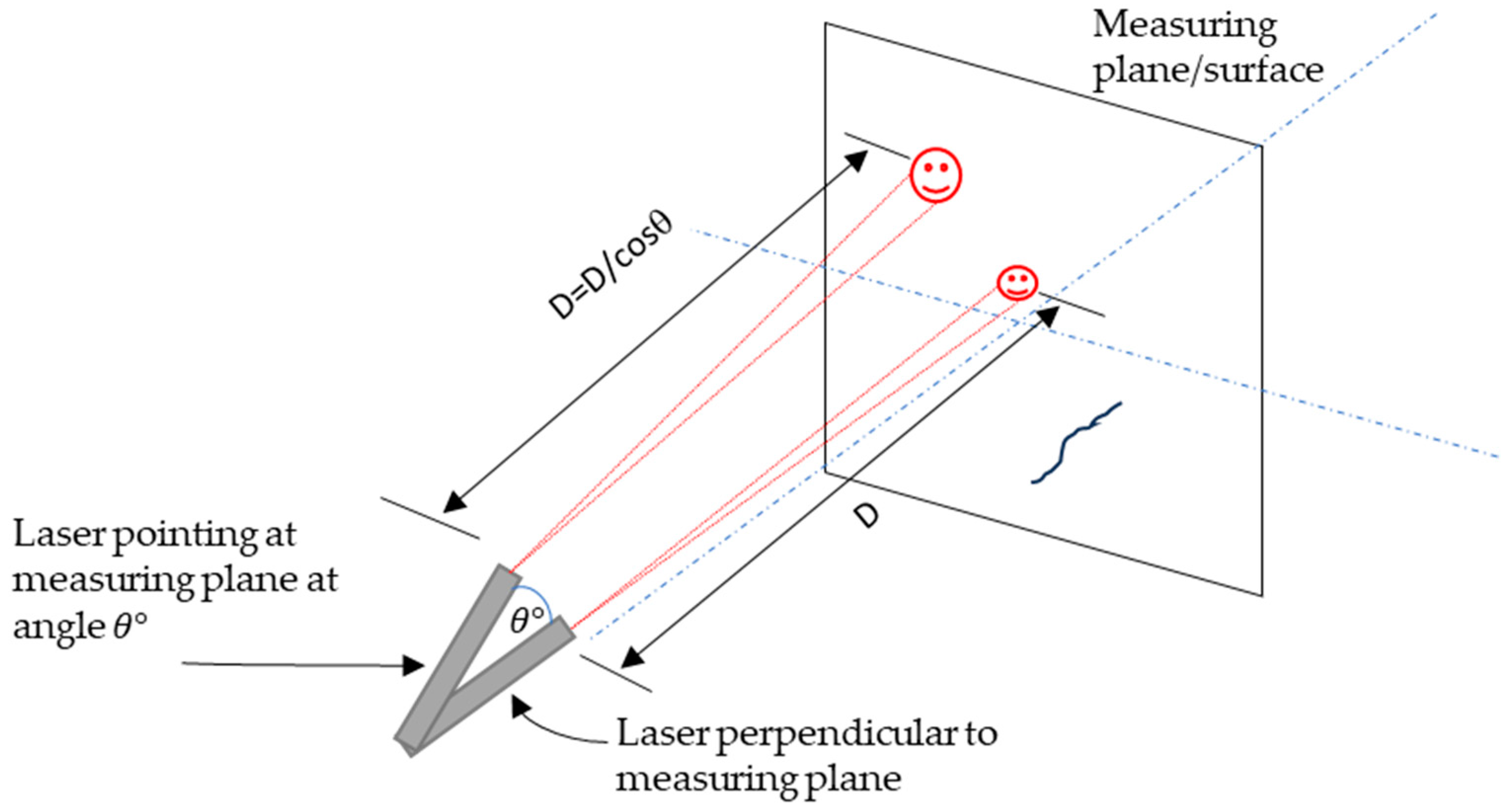
crack width measurement of the segmented cracks masks in millimetres, which is achieved by using improved laser calibration;

-

evaluation and validation of the developed method, which is achieved by comparing the measured crack widths which are obtained through deep learning and image processing against manual measurements.

The rest of the article is structured as follows: Section 2 presents the methodology used to develop DL algorithms for crack classification and segmentation. This section also covers the approach used in data collection, and the dataset generation used to train the deep learning models. Section 3 presents the classification, segmentation and crack width measurement results and discusses their implications. The paper concludes with Section 4, which makes concluding remarks about the work conducted and highlights the paper’s contribution to knowledge.

2. Materials and Methods

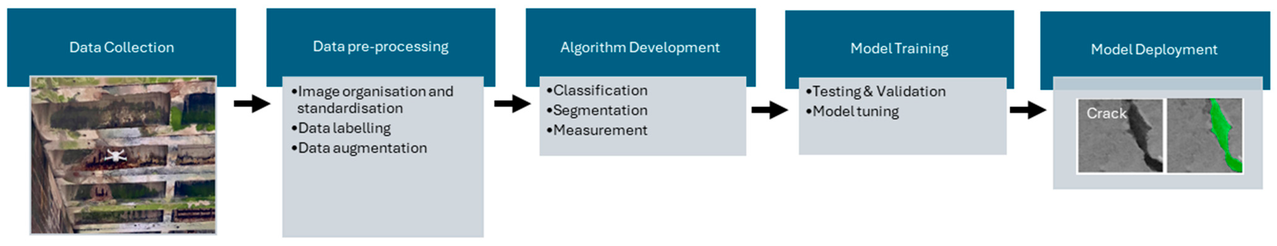
2.1. Overview of Developed Method

The developed method employs DL to detect the presence of concrete cracks in images. Once detected, both crack width and maximum crack width are measured in millimetres. This method was formulated by performing five tasks: data collection, data preprocessing, algorithm development, deep learning training and system deployment. The development process is illustrated in Figure 1—each one of these steps will be further elaborated in subsequent subsections.

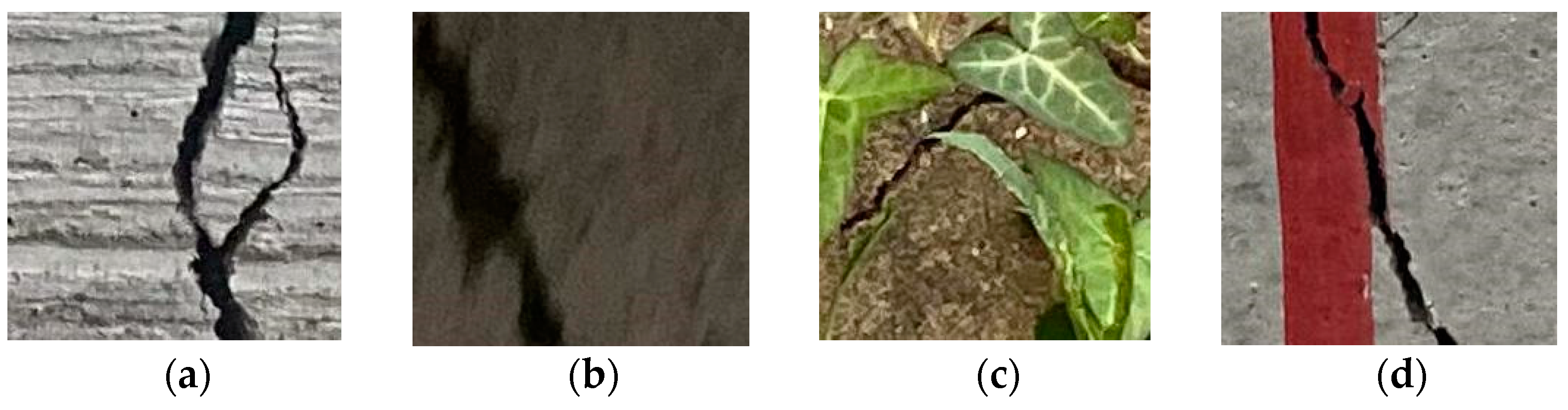
2.2. Data Acquisition

Visual inspections were carried out to acquire visual data, such as videos and images, which was then used to create training, validation and test datasets for the DL models that would be used in the image classification and segmentation tasks. Several image acquisition devices were deployed to various locations to capture a diverse array of visual data.

Table 1. Description of the image acquisition devices used in this study.

Device	Specifications	Data Type	Location Used
DJI Mini 3 pro	- Resolution: 12.1 mega-pixels, f/1.7 - Video frame-rate: 4 K/60 p, 2.7 K/60 p, 1080/120 p	- Images - Videos	- Bridges - Outdoor buildings
iPhone 11 Pro Max	- Resolution: 12 mega-pixels, f/1.8 aperture wide lens (4032 × 3024 pixels)	- Images - Videos	- Bridges - Laboratory - Indoor buildings - Outdoor buildings - Slabs
Nikon D3400 DSLR	- Resolution: 24 mega-pixels (6000 × 4000) - Lens: 18–55 mm Nikon AF-P DX Nikkor	- Images - Videos	- Bridges - Laboratory - Indoor - Outdoor buildings - Slabs

describes these devices, detailing the locations where they were used, and the specific types of data collected. Data was collected from the following locations and specimens:

-

two concrete bridges in South Wales;

-

buildings around the University of South Wales (USW) Treforest Campus;

-

concrete beams, cubes and cylinders from laboratory experiments; and indoor and outdoor concrete slabs.

It was vital to capture a wide range of photos with varying features, as this would ensure that the trained models could perform with significant generalisation capabilities when applied to new, previously unseen data. This was achieved by capturing images of varying quality, in both low and high resolution, and in varied lighting situations. In addition, photos from the dataset with both background noise and foreground occlusions were included. Figure 2 shows the diversity of the images captured.

2.3. Data Pre-Processing

It is important to highlight that, in addition to variability, the quantity of images plays a vital role in the successful training of highly accurate and generalisable crack classification and segmentation models. In the acquisition stage, 297 images (with resolutions of 8000 × 4000, 6000 × 4000 and 4032 × 3024 pixels) were captured. After pre-processing was performed, these full-size images were divided into a total of 5026 images, each measuring 257 × 257 pixels. These images were then used to create a dataset named NYA-Crack-Data.

To increase the size of the dataset, the 5026 images were combined with images from two existing datasets (SDNET2018 [42] and Concrete Crack Images for Classification [43]). The combination of datasets created a new dataset, NYA-Crack-CLS, of 47,026 images that was used to train the classification models.

Table 2. Class distribution of the crack classification dataset.

Dataset	Crack Images	No Crack Images
Our data (NYA-Crack-Data)	2167	2859
SDNET2018	1000	1000
Concrete Crack Images for Classification	20,000	20,000
Total (47,026)	23,167	23,859

shows the class distribution of the combined crack classification dataset.

A similar approach was adopted to create the crack segmentation dataset, NYA-Crack-SEG, with a total of 800 images taken from the following datasets:

• 500 images captured, as described in Section 2.2.
• 150 images from SDNET2018
• 150 images from Concrete Crack Images for Classification

The images in the crack segmentation dataset were labelled by using Roboflow to draw masks around the cracks [44]. The datasets for classification and segmentation were then split into training, validation and testing datasets, at a 70:20:10 ratio, respectively. The next sub-section describes the development of the DL and image processing algorithms for crack classification, segmentation and measurement.

2.4. Algorithm Development

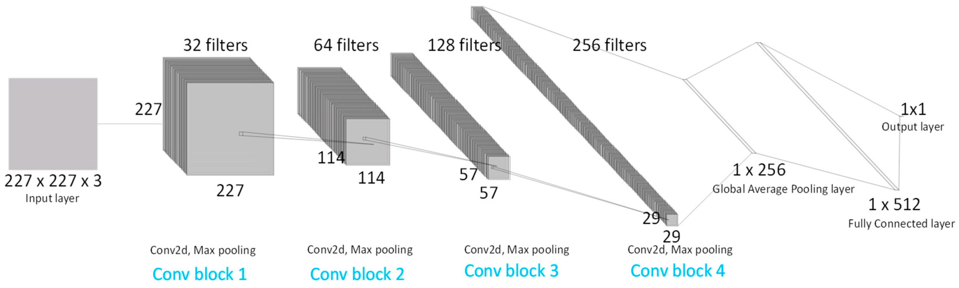
2.4.1. Crack Classification Model

A custom CNN model was developed, using the python programming language [45], for the purpose of classifying collected images from inspections into two categories: cracked or not cracked. Figure 3 depicts the architecture of the model, illustrating the structure, which is comprised of four main blocks of 2D convolutional layers (Conv2D). The first layer in the model is the input layer, which accepts an RGB image of dimensions 227 × 227 × 3; it is followed by the first Conv2D layer, which consists of 32 filters of size 9 × 9 and a ReLu activation function. Padding was used to ensure that the spatial dimensions of the output remained identical to the input, thus preserving the edge information.

The second, third and fourth blocks of layers in the model architecture maintain a similar structure to the first block, with the exception of an increased number of filters that get smaller in each subsequent block: the second, third and fourth Conv2D layers therefore comprise 64 filters of size 7 × 7, 128 filters of size 5 × 5, 256 filters of 3 × 3, respectively. The spatial dimensions of Conv2D’s output are halved every time by the presence of a MaxPooling2D layer of size 2 × 2. The model was trained with the Adaptive Moment Optimisation (ADAM) optimizer, using a learning rate of 0.0001. The optimizer and learning rate were chosen experimentally to find the best results. The output of the model is a binary classification that classifies the input image as either cracked or not cracked. Any image that is classified as cracked is subsequently passed onto the segmentation network for further analysis, with the goal of measuring the crack width along the crack.

2.4.2. Crack Segmentation Model

Two segmentation models were built, a custom U-Net and custom FCN-model. The details of the model architectures are described in this section.

Custom U-Net Model

The custom U-Net model consists of two blocks, an encoder and a decoder block. The first layer of the network before the encoder block is an input layer, which accepts an RGB image of size 160 × 160 × 3. The encoder block has four layers, which each have two convolution layers that can be summarised as follows:

Encoder block:

In layer 1, the first convolution performs convolutions on the input image; it has 64 filters of size 5 × 5, and uses a ReLu activation function. It is followed by a batch normalisation layer. The second convolution layer has the same number of filters as the previous convolution layer, which are also the same size. The convolution layer is followed by a max pooling layer of size 2 × 2, and then by a skip connection layer. The same structure was used for layers 1, 2 and 3, and the only difference between them is the number and size of the filters used in the convolution layers (Layer 2 uses 128 filters of size 3 × 3 while Layer 3 and Layer 4 use 256 and 512 filters of size 3 × 3, respectively).

Middle block:

The middle block connects the encoder and decoder blocks with a convolution layer with 1024 filters of size 3 × 3.

Decoder block:

The decoder block has four layers. The first layer is an upsampling layer that uses a transposed convolution function, and is concatenated with the fourth layer of the encoder block by skip connection. Then two convolution functions with 512 filters of sizes 5 × 5 and 3 × 3 are then applied. The next three layers follow the same format, with a change in the number of filters, with the second, third and fourth layers using 256, 128 and 64 filters respectively. The second, third and fourth layers are concatenated with third, second and first layers of the encoder block, respectively, and us the skip connections. The model was trained using the ADAM optimizer, with a learning rate of 0.0001.

Custom FCN Model

The second custom segmentation model built for crack segmentation was a fully convolutional network (FCN), which used the custom CNN model described in Section 2.4.1 as the backbone for the network. The purpose of the FCN model was to transform an input of an RGB image (size 160 × 160 × 3) to a binary segmentation mask. The custom FCN model was designed to consist of two blocks: The first block (encoder) used the architecture of the custom CNN model and was used for capturing the context of the input image; and the second block, essentially a decoder block, carried out up sampling in four layers. Each layer has a Conv2DTranspose layer for up sampling, and a convolutional layer (Conv2D) that gradually increases the spatial dimension while refining crack features in the image. Layers 1, 2, 3 and 4 make use of 128, 64, 32 and 16 filters, which are all of size 2 × 2. All the layers use a stride of 2 × 2, a ReLu activation function and a padding option (‘same’). The final layer after the decoder block is a convolution layer that concludes with an output of a binary crack mask that has the same spatial dimensions (160 × 160) as the input of the custom CNN model used in the encoding block.

2.4.3. Crack Width Determination

The width of the cracks detected in the images was measured by using image processing techniques proposed in our previous work [5]. However, we made modifications to enhance the method. Instead of using image processing and morphology operations, we used DL-based segmentation to obtain the binary crack masks. These binary crack masks were used as the starting point for the crack measurement process. The crack topology was clearly outlined as a single-pixel-wide skeleton representation by using the medial axis transform method. The distance transform was used to calculate the distance from each pixel in the crack to the medial axis.

The method was used to identify the crack width, which was measured in pixels as the distance from the medial axis to the two outer edges of the crack [5]. The maximum crack width along the length of the segmented crack was identified and highlighted on the image by using a colour bar plot in the image. The pixels along the crack are represented with different colours that represent the size of the crack.

The measured crack width was converted from pixels to millimetres by using the laser calibration method we developed in our previous work [5]. Laser calibration established a relationship between the diameter of the projected laser beam and the distance to the measuring surface. This method was refined, addressing limitations identified in its previous implementation. Enhancements that involved rigorous testing were used to examine the effects of capturing images in scenarios where the laser was not directly perpendicular to the measuring surface, as illustrated in Figure 4.

The experiments resulted in the establishment of a new relationship between the laser diameter and distance to the measuring surface. The new relationship, shown in Equation (1), accounts for the angle of deviation of the laser/camera, relative to the plane perpendicular to the measuring surface.

$${\varnothing }_{\mathrm{r}\mathrm{e}\mathrm{a}\mathrm{l}}=\frac{0.059\mathrm{D}}{\cos \theta }+3.0904 (\mathrm{mm})$$

(1)

where ${\varnothing }_{\mathrm{r}\mathrm{e}\mathrm{a}\mathrm{l}}$ is the actual diameter of the laser in millimetres; $\theta$ is the angle of deviation of the laser/camera, relative to the plane perpendicular to the measuring surface; and D is the distance to the measuring surface.

In most practical cases, images are captured with the camera and laser perpendicular to the measuring surface. Therefore, the angle $\theta$ is assumed to be zero, thus simplifying Equation (1) to Equation (2).

$${\varnothing }_{\mathrm{r}\mathrm{e}\mathrm{a}\mathrm{l}}=0.059\mathrm{D}+3.0904 \left(\mathrm{mm}\right)$$

(2)

Knowing this relationship, a conversion factor, ${\mathsf{\alpha }}_{\mathrm{c}}$, was calculated, as shown in Equation (3)

$${\mathsf{\alpha }}_{\mathrm{c}}=\frac{{\varnothing }_{\mathrm{r}\mathrm{e}\mathrm{a}\mathrm{l}}}{{\varnothing }_{\mathrm{p}\mathrm{x}}} (\mathrm{mm}/\mathrm{pixels})$$

(3)

where ${\mathsf{\alpha }}_{\mathrm{c}}$ is the conversion factor; ${\varnothing }_{\mathrm{r}\mathrm{e}\mathrm{a}\mathrm{l}}$ is the actual diameter of the laser in millimetres; and ${\varnothing }_{\mathrm{p}\mathrm{x}}$ is the diameter of the laser in the image measured in pixels, established by using an algorithm by Nyathi et al. [5]).

The conversion factor enables the accurate conversion of pixels to millimetres by Equation (4), thus allowing crack width to be measured in millimetres.

$${\mathrm{C}}_{\mathrm{w}}\left(\mathrm{m}\mathrm{m}\right)={\mathrm{C}\mathrm{w}}_{\mathrm{p}}\times {\mathsf{\alpha }}_{\mathrm{c}}={\mathrm{C}\mathrm{w}}_{\mathrm{p}}\times \frac{{\varnothing }_{\mathrm{r}\mathrm{e}\mathrm{a}\mathrm{l}}}{{\varnothing }_{\mathrm{p}\mathrm{x}}}$$

(4)

where ${\mathrm{C}}_{\mathrm{w}}$ is the crack width in millimetres; ${\mathrm{C}\mathrm{w}}_{\mathrm{p}}$ is the crack width in pixels; and ${\mathsf{\alpha }}_{\mathrm{c}}$ is the conversion factor in (mm/pixels).

2.5. Performance Evaluation

The performance of the developed model was evaluated by a set of evaluation metrics. For the classification models, accuracy, loss, precision, recall and F1-score were used to assess performance. The segmentation model was evaluated by using the same metrics, but with the addition of the intersection over union (IOU) metric. These metrics are defined below, as follows:

• Accuracy, defined by Equation (5), is the ratio of the correctly classified images to total number of images in the dataset.

  $$\mathrm{A}\mathrm{c}\mathrm{c}\mathrm{u}\mathrm{r}\mathrm{a}\mathrm{c}\mathrm{y}=\frac{\mathrm{T}\mathrm{P}+\mathrm{T}\mathrm{N}}{\mathrm{T}\mathrm{P}+\mathrm{T}\mathrm{N}+\mathrm{F}\mathrm{P}+\mathrm{F}\mathrm{N}}$$

  (5)

  where TP represents True Positives; TN represents True Negatives; FP represents False Positives; and FN represents False Negatives; TP are correctly classified images with cracks; TN are correctly classified images with no cracks; FP are images with no cracks incorrectly classified as having cracks; and FN are images with cracks incorrectly classified as having no cracks.
• Precision, defined by Equation (6), is the ratio of positively classified crack images, true positives, over the total number of classified positives, both true and false.

  $$\mathrm{P}\mathrm{r}\mathrm{e}\mathrm{c}\mathrm{i}\mathrm{s}\mathrm{i}\mathrm{o}\mathrm{n}=\frac{\mathrm{T}\mathrm{P}}{\mathrm{T}\mathrm{P}+\mathrm{F}\mathrm{P}}$$

  (6)
• Recall, also referred to as sensitivity, is defined by Equation (7); it is the ratio of correctly classified cracks over the total number of crack observations.

  $$\mathrm{R}\mathrm{e}\mathrm{c}\mathrm{a}\mathrm{l}\mathrm{l}=\frac{\mathrm{T}\mathrm{P}}{\mathrm{T}\mathrm{P}+\mathrm{F}\mathrm{N}}$$

  (7)
• F1 score is used to calculate the weighted average of Precision and Recall and is defined by Equation (8). F1 scores range from 0 to 1, with values closer to one indicating a good balance between precision and recall.

  $$\text{F1 score}=\frac{2\mathrm{T}\mathrm{P}}{2\mathrm{T}\mathrm{P}+\mathrm{F}\mathrm{P}+\mathrm{F}\mathrm{N}}$$

  (8)
• IOU, defined in Equation (9), is the measure of how much the predicted crack segmentation area overlaps (intersects) with the actual crack area, relative to the total area of predicted crack segmentation and actual crack.

  $$\mathrm{I}\mathrm{O}\mathrm{U}=\frac{\mathrm{A}\mathrm{r}\mathrm{e}\mathrm{a} \mathrm{o}\mathrm{f} \mathrm{I}\mathrm{n}\mathrm{t}\mathrm{e}\mathrm{r}\mathrm{s}\mathrm{e}\mathrm{c}\mathrm{t}\mathrm{i}\mathrm{o}\mathrm{n}}{\mathrm{A}\mathrm{r}\mathrm{e}\mathrm{a} \mathrm{o}\mathrm{f} \mathrm{U}\mathrm{n}\mathrm{i}\mathrm{o}\mathrm{n}}$$

  (9)

2.6. Implementation

To carry out crack classification, segmentation and measurement by using the methods described above, the following steps must be taken:

• Capture images or videos using the image acquisition device of choice.
• If videos were captured, pre-process them by converting the videos into image frames.
• Feed the collected images into the classification model, which will classify the images as ‘cracked’ or ‘uncracked’, and save in the relevant folder.
• Segment the images in the ‘cracked’ folder by passing them as an input to the segmentation model; this segments the images, producing a binary mask of the crack.
• Apply the measurement algorithm to binary masks to obtain a visual output, showing the crack width and location of maximum crack width.
• To convert the crack width from pixels to millimetres, detect the laser in the image and measure its pixel diameter. Use Equations (3) and (4) to convert the pixels to millimetres.

The next section presents and discusses the results obtained from the implementation of the developed method.

3. Results and Discussion

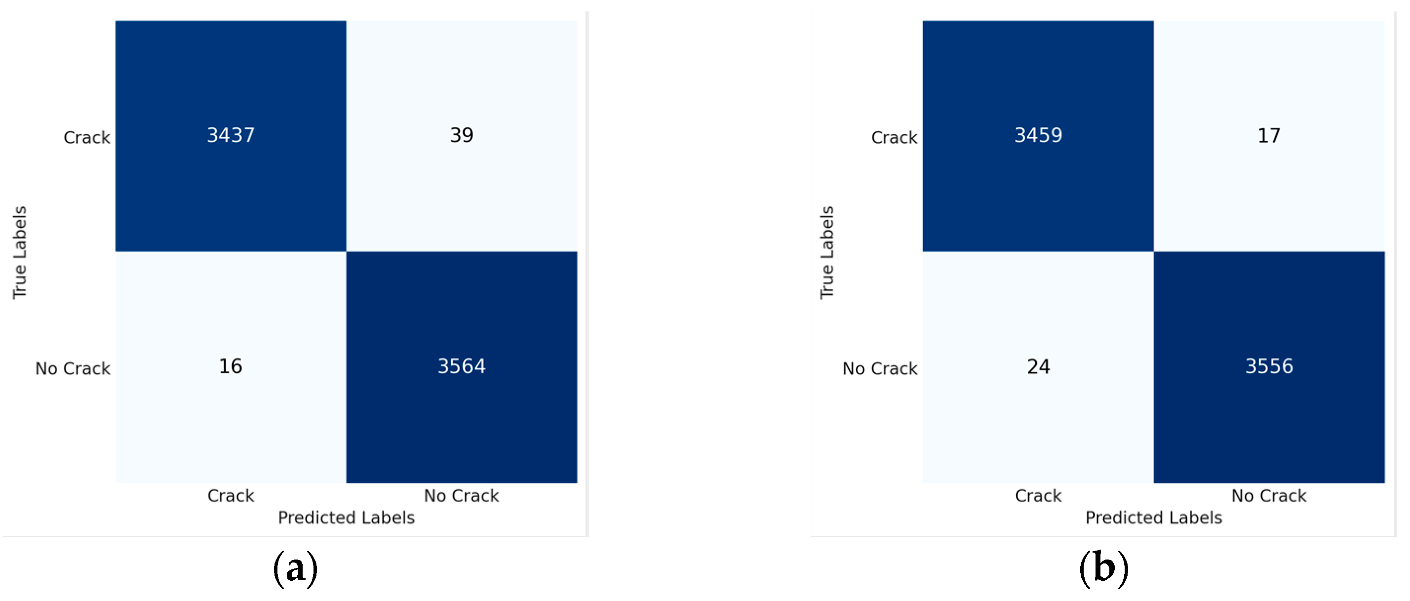
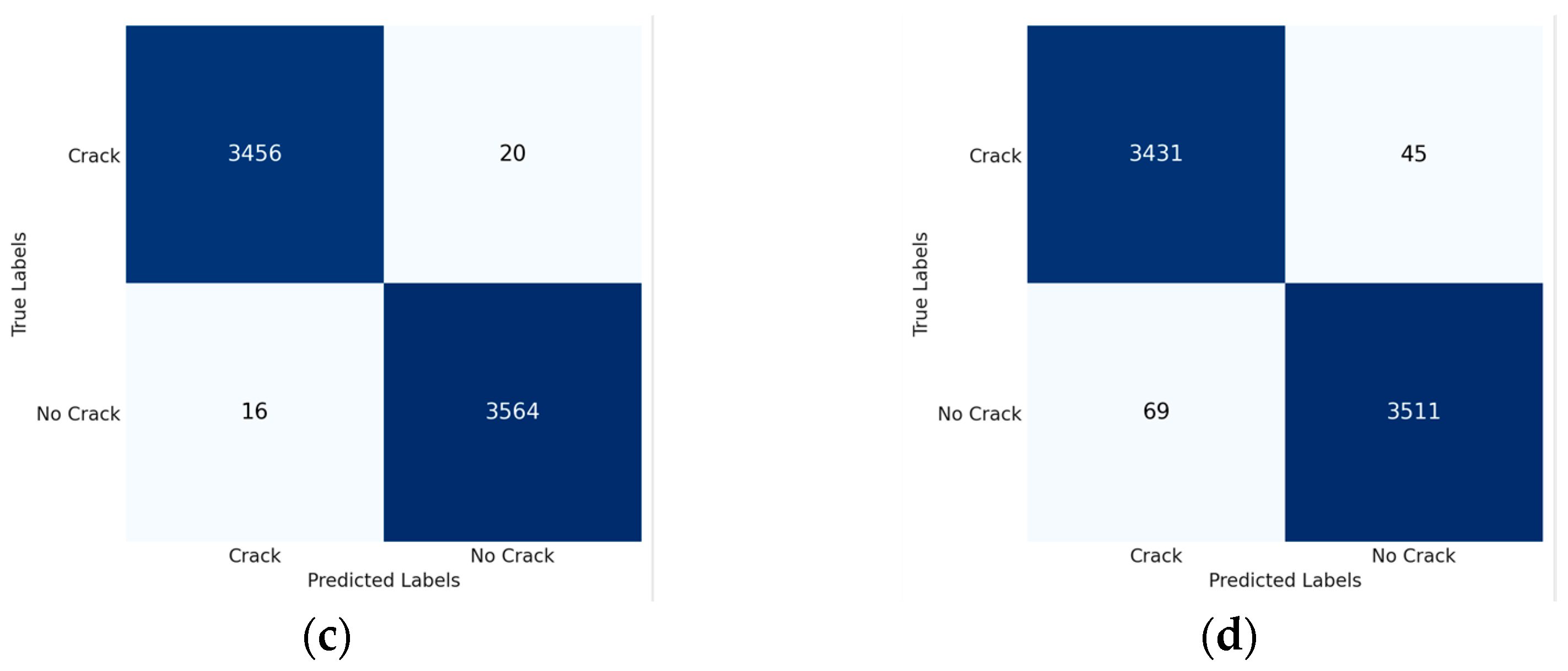
This section evaluates the developed methods of crack detection and crack measurement. The performance of the crack classification model is evaluated on the test dataset generated from the combination of our dataset with the two open-source datasets (SDNET2018 [42] and Concrete Crack Images for Classification [43]). The performance of the developed crack width measurement method was evaluated by comparing the measurements to manual measurements.

3.1. Classification

The performance of the custom model was compared against widely used pre-trained CNN models for a variety of classification tasks, including concrete crack classification. The models used for comparison were Inception V4, VGG16 and DenseNet121. Figure 4 shows the confusion matrices of the custom CNN model and the four pre-trained CNN models used to judge the performance of the custom CNN. As shown in Figure 4a, class 0 and class 1 represent Crack and No Crack, respectively. The diagonal blocks in the confusion matrices represent the number of correctly classified classes in the test dataset, and the off-diagonal blocks represent misclassified classes. It can be seen from Figure 5 that the best performing models (in terms of classification of the No Crack class) are Custom CNN and VGG16, which performed at par, classifying 3564 images correctly. The custom CNN model misclassified 39 images of cracks as having no cracks, and was outperformed by VGG16 and Inception V4, which misclassified 20 and 17 images, respectively.

Furthermore, the performance of the models was validated by using the testing accuracy, loss, precision, recall and F1-score metrics. The results presented in

Table 3. Performance evaluation of concrete crack classification on unseen image data.

Model	Testing		Precision	Recall	F1-Score	Training Time (min)
	Accuracy	Loss
Custom CNN	99.22	0.0340	0.9954	0.9888	0.9921	35.9
Inception V4	99.87	0.0049	0.9931	0.9951	0.9941	66.5
VGG16	99.89	0.0041	0.9954	0.9943	0.9949	46.2
DenseNet121	98.21	0.0543	0.9803	0.9870	0.9836	60.5

show that while the custom CNN did not obtain the highest testing accuracy, it did achieve a notably high accuracy of 99.22%. The precision metric was also used to assess the performance of the models. The custom CNN model was once again tied to the VGG16 model, with both achieving the highest precision of 0.9954. The recall, accuracy and F1-score for all models were all high (above 0.98). The performance of the custom CNN architecture may be improved by further training on a larger and more varied dataset. Further hyperparameter tuning, combined with an increase in training epochs, could also lead to improved results. Custom CNN was chosen over other models because of its model simplicity, which subsequently results in lower computational cost, when compared to the other pre-trained models. This is evidenced in

Table 4. Comparison of number parameters for each of the classification models.

Model	Total Parameters	Trainable Parameters	Non-Trainable Parameters
Custom CNN	409,442	409,314	128
Inception V4	55,912,674	55,852,130	60,544
VGG16	15,242,050	15,242,050	0
DenseNet121	8,089,154	8,005,506	83,648

, which shows that the custom CNN model has a smaller number of parameters than the other models. Due to its simplicity, the custom CNN had the shortest training time of only 35.9 min and this, combined with its high accuracy and precision, make it an attractive choice for general inspections that seek to determine the presence of cracks, and sort images accordingly for further analysis, if needed.

Passing the collected images through the classification model before carrying out crack segmentation offers several benefits:

• improved efficiency by filtering out irrelevant images without cracks, ensuring the DL segmentation model only processes images with cracks;
• reduction in computational cost, due to only images with cracks being segmented;
• improved accuracy of the segmentation model, because only images known to have cracks are segmented, minimising the likelihood of false positive segmentations;
• lastly, the classification model is designed to save output in cracked or uncracked folders, thereby continuously expanding the dataset size.

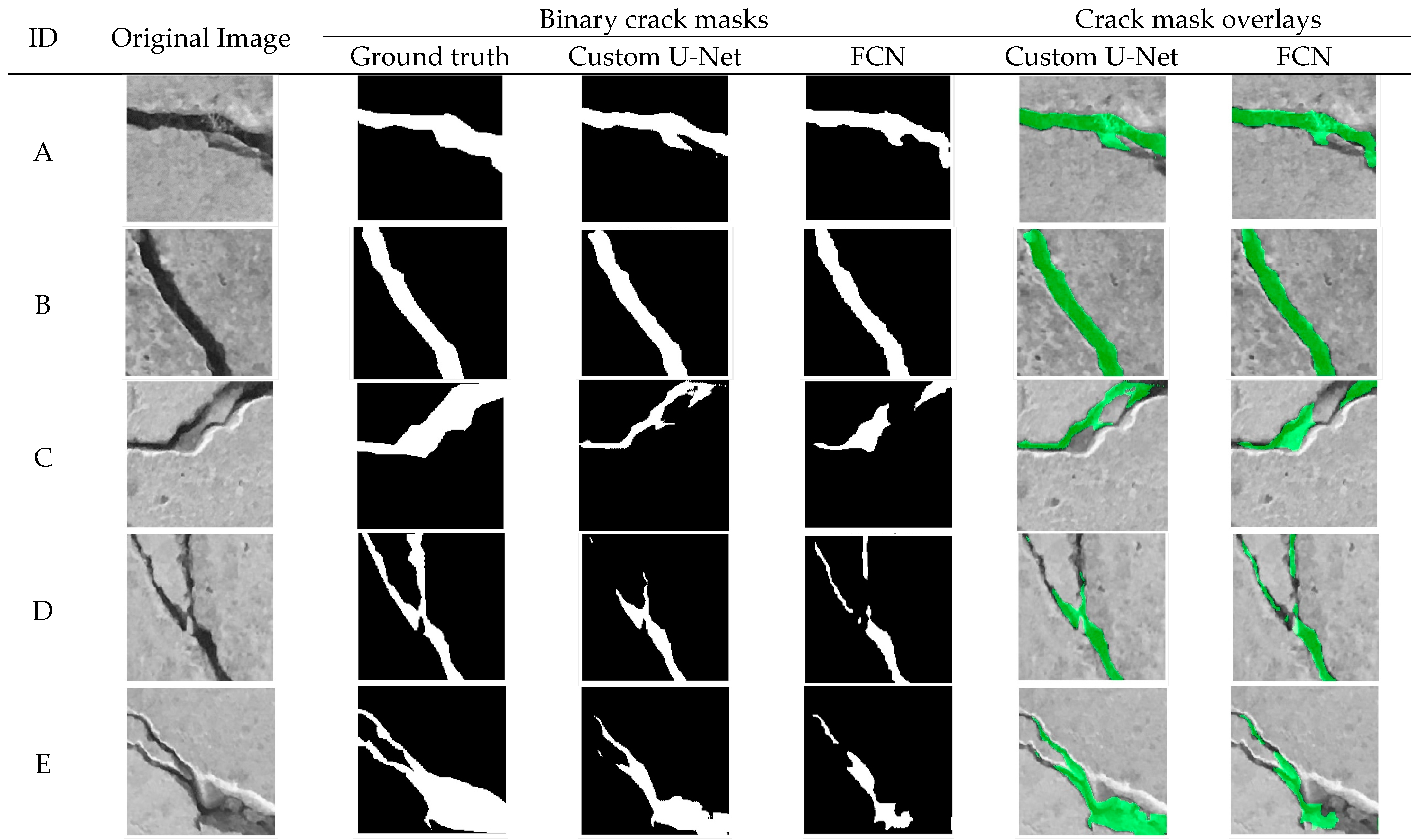
3.2. Segmentation

A test dataset of images not previously seen by the two segmentation models was used to evaluate the custom U-Net and FCN models, and a visual representation of the performance of the models is presented in Figure 6. The binary crack masks and overlain masks obtained using the custom U-Net and FCN models were compared to ground truth segmentations. It can be seen from Figure 6 that the custom U-Net model, when compared to the custom FCN model, created segmentation masks closer to ground truth. The custom U-Net crack masks were, apart from crack D, observed to be more continuous, in comparison to the custom FCN masks. The performance of the models was further validated by the evaluation metrics shown in

Table 5. Performance evaluation results of the segmentation models.

Model	Accuracy	IoU	Precision	Recall	F1-Score
Custom U-Net	96.54	0.6295	0.7174	0.8371	0.7726
Custom FCN	95.88	0.5900	0.6897	0.8031	0.7421

, which confirms the custom U-Net model achieved a higher testing accuracy of 96.54% when compared to the custom FCN model, which achieved 95.88%; the custom U-net model also achieved better performance in IoU, precision, recall and F1-scores, with values of 0.6295, 0.7174, 0.8371 and 0.7726, respectively.

The custom U-Net model was chosen as the segmentation model. The next subsection details how the binary crack masks, which were obtained using the custom U-Net model, were utilised for concrete crack width measurement.

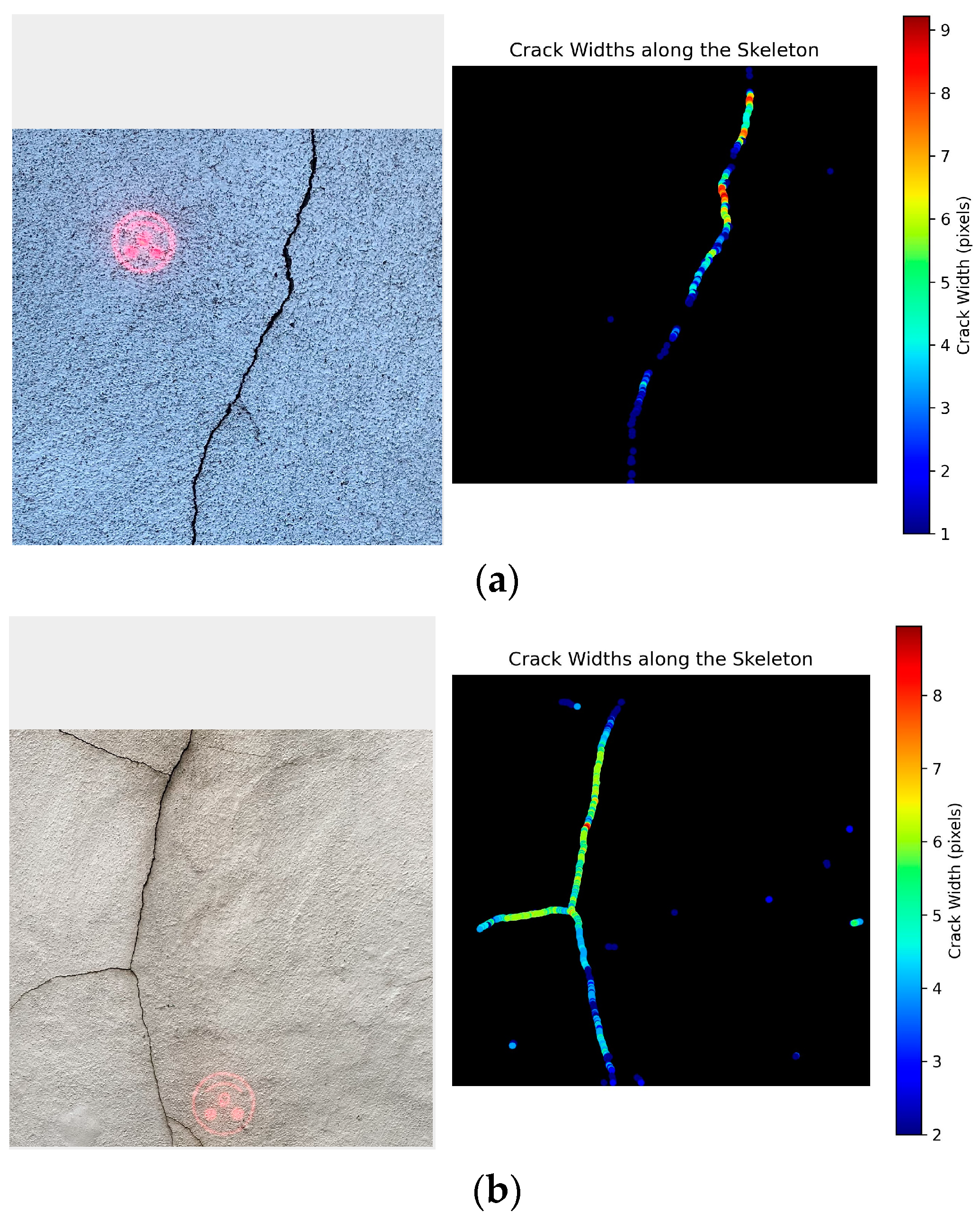
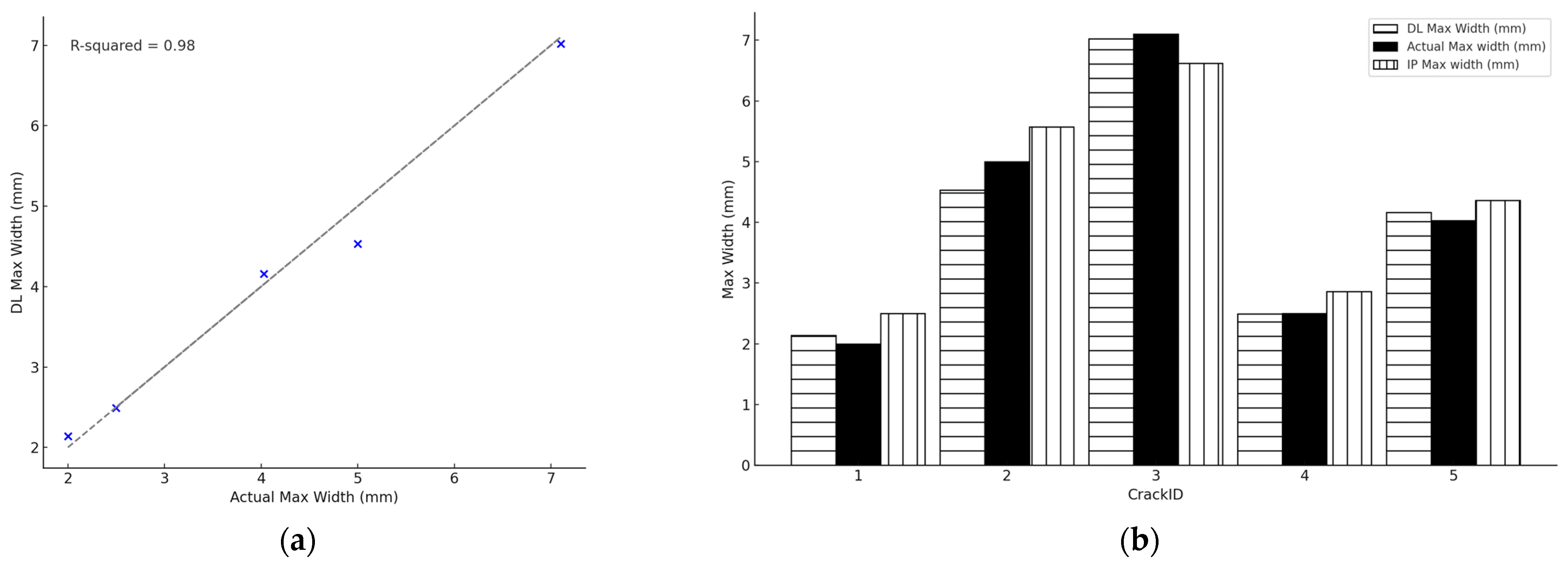
3.3. Crack Width Calculations

The performance of the developed method of crack width measurement was validated by testing it on a set of six images, which were captured under different conditions, such as indoors, outdoors and with a high- and low-resolution camera. The actual crack widths of the cracks were measured by using a vernier caliper. The images of cracks were segmented by using the custom U-Net model to create binary crack masks. The binary crack mask applied the medial axis transform algorithm to measure the crack width in pixels. The enhanced laser calibration technique was used to convert the pixel crack widths to millimetres by multiplying the pixel crack width by the conversion factor. Figure 7 illustrates the process by showing two cracks, and presenting the original image alongside a binary mask, which visually represents the measured crack widths in pixels by using a colour bar scale. Figure 7 also shows that the proposed crack width successfully identifies the section in the crack with the maximum crack width, and also demonstrates the model’s ability to perform well with variable data: here it can be observed that the crack images differ in texture when compared to the Figure 6 images.

The maximum cracks widths of all the measured cracks are presented in

Table 6. Crack width measurement results, using DL segmented crack masks.

Crack ID	Conversion Factor	Measured Max Width (Pixels)	Converted Max Width (mm)	Actual Max Width (mm)	Absolute Error (mm)
1	0.357	6.00	2.14	2.00	0.14
2	0.507	8.94	4.53	5.00	0.47
3	0.351	20.0	7.02	7.10	0.08
4	0.275	9.06	2.49	2.50	0.01
5	0.205	20.3	4.16	4.03	0.13

, which shows that the method measured maximum crack width with a high accuracy. Crack 4 was the most accurately measured crack, with an actual maximum crack width of 2.5 mm, and a proposed method measurement of 2.49 mm: this absolute error of 0.01 mm was the smallest absolute error observed in this experiment. The largest absolute error (of 0.47 mm) was observed in Crack 2, where the actual maximum crack width was 5.00 mm, but measured to be 4.53 mm. The mean absolute error (MAE) of the method was calculated to be 0.16 mm.

The accuracy of the proposed method depends on the quality of the crack masks generated by the U-Net segmentation model. Figure 6 showed that, when it comes to completely masking the entire crack region, the performance of the custom U-Net model still has room for improvement. Better masks can be achieved by training the model with more images, adjusting training parameters and enhancing the model architecture. We anticipate that these enhancements will lead to the improved accuracy of the crack width measurement method.

The overall performance of the method using DL segmentation is visualised in Figure 8. Figure 8a shows a comparison between the maximum crack widths measured with the DL method versus the actual maximum crack widths. The dashed line represents points where the measured values are equal to the actual values. It can be seen that the maximum crack width values were close to the actual values, and this is supported by a high R-squared value of 0.98.

The performance of the developed measurement method was further evaluated by a comparison of three cases:

(1)

DL Max width: Maximum crack width measured from crack images segmented by using DL;

(2)

IP Max width: Maximum crack width measured from crack images segmented by using image processing (IP) algorithms;

(3)

Actual Max width: Maximum crack widths measured manually on site.

In Figure 8b, the maximum crack widths measured with DL and IP methods are compared to the actual crack widths. As expected, the DL method outperformed the IP method, with maximum crack width measurement values closer to the actual maximum crack width. In all cases, the maximum crack widths measured with the IP method had, when compared to the DL method, larger errors, relative to the actual maximum crack widths.

4. Conclusions

This paper presented an enhanced, novel method for detecting and measuring concrete crack width in millimetres by using deep learning and a laser calibration technique. The classification, segmentation and measurement tasks were performed with high accuracy. However, one major limitation of the method is the training dataset size, especially for the segmentation model. A larger dataset and hyperparameter tuning of the model will significantly improve accuracy.

In closing, the following conclusions can be drawn from this study:

• A computationally effective approach that reduces false positives, which carries out crack segmentation by first passing images through a classification model has been proposed.
• DL segmentation yielded better results when compared to conventional image processing algorithms. In addition, DL offers better generalisation and quicker segmentation, and does not need an expert to carry out manual parameter selection.
• An enhanced laser calibration technique has been developed and applied successfully, meaning concrete crack width can be measured in millimetres.
• The use of the laser eliminates the need for physical markers to be attached to the surface being measured. This promotes safer inspections, which can be achieved by simply deploying a drone with the laser system, especially in hard-to-reach areas.

References

1. Choudhary, G.K.; Dey, S. Crack Detection in Concrete Surfaces Using Image Processing, Fuzzy Logic, and Neural Networks. In Proceedings of the 2012 IEEE 5th International Conference on Advanced Computational Intelligence, ICACI 2012, Nanjing, China, 18–20 October 2012; pp. 404–411. [Google Scholar] [CrossRef]
2. Park, S.E.; Eem, S.H.; Jeon, H. Concrete Crack Detection and Quantification Using Deep Learning and Structured Light. Constr. Build. Mater. 2020, 252, 119096. [Google Scholar] [CrossRef]
3. Frangopol, D.M.; Curley, J.P. Effects of Damage and Redundancy on Structural Reliability. J. Struct. Eng. 1987, 113, 1533–1549. [Google Scholar] [CrossRef]
4. Avci, O.; Abdeljaber, O.; Kiranyaz, S.; Hussein, M.; Gabbouj, M.; Inman, D.J. A Review of Vibration-Based Damage Detection in Civil Structures: From Traditional Methods to Machine Learning and Deep Learning Applications. Mech. Syst. Signal Process. 2021, 147, 107077. [Google Scholar] [CrossRef]
5. Nyathi, M.A.; Bai, J.; Wilson, I.D. Concrete Crack Width Measurement Using a Laser Beam and Image Processing Algorithms. Appl. Sci. 2023, 13, 4981. [Google Scholar] [CrossRef]
6. Thagunna, G. Building Cracks—Causes and Remedies. Int. J. Adv. Struct. Geotech. Eng. 2015, 4, 16–20. [Google Scholar]
7. Munawar, H.S.; Hammad, A.W.A.; Haddad, A.; Soares, C.A.P.; Waller, S.T. Image-Based Crack Detection Methods: A Review. Infrastructures 2021, 6, 115. [Google Scholar] [CrossRef]
8. Golding, V.P.; Gharineiat, Z.; Munawar, H.S.; Ullah, F. Crack Detection in Concrete Structures Using Deep Learning. Sustainability 2022, 14, 8117. [Google Scholar] [CrossRef]
9. Ai, D.; Jiang, G.; Lam, S.K.; He, P.; Li, C. Computer Vision Framework for Crack Detection of Civil Infrastructure—A Review. Eng. Appl. Artif. Intell. 2023, 117, 105478. [Google Scholar] [CrossRef]
10. Fujita, Y.; Hamamoto, Y. A Robust Automatic Crack Detection Method from Noisy Concrete Surfaces. Mach. Vis. Appl. 2010, 22, 245–254. [Google Scholar] [CrossRef]
11. Hoang, N.D. Detection of Surface Crack in Building Structures Using Image Processing Technique with an Improved Otsu Method for Image Thresholding. Adv. Civ. Eng. 2018, 2018, 3924120. [Google Scholar] [CrossRef]
12. Canny, J. A Computational Approach to Edge Detection. IEEE Trans. Pattern Anal. Mach. Intell. 1986, PAMI-8, 679–698. [Google Scholar] [CrossRef]
13. Zhao, H.; Qin, G.; Wang, X. Improvement of Canny Algorithm Based on Pavement Edge Detection. In Proceedings of the 2010 3rd International Congress on Image and Signal Processing, CISP 2010, Yantai, China, 16–18 October 2010; Volume 2, pp. 964–967. [Google Scholar] [CrossRef]
14. Ioli, F.; Pinto, A.; Pinto, L. Uav Photogrammetry for Metric Evaluation of Concrete Bridge Cracks. Int. Arch. Photogramm. Remote Sens. Spat. Inf. Sci. 2022, XLIII-B2-2, 1025–1032. [Google Scholar] [CrossRef]
15. Kim, H.; Ahn, E.; Cho, S.; Shin, M.; Sim, S.H. Comparative Analysis of Image Binarization Methods for Crack Identification in Concrete Structures. Cem. Concr. Res. 2017, 99, 53–61. [Google Scholar] [CrossRef]
16. Kim, H.; Lee, J.; Ahn, E.; Cho, S.; Shin, M.; Sim, S.H. Concrete Crack Identification Using a UAV Incorporating Hybrid Image Processing. Sensors 2017, 17, 2052. [Google Scholar] [CrossRef] [PubMed]
17. Yang, X.; Li, H.; Yu, Y.; Luo, X.; Huang, T.; Yang, X. Automatic Pixel-Level Crack Detection and Measurement Using Fully Convolutional Network. Comput.-Aided Civ. Infrastruct. Eng. 2018, 33, 1090–1109. [Google Scholar] [CrossRef]
18. Silva, W.R.L.d.; Lucena, D.S.d. Concrete Cracks Detection Based on Deep Learning Image Classification. Proceedings 2018, 2, 489. [Google Scholar] [CrossRef]
19. Kim, H.; Ahn, E.; Shin, M.; Sim, S.H. Crack and Noncrack Classification from Concrete Surface Images Using Machine Learning. Struct. Health Monit. 2018, 18, 725–738. [Google Scholar] [CrossRef]
20. Liu, Y.; Yeoh, J.K.W. Automated Crack Pattern Recognition from Images for Condition Assessment of Concrete Structures. Autom. Constr. 2021, 128, 103765. [Google Scholar] [CrossRef]
21. Uwanuakwa, I.D.; Idoko, J.B.; Mbadike, E.; Reşatoǧlu, R.; Alaneme, G. Application of Deep Learning in Structural Health Management of Concrete Structures. Proc. Inst. Civ. Eng.—Bridge Eng. 2022, 1–8. [Google Scholar] [CrossRef]
22. Gao, Y.; Mosalam, K.M. Deep Transfer Learning for Image-Based Structural Damage Recognition. Comput.-Aided Civ. Infrastruct. Eng. 2018, 33, 748–768. [Google Scholar] [CrossRef]
23. Ronneberger, O.; Fischer, P.; Brox, T. U-Net: Convolutional Networks for Biomedical Image Segmentation. In Proceedings of the 18th International Conference on Medical Image Computing and Computer-Assisted Intervention, Munich, Germany, 5–9 October 2015; Volume 9351, pp. 234–241. [Google Scholar] [CrossRef]
24. Liu, Z.; Cao, Y.; Wang, Y.; Wang, W. Computer Vision-Based Concrete Crack Detection Using U-Net Fully Convolutional Networks. Autom. Constr. 2019, 104, 129–139. [Google Scholar] [CrossRef]
25. Zhao, S.; Kang, F.; Li, J. Non-Contact Crack Visual Measurement System Combining Improved U-Net Algorithm and Canny Edge Detection Method with Laser Rangefinder and Camera. Appl. Sci. 2022, 12, 10651. [Google Scholar] [CrossRef]
26. Mirzazade, A.; Popescu, C.; Gonzalez-Libreros, J.; Blanksvärd, T.; Täljsten, B.; Sas, G. Semi-Autonomous Inspection for Concrete Structures Using Digital Models and a Hybrid Approach Based on Deep Learning and Photogrammetry. J. Civ. Struct. Health Monit. 2023, 13, 1633–1652. [Google Scholar] [CrossRef]
27. Zhao, W.; Liu, Y.; Zhang, J.; Shao, Y.; Shu, J. Automatic Pixel-Level Crack Detection and Evaluation of Concrete Structures Using Deep Learning. Struct. Control Health Monit. 2022, 29, e2981. [Google Scholar] [CrossRef]
28. Chaiyasarn, K.; Buatik, A.; Mohamad, H.; Zhou, M.; Kongsilp, S.; Poovarodom, N. Integrated Pixel-Level CNN-FCN Crack Detection via Photogrammetric 3D Texture Mapping of Concrete Structures. Autom. Constr. 2022, 140, 104388. [Google Scholar] [CrossRef]
29. Dung, C.V.; Anh, L.D. Autonomous Concrete Crack Detection Using Deep Fully Convolutional Neural Network. Autom. Constr. 2019, 99, 52–58. [Google Scholar] [CrossRef]
30. Ye, X.W.; Jin, T.; Chen, P.Y. Structural Crack Detection Using Deep Learning–Based Fully Convolutional Networks. Adv. Struct. Eng. 2019, 22, 3412–3419. [Google Scholar] [CrossRef]
31. Ren, Y.; Huang, J.; Hong, Z.; Lu, W.; Yin, J.; Zou, L.; Shen, X. Image-Based Concrete Crack Detection in Tunnels Using Deep Fully Convolutional Networks. Constr. Build. Mater. 2020, 234, 117367. [Google Scholar] [CrossRef]
32. Kang, D.; Benipal, S.S.; Gopal, D.L.; Cha, Y.J. Hybrid Pixel-Level Concrete Crack Segmentation and Quantification across Complex Backgrounds Using Deep Learning. Autom. Constr. 2020, 118, 103291. [Google Scholar] [CrossRef]
33. Yu, Z.; Shen, Y.; Sun, Z.; Chen, J.; Gang, W. Cracklab: A High-Precision and Efficient Concrete Crack Segmentation and Quantification Network. Dev. Built Environ. 2022, 12, 100088. [Google Scholar] [CrossRef]
34. Chen, L.C.; Zhu, Y.; Papandreou, G.; Schroff, F.; Adam, H. Encoder-Decoder with Atrous Separable Convolution for Semantic Image Segmentation. In Proceedings of the European Conference on Computer Vision 2018, Munich, Germany, 8–14 September 2018; Volume 11211, pp. 833–851. [Google Scholar] [CrossRef]
35. Mishra, M.; Jain, V.; Saurabh, S.K.; Singh, K.; Damodar, M. Two-Stage Method Based on the You Only Look Once Framework and Image Segmentation for Crack Detection in Concrete Structures. Archit. Struct. Constr. 2022, 1, 429–446. [Google Scholar] [CrossRef]
36. Tomczak, K.; Jakubowski, J.; Fiołek, P. Method for Assessment of Changes in the Width of Cracks in Cement Composites with Use of Computer Image Processing and Analysis. Stud. Geotech. Mech. 2017, 39, 73–80. [Google Scholar] [CrossRef]
37. Ito, A.; Aoki, Y.; Hashimoto, S. Accurate Extraction and Measurement of Fine Cracks from Concrete Block Surface Image. In Proceedings of the IEEE 2002 28th Annual Conference of the Industrial Electronics Society, IECON 02, Seville, Spain, 5–8 November 2002; Volume 3, pp. 2202–2207. [Google Scholar] [CrossRef]
38. Peng, X.; Zhong, X.; Zhao, C.; Chen, A.; Zhang, T. A UAV-Based Machine Vision Method for Bridge Crack Recognition and Width Quantification through Hybrid Feature Learning. Constr. Build. Mater. 2021, 299, 123896. [Google Scholar] [CrossRef]
39. Li, S.; Zhao, X. Automatic Crack Detection and Measurement of Concrete Structure Using Convolutional Encoder-Decoder Network. IEEE Access 2020, 8, 134602–134618. [Google Scholar] [CrossRef]
40. Kim, B.; Cho, S. Image-Based Concrete Crack Assessment Using Mask and Region-Based Convolutional Neural Network. Struct. Control Health Monit. 2019, 26, e2381. [Google Scholar] [CrossRef]
41. Jeong, H.; Jeong, B.; Han, M.; Cho, D. Analysis of Fine Crack Images Using Image Processing Technique and High-Resolution Camera. Appl. Sci. 2021, 11, 9714. [Google Scholar] [CrossRef]
42. Dorafshan, S.; Thomas, R.J.; Maguire, M. SDNET2018: An Annotated Image Dataset for Non-Contact Concrete Crack Detection Using Deep Convolutional Neural Networks. Data Brief 2018, 21, 1664–1668. [Google Scholar] [CrossRef] [PubMed]
43. Özgenel, Ç.F.; Gönenç Sorguç, A. Performance Comparison of Pretrained Convolutional Neural Networks on Crack Detection in Buildings. In Proceedings of the 35th International Symposium on Automation and Robotics in Construction, Berlin, Germany, 20–25 July 2018; Volume 35, pp. 1–8. [Google Scholar]
44. Roboflow Inc. Roboflow Annotate: Label Faster Than Ever. Available online: https://roboflow.com/annotate (accessed on 3 September 2023).
45. Python Software Foundation the Python Language Reference. Available online: https://docs.python.org/3/reference/index.html (accessed on 1 August 2023).
Figure 1. Overview of the methodology used to develop the crack detection and measurement system.
Metrology 04 00005 g001
Figure 2. Different types of images included in the concrete crack dataset (a) high resolution (b) low resolution/blurry (c) foreground occlusions (d) graffiti markings.
Metrology 04 00005 g002
Figure 3. Architecture of custom CNN model.
Metrology 04 00005 g003
Figure 4. The effect of varying the distance from the measuring surface and the angle of laser beam projection.
Metrology 04 00005 g004
Figure 5. Confusion matrices obtained from the CNN models using the test dataset (a) Custom CNN, (b) Inception V4, (c) VGG16 and (d) DenseNet121.
Metrology 04 00005 g005aMetrology 04 00005 g005b
Figure 6. Comparison of original concrete crack images and ground truth masks with crack masks generated with the two deep learning models.
Metrology 04 00005 g006
Figure 7. Measured crack widths displayed on segmented crack masks and generated using the custom U-Net model for (a) Crack 1 and (b) Crack 2.
Metrology 04 00005 g007
Figure 8. (a) Performance of the DL measured crack widths, compared to the actual maximum crack width values. (b) A comparison of the DL, IP measured maximum crack widths and the actual maximum crack widths.
Metrology 04 00005 g008