Article

Experimental Investigation on the Transfer Behavior and Environmental Influences of Low-Noise Integrated Electronic Piezoelectric Acceleration Sensors

1
Institute of Concrete Structures, TUD Dresden University of Technology, 01062 Dresden, Germany
2
Division 7.2 Buildings and Structures, Federal Institute of Materials Research and Testing (BAM), 12205 Berlin, Germany
*
Author to whom correspondence should be addressed.
Metrology 2024, 4(1), 46-65; https://doi.org/10.3390/metrology4010004
Submission received: 18 December 2023 / Revised: 11 January 2024 / Accepted: 22 January 2024 / Published: 1 February 2024

Abstract

:
Acceleration sensors are vital for assessing engineering structures by measuring properties like natural frequencies. In practice, engineering structures often have low natural frequencies and face harsh environmental conditions. Understanding sensor behavior on such structures is crucial for reliable measurements. The research focus is on understanding the behavior of acceleration sensors in harsh environmental conditions within the low-frequency acceleration range. The main question is how to distinguish sensor behavior from structural influences to minimize errors in assessing engineering structure conditions. To investigate this, the sensors are tested using a long-stroke calibration unit under varying temperature and humidity conditions. Additionally, a mini-monitoring system configured with four IEPE sensors is applied to a small-scale support structure within a climate chamber. For the evaluation, a signal-energy approach is employed to distinguish sensor behavior from structural behavior. The findings show that IEPE sensors display temperature-dependent nonlinear transmission behavior within the low-frequency acceleration range, with humidity having negligible impact. To ensure accurate engineering structure assessment, it is crucial to separate sensor behavior from structural influences using signal energy in the time domain. This study underscores the need to compensate for systematic effects, preventing the underestimation of vibration energy at low temperatures and overestimation at higher temperatures when using IEPE sensors for engineering structure monitoring.

1. Introduction

Structural Health Monitoring (SHM) and Non-Destructive Evaluation (NDE) have become increasingly used in practice to enhance periodic inspections of engineering structures with continuous measurement data [1,2,3,4,5]. Accelerometers can be used to determine the dynamic properties of these structures (e.g., eigenfrequencies, modal eigenmodes, and operating mode shapes) to detect structural damage [6,7,8,9,10]. Hence, these sensors are often used for the monitoring of engineering structures such as bridges or wind turbine towers. These structures typically have low eigenfrequencies due to their geometry, in particular their high modal mass combined with low modal stiffness. Commonly, the first modal eigenfrequency of road bridges ranges from 2 Hz to 5 Hz and that of wind turbine towers is between 0.2 Hz and 1.0 Hz [11,12,13]. Such low eigenfrequencies cannot be reliably measured easily. This is often a problem in practice because these boundary conditions do not align with the standard use case for accelerometers [7,14,15,16]. DC-coupled MEMS (Micro-Electro-Mechanical System) sensors have often been used in the low-frequency range due to their linear response in this range and their capability to measure constant accelerations, such as gravity [17]. For example, in [18], Zanelli et al. developed a monitoring system for bridge mode identification using wireless MEMS sensors as an alternative to wired MEMS sensors. To evaluate the sensor performance, some prototypes were installed on a railway bridge for a field test and data were collected showing the low-frequency system behavior of the bridge. Bedon et al. developed an MEMS sensor prototype in [19], which was calibrated employing laboratory tests. The experimental validation of the MEMS accelerometers was carried out using the example of the cable-stayed bridge in Pietratagliata (Italy), which has natural frequencies of approx. 2 Hz.
However, these MEMS sensors have a low signal-to-noise ratio (SNR). Alternatively, lower-noise Integrated Electronic Piezoelectric (IEPE) accelerometers are also employed, even though they are larger in size and generally come with a higher unit cost. IEPE sensors have a frequency-dependent response and operate on an AC-coupled signal conditioner. To achieve precise measurements at the limits of the IEPE sensor, exact knowledge of its behavior is essential. Consequently, frequency-dependent calibration of the IEPE sensors is imperative. There are various methods for calibrating accelerometers following ISO 16063 [20] in conjunction with DIN EN ISO/IEC 17025 [21], including gravity-based calibration, shock calibration by comparison with a reference transducer, and the calibration of vibration calibrators for use on site. The calibration method used in this paper is described in DIN ISO 16063-21 [20,22]. This method utilizes a long-stroke shaker to generate a substantial displacement, ensuring a sufficiently large measurement signal amplitude. Within the low-frequency vibration range, the sensitivity and phase shift of the sensor to be calibrated are determined with the aid of a reference transducer. In addition to long stroke distances, there are alternative calibration methods. For example, Olivares et al. in [23] and Jonscher et al. in [24] utilized an inclined centrifuge to calibrate acceleration sensors, relying on the earth’s gravitational field and the centrifuge’s inclination rather than stroke distance.
To use IEPE sensors in practice reliably, it is important to know the sensors’ behavior at different frequencies in various environmental conditions. There is a risk that the sensors can incorrectly determine structural damage. To reduce this risk, data normalization is essential. Data normalization is a process of separating measurement signal changes caused by varying and harmless environmental conditions from those caused by actual damage to the structure [25,26]. As a result, the signal is regressed to a comparable normal. An example of the dependency of the system, consisting of the measuring system and the engineering structure, is shown in Figure 1.
The engineering structure on the left, idealized as a clamped beam, is monitored using IEPE sensors. The system and structure are subject to external influences, e.g., temperature. This example is described in more detail in Section 5 and is intended to highlight the problem and the need for data normalization. The temperature changes also generate a change in the measurement signal, although no damage has occurred to the engineering structure or measurement system. This harmless change must be compensated for from the raw data signal to be able to reliably detect real damage. Thus, data normalization is a key step in ensuring robust monitoring and remains a central focus of current research in the field of SHM. Another example that highlights the importance of data normalization is the study of the Z24 Bridge in Switzerland. It was found that the stiffness variation of the superstructure was caused by changes in temperature [27]. Without data normalization, the analysis results of the measurement would falsely indicate the presence of damage that does not exist. Moreover, this false-positive case could lead to unnecessarily high costs associated with special inspections [28]. Viefhues et al. present in [29] a data normalization approach in which a stochastic, subspace-based algorithm is employed to mitigate the effects of temperature variations in the measurement signal. Additionally, approaches based on laboratory investigations to describe temperature-dependent sensor behavior can be found in [30]. Hence, the demand for robust data normalization algorithms in SHM remains high. Generally, SHM aims to find damage-sensitive features while being non-sensitive to environmental influences. However, these features are frequently interconnected and mutually dependent. In other words, the features that are sensitive to damage are also sensitive to environmental influences [31,32]. This makes it even more difficult to solve the issue.
To minimize influences on the reliability of SHM during the design phase, it is essential to investigate the cause of the sensors’ dependency on environmental factors. While data normalization procedures are well known in practice, they are still not able to distinguish whether environmental influences have a greater impact on the measurement system itself or on the load-bearing structure.
To handle this abovementioned issue, this study employs IEPE acceleration sensors to construct a mini-monitoring system as an application case. The objectives of the study are to investigate (i) the transfer behavior of the IEPE sensor under varying environmental influences in the low-frequency range and (ii) to separate the environmental dependency of the sensor from the complex overall system, which comprises both the sensor and the structure itself.
This paper is structured as follows: Section 2 elaborates on the measurement principle of the IEPE transducer under investigation and its context within the entire measurement chain. Section 3 provides details on the experimental setup utilized for calibrating the IEPE transducer and describes the systematically simulated environmental influences. The environment-dependent studies of the transfer behavior are reported and analyzed in Section 4. Furthermore, Section 5 discusses the integration of the small-scale structure and SHM system to validate the findings. Finally, in Section 6, the paper concludes with a discussion, draws practical implications from the investigation, and gives a future outlook.

2. Piezoelectric Accelerometer

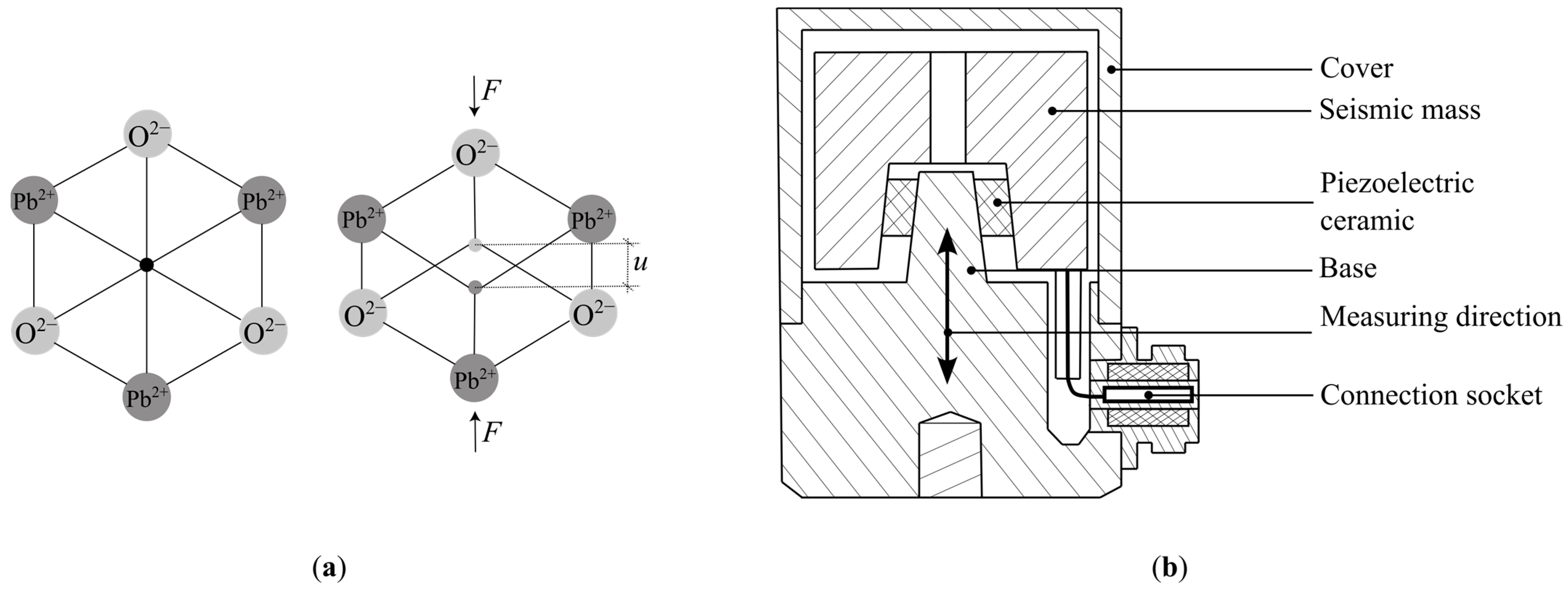
2.1. Measuring Principle

The IEPEs employed are based on the physics of piezo-electricity [33,34]. To elaborate, a piezoelectric ceramic made of lead zirconate titanate within the sensor deforms when subjected to a mechanical force F. This deformation results in an electrical voltage U. Figure 2 schematically illustrates the design of a piezoelectric accelerometer.
The left part of Figure 2 shows the principle of the piezoelectric effect with a piezoceramic made of lead zirconate titanate as an example. In an unstressed state, the centers of positive and negative charges coincide. In a stressed state, there is a shift u of the charge centers, leading to an electrical polarization, which can be measured as an electrical voltage U. Furthermore, the applied acceleration can be directly inferred using Newton’s second law F = m · a , [35]. It is important to note that the piezoelectric effect can only occur in non-conductive materials without a center of symmetry [36]. The right part of Figure 2 shows the principal structure of the IEPE sensor being investigated, which is designed as a so-called ‘shear system’. The sensor consists of two components, the piezoelectric ceramic and a seismic mass. The combined components form a spring-mass system with one degree of freedom [37,38]. Compared to other IEPE sensor designs, such as ‘compression’ or ‘bending systems’, the IEPE shear sensor represents a compromise between sensitivity, robustness, and susceptibility to interference for acceleration measurements. It is the most commonly used design of IEPE sensors for measuring engineering structures [39]. This study focuses on the analysis of the transmission behavior of this sensor type in the low-frequency range. However, it is important to note that other IEPE design types (compression or bending systems) may show different behavior under the influence of environmental factors. This shall be taken into account when designing IEPE-based measurement systems.

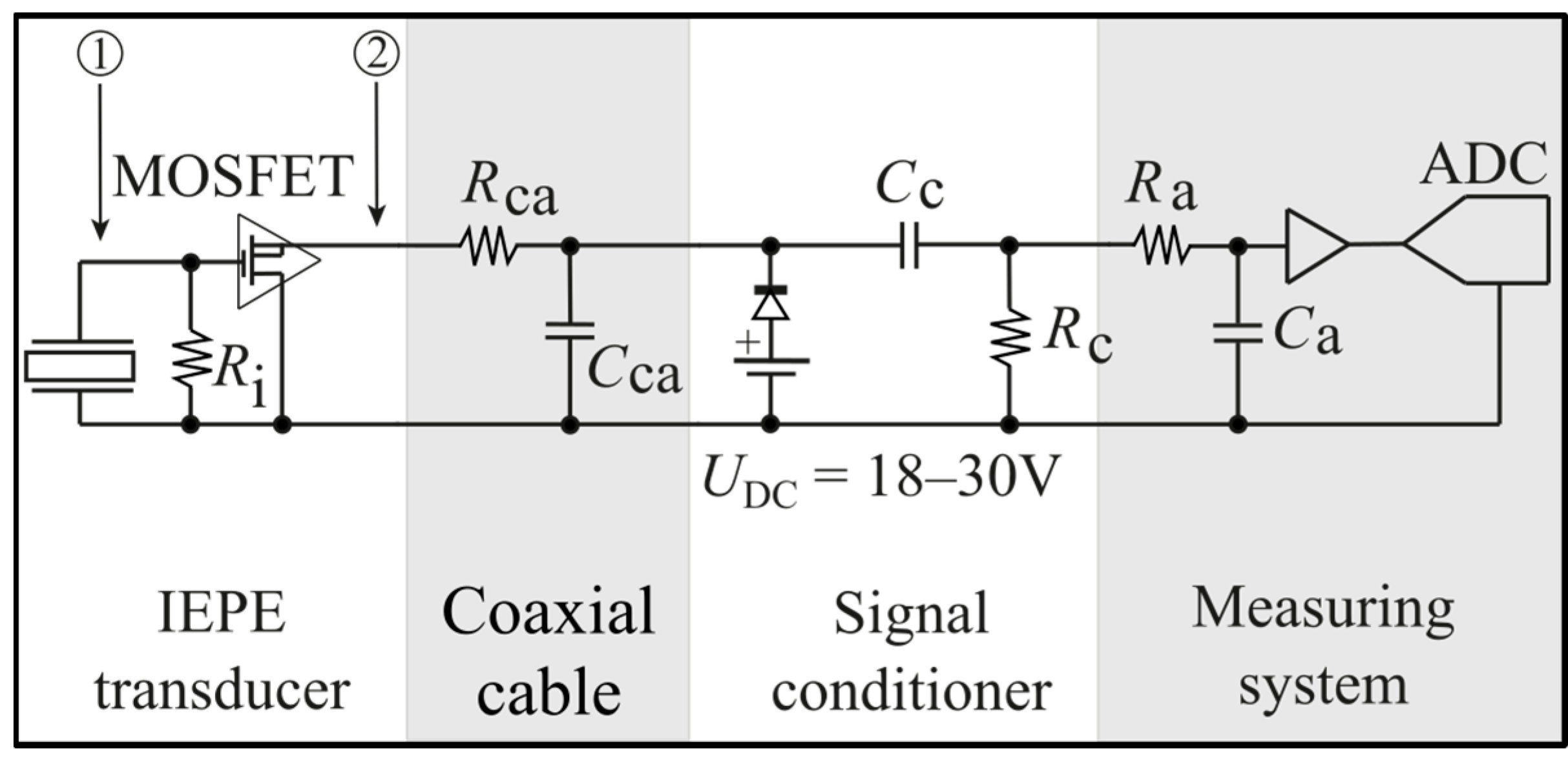
2.2. Signal Conditioning

The IEPE measurement chain used in this paper is schematically shown in Figure 3. It is assumed that the entire measurement chain is a linear, time-invariant system. In this context, ‘linearity’ means that the output signal is proportional to the input signal. In this case, a sinusoidal input signal of a given frequency also generates a sinusoidal output signal of the same frequency. Nevertheless, the amplitude and phase may differ as a function of the frequency. ‘Time invariance’ means that the output signal will respond consistently to the input signal at any given time, regardless of the specific point in time [40]. However, the ‘time invariance’ assumption is questioned because environmental influences can affect the measurement system over time due to aging. This time-variant behavior of measurement systems can be observed, for instance, in [30].
The measurement chain consists of an IEPE transducer, a coaxial cable, a signal conditioner, and a measuring system. The IEPE transducer is a two-wire system (input and output) and has an integrated amplifier, which is an impedance converter implemented as a MOSFET (Metal Oxide Semiconductor Field-Effect Transistor) circuit. The MOSFET enables high-impedance voltage signals to be amplified to low-impedance voltage signals. This leads to significantly better noise performance and less loss of signal quality [24]. Due to this low-loss signal transmission, inexpensive coaxial cables, which may be several hundred meters long, can be used without concerns about losing the quality of the measurement signal, such as increased noise or susceptibility to environmental factors [41]. In current research, there are also approaches using wireless acceleration sensors. For instance, Xie et al. developed a passive accelerometer employing an unstressed patch antenna for data acquisition [42]. Hidalgo et al. presented a wireless and low-power system for structural damage assessment [43]. However, wireless measurement systems are not studied here because they are not the standard use case in engineering fields. The signal conditioner, as the next measuring chain component, is composed of a DC voltage source and a current-regulating diode, which are responsible for a constant current supply to the IEPE transducer via the coaxial cable [41]. The constant current supply to the IEPE transducer generates a positive bias voltage, which is U Bias = 13   V for the IEPE sensor used. This bias voltage is separated from the actual raw data signal by the coupling capacitor Cc. The combination of the coupling capacitor Cc and load resistor Rc forms a first-order high-pass filter whose lower cutoff frequency is given by Equation (1):
f u = 1 2 π R c C c
Hence, the measurable lower frequency limit of the accelerations depends on the signal conditioner and the sensor. According to the datasheets, the used sensor and signal conditioner have a lower cut-off frequency of 0.1 Hz, which is sufficient for the planned study in this paper and practical applications, e.g., wind turbines [44].
As the last component of the measurement chain, the measuring system contains an analog-to-digital converter (ADC) that converts the analog voltage signal into a digital signal with a sufficiently high sampling frequency. Additionally, the capacitor Ca and resistor Ra form a low-pass anti-aliasing filter so that interfering noise signal components are filtered out of the raw data signal, and a digital, time-discrete measurement signal is generated for further processing.
The measurement module used was manufactured by GANTNER INSTRUMENTS; it includes both the signal conditioner and the measuring system. The used Q.bloxx XL A111 measuring module is specially designed for measuring IEPE sensors, and the transmission behavior is shown in Table 1.
The cut-off frequency of the measuring module, i.e., the frequency at which the amplitude of the output signal reaches only 70.7% (−3 dB) of the input amplitude [45], is 0.1 Hz. At 0.3 Hz, the ratio is 100% (no amplitude reduction). In the measuring module, the delta-sigma modulation with a sampling depth of 24 bits is employed for analog-to-digital conversion. The specifications of the components used show that the measuring chain is suitable for frequency ranges between 0.2 and 1.0 Hz, which is of interest in this study.

3. Sensor Calibration: Experimental Setup and Execution

This section presents the experimental setup to test the IEPE sensors. With this setup, a noise analysis was conducted. Furthermore, a reference measurement was conducted using a standardized calibration station at the Bundesanstalt für Materialforschung und-prüfung (BAM, in English: Federal Institute for Materials Research and Testing). Furthermore, the comparative measurement was carried out at the TU Dresden (TUD), Dresden, Germany. The main differences between the two test series are listed in Table 2.

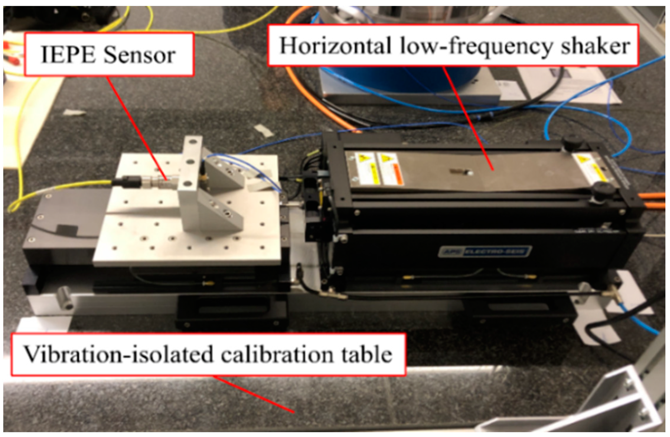
3.1. Experimental Setup of the Standardized BAM Calibration Station

The low-frequency calibration system at BAM facilitated the precise calibration of acceleration sensors according to DIN ISO 16063-21 [20]. This system is located on a calibration table which is decoupled from the foundation, effectively suppressing any external vibrations. The system comprises a horizontally oriented low-frequency shaker, upon which an air-cushion-supported sled is electromagnetically excited. The experimental setup is illustrated in Figure 4.
The metrology of this overall system is traceable to the calibration norm of the Physikalisch-Technische Bundesanstalt (in English: National Metrology Institute) in Braunschweig, Germany. The horizontal low-frequency shaker is capable of calibrating a test object of up to 23 kg in frequency ranges from 0.2 Hz to 200 Hz with a maximum possible stroke of 140 mm. The IEPE sensors to be examined must be able to reliably detect the first natural frequencies of wind turbines. Consequently, the low-frequency accelerations in the frequency range from 0.2 Hz to 1.0 Hz are of interest for this calibration. The peak accelerations achieved using the calibration system are presented in Table 3.

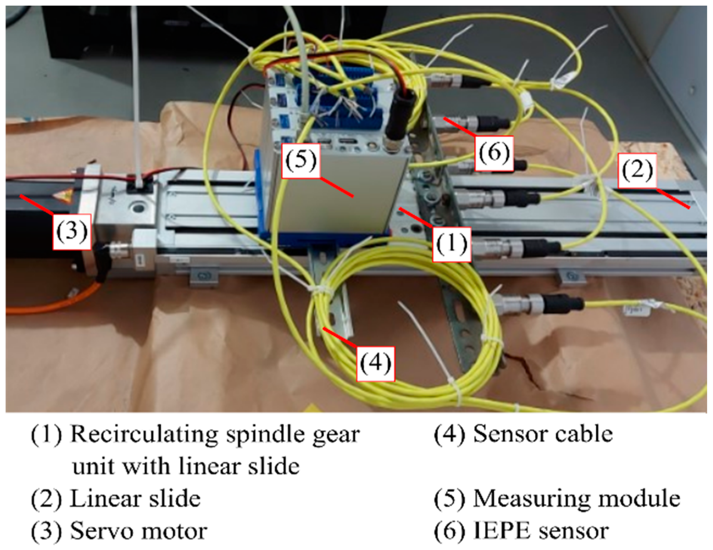
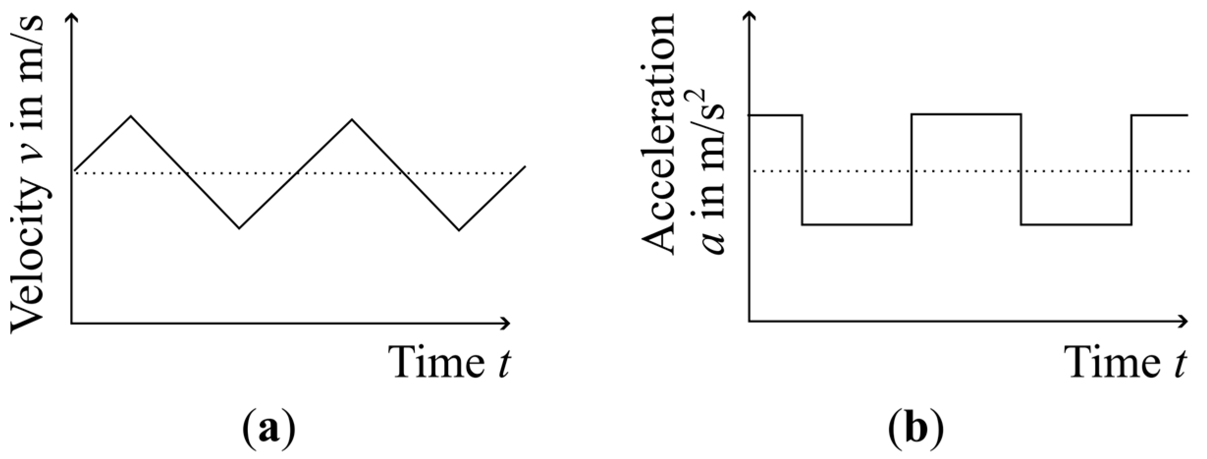
3.2. Experimental Setup of the Linear Unit
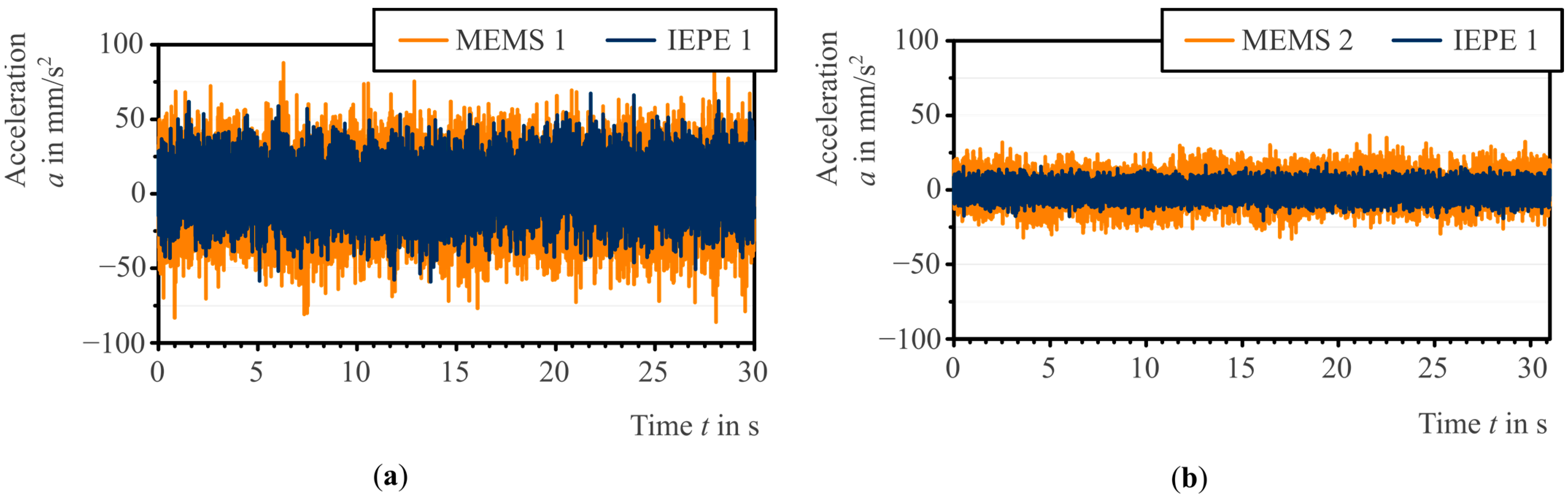
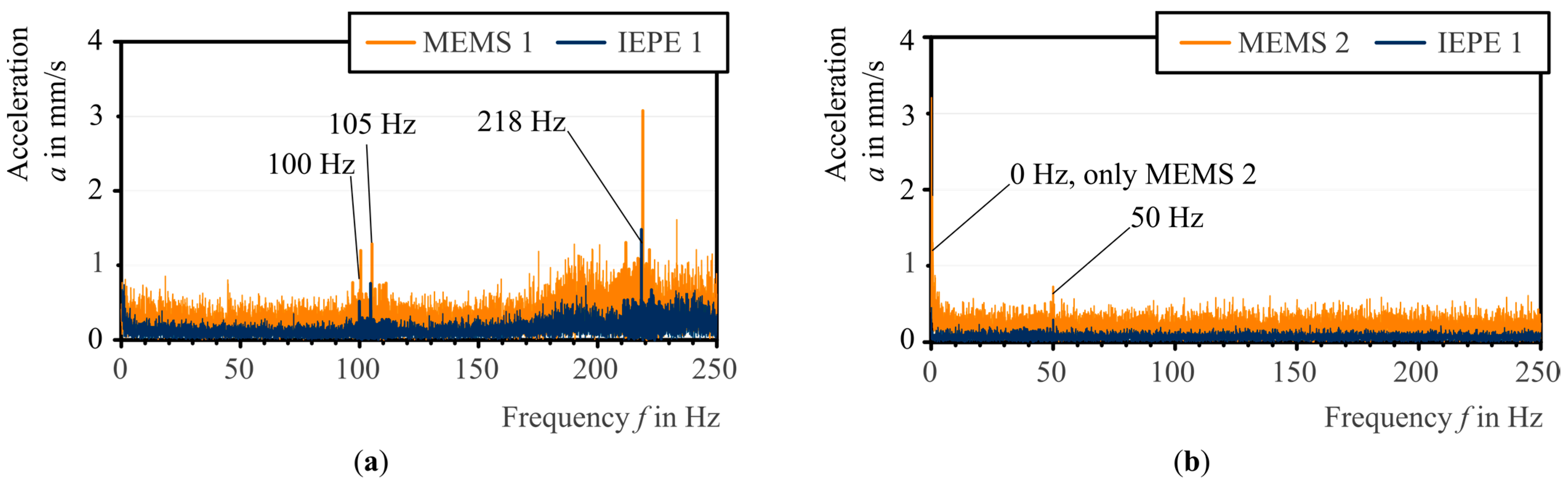
Since the BAM calibration system is stationary and unable to accommodate variations in environmental conditions inside a climate chamber, an alternative calibration station was set up inside a climate chamber at the Institute of Concrete Structures, TU Dresden, Dresden, Germany. The climate chamber has a test volume of 2.00 m × 2.00 m × 2.00 m. The chamber has a frequency-controlled refrigeration unit that can extract heat from the chamber using the frequency converter. An air cooler guarantees uniform air distribution and thus ensures a constant room temperature of up to −25 °C in every corner of the chamber. The chamber is supplemented by a tube heater that can heat the temperature to +100 °C. In addition to the temperature-regulating components, an ultrasonic humidifier and an adsorption dryer enable the relative humidity (RH) to be regulated from 25% RH to 85% RH. The climate chamber can be electronically controlled to program temperature and humidity cycles, making it easier to carry out regular analyses. Figure 5 shows the experimental setup installed in the climate chamber, which primarily consists of a linear unit that is commonly used in automation technology.
In this setup, the rotational motion of a servo motor is converted into translational motion through a spindle drive and drives a linear slide. By periodically changing the direction of rotation of the motor, an oscillating motion of the linear slide is generated. In this way, a stroke of up to 160 mm can be achieved. However, due to the limited controllability provided by the basic configuration of the linear unit, it is not capable of producing harmonic vibrations. The control software only supports linear velocity or constant acceleration profiles, as depicted in Figure 6.
The sensors and the measurement module were mounted on the linear slide to mitigate the noise levels in measurements that may result from the fraction of coaxial cables. By securing the components of the measurement chain, relative movements were avoided, effectively suppressing the undesired noise impact. Similarly, in the low-frequency calibration system at BAM, noise effects were mitigated by orienting the coaxial cable horizontally away from the system. This prevented vibrations caused by potential frictional interactions between the cables and the calibration table. The resulting accelerations using the linear unit at TUD corresponding to the respective excitation frequencies, with an amplitude of 160 mm, are listed in Table 3.
Calibrating the accelerometers with the linear unit by applying the acceleration profile, as shown in Figure 6 (on the right side), can be controversial. On the one hand, it does not correspond to the recommended sine, multisine, or noise excitation in accordance with DIN ISO 16063-21, 4.4 [20]. On the other hand, it is not possible to measure constant accelerations with the IEPE sensors due to the sensor specificity of the RC circuit principle (in contrast to the MEMS sensors). Nevertheless, this acceleration profile was used for the identification of systematic measurement errors shown in Section 4. Although it does not adhere to the standard boundary conditions for the aforementioned calibration, it offers signal reproducibility, allowing for a qualitative evaluation of systematic influences from environmental factors.
To investigate the influence of temperature and relative humidity on the measurement signal, the experimental setup was assembled inside a climate chamber. However, before analyzing the impact of different environmental conditions on the measurement signal, it was necessary to carry out a noise analysis.

3.3. Noise Analysis

The noise behavior of the IEPE sensors was analyzed and compared with that of the MEMS sensors. Within the climate chamber at TUD, the MEMS sensor labeled as “MEMS 1” was employed for comparative purpose alongside the IEPE sensor. Additionally, the sensor “MEMS 2” at BAM, which was affixed to the calibration station, served as a reference sensor. Detailed specifications and characteristics of the utilized sensors can be found in Table 4.
A total of 20 measurements were recorded. Each measurement had a duration of 30 s and was sampled at a rate of 500 Hz. A comparison of the time-domain signals is illustrated in Figure 7.
The output signal of the IEPE 1 sensor (represented in blue color) tested in the climate chamber at TUD exhibited a significantly higher variation compared to the identical IEPE 1 sensor tested at BAM. This can be attributed to the less-noisy environment in the BAM facility, which is located on a vibration-isolated, heavyweight individual foundation. It can effectively dampen external influences, such as the vibrations from the Berlin subway system. In contrast, the experimental setup in the climate chamber at TUD is mounted directly on the floor without any additional isolation procedures, making it susceptible to external sources of vibration interference. Instances of potential disturbances include the operational vibrations stemming from the climate chamber’s refrigeration unit, as well as unidentified factors. Additionally, as observed in Figure 7, MEMS sensors (represented in orange color) exhibited higher noise compared to the IEPE 1 sensor. In the frequency spectra depicted in Figure 8, other differences can be observed.
In the spectrum of the noise signal generated in the climate chamber, clear peaks, such as those at 100 Hz, 105 Hz, and 218 Hz, could be observed, suggesting the presence of various external systematic influences. In contrast, the spectrum of the noise signal at BAM exhibited only the current noise at 50 Hz (typical mains hum in Germany due to the alternating current frequency of 50 Hz) and a separate peak of MEMS 2 at 0 Hz. The latter observation indicates that MEMS 2 was not precisely oriented horizontally concerning the direction of motion and, therefore, measured a part of the gravitational acceleration in this direction. For the sensor calibration at BAM, which is discussed in the following section, MEMS 2 was thus adjusted to the exact horizontal orientation.
In practice, it is usually recommended to use a sensor with higher sensitivity and lower noise density to reliably measure low-frequency accelerations in engineering structures. Table 4 shows the differences between the MEMS and IEPE sensors. On the one hand, the sensitivity of the MEMS sensors was higher than that of the IEPE sensors. On the other hand, the noise density of the MEMS sensors was significantly higher than that of the IEPE sensors. The comparison between MEMS 1 and IEPE shows that the sensitivity-to-noise density ratio was 250, while this ratio was 44 for MEMS 1. An acceleration sensor with a high sensitivity-to-noise density ratio should therefore be selected to reliably detect low-frequency vibrations on engineering structures. To investigate other influences in the low-frequency acceleration range, such as the frequency itself, the temperature, and humidity dependence, the sensors were subjected to motion using the calibration station and the linear unit.

3.4. Reference Measurement with Standardized Calibration Station

The experimental setup described in Section 3.1 was employed to perform the calibration of acceleration sensors according to DIN ISO 16063-21 [20], using a comparison with a reference transducer. The raw data signal of MEMS 2 and IEPE 1 at a frequency of 1 Hz, 20 °C temperature, and 50% RH is shown in Figure 9.
It can be seen that the amplitude U of the MEMS 2 sensor (approx. 200 mV) was greater than that of the IEPE 1 sensor (approx. 130 mV). This can be attributed to the higher sensitivity of the MEMS 2 sensor. Based on the amplitude of the IEPE 1 sensor, the frequency response can be determined, whereby the reference frequency is defined as 1 Hz. Additionally, a vibration acceleration of 2.571 m/s2 (see Table 3) is generated using the horizontal low-frequency shaker. Subsequently, the sensitivity S is calculated using Equation (2):
S = U a .
S is determined for different frequencies so that the frequency-dependent transmission behavior of the IEPE sensors can be evaluated via Equation (3) using the transmission factor TF (f):
T F ( f ) = S ( f ) S ( f = 1   Hz ) .
Figure 10 shows the result of four calibrated IEPE sensors in comparison to the reference transducer MEMS 2.
For each IEPE sensor, the number of oscillation periods per frequency was increased until at least six consecutively measured amplitudes per frequency had a standard deviation of less than 0.3% (accuracy of the BAM calibration station). This led to a calibration time of at least 30 min for a single sensor.
The left diagram in Figure 10 shows the non-linear transmission behavior of all four IEPE sensors compared to the linear transmission behavior of the MEMS 2 sensor. Additionally, the sensitivity of the sensor decreased as the frequency decreased. At the low-frequency oscillation of 0.2 Hz, the signal amplitude dropped by 5.5% to 8.5% compared to the signal at 1 Hz. At 0.3 Hz, there was only a 2.5% to 3.5% drop in the signal amplitude, whereas at 0.7 Hz, the signal no longer showed a significant drop. Furthermore, as the frequencies increased from 0.7 Hz to 1.0 Hz, the signal was attenuated by a maximum of 0.1% compared to the 1 Hz sensitivity. The right diagram in Figure 10 shows that the phase shift increased as the frequency decreased. At 0.2 Hz, a phase shift of up to 20° can be seen. This shift tended to approach a 0° phase shift with an increase in frequency up to 1 Hz. The phase shift, as the temporal displacement between the reference transducer MEMS 2 and the IEPE transducer, is especially considered in modal analyses of structures where multiple accelerometers are used for system identification (eigenfrequencies and eigenmodes), as discussed in [39]. The calibration was performed from 0.2 Hz to 10 Hz. However, since the amplitude response did not change significantly from 0.7 Hz (i.e., there was no obvious drop or gain in the signal amplitude), Figure 10 only shows the frequency response from 0.2 Hz up to 1.0 Hz.
This result is advantageous for bridges with typical natural frequencies from 2 Hz to 5 Hz. In comparison, it is essential to consider the sensitivity drop and the phase shift in the data normalization using the transfer function for wind turbines, which typically have eigenfrequencies ranging from 0.2 Hz to 1.0 Hz.

3.5. Comparison with a Simplified Calibration Unit

Following the procedure described in Section 3.4, the frequency response of the IEPE sensors was determined using the linear unit described in Section 3.2. The reason for employing this experimental setup is its capability to be installed in a climate chamber, enabling exposure to different temperatures and humidity levels for further investigation. Figure 11 illustrates the time-domain signal at a frequency of 1 Hz.
A Bessel low-pass filtering technique was employed in this case to illustrate the signal quality. Unlike the BAM calibration station, the linear unit did not generate harmonic vibrations. The qualitative acceleration profile as an input signal, shown in the right diagram of Figure 6, can be transferred in the time domain as an output signal from the MEMS 1 sensor in Figure 11. The time-domain signal from the IEPE 1 sensor exhibited a voltage decay over time, even when the acceleration remained constant according to the reference transducer. This behavior is due to the functionality of the IEPE sensor. Unlike MEMS sensors, IEPE sensors cannot measure constant accelerations. They possess an internal time constant, which approximately corresponds to a first-order RC high-pass filter. As a result, when subjected to a step input, the sensor responds with an exponentially decaying amplitude. Regarding the reproducibility of the results, it is important to select an amplitude for the IEPE signal that occurs at the time of the constant acceleration range. In Figure 11, the peak amplitude per oscillation is therefore used, i.e., the IEPE signal at the start of the decay process. This procedure is important because otherwise the influences on the IEPE measurement system cannot be systematically compared regarding the environmental influences and frequency behavior. To quantify systematic temperature and humidity influences, a specific frequency (see Table 3), a specific temperature (−10 °C, 20 °C, or 50 °C), and a specific relative humidity (30% RH, 50% RH, or 80% RH) were kept constant for each IEPE sensor so that a total of 45 measurements were carried out for each sensor (1 Hz, 20 °C, and 50% RH was the reference measurement). Each measurement had a duration of twelve minutes and was sampled at 100 Hz. At least six consecutively measured amplitudes per frequency were selected for the data analysis. It is important to note that the initial two-minute transient process at the beginning of each measurement was excluded from the analysis, as otherwise, the transient behavior of the IEPE sensor would lead to a distorted analysis. The transmission behavior of the IEPE sensors was then calculated using Equations (2) and (3). Since the input signal per frequency was identical for each variation of the ambient condition, a valid analysis of the measuring system behavior for systematic temperature and humidity influences is possible.

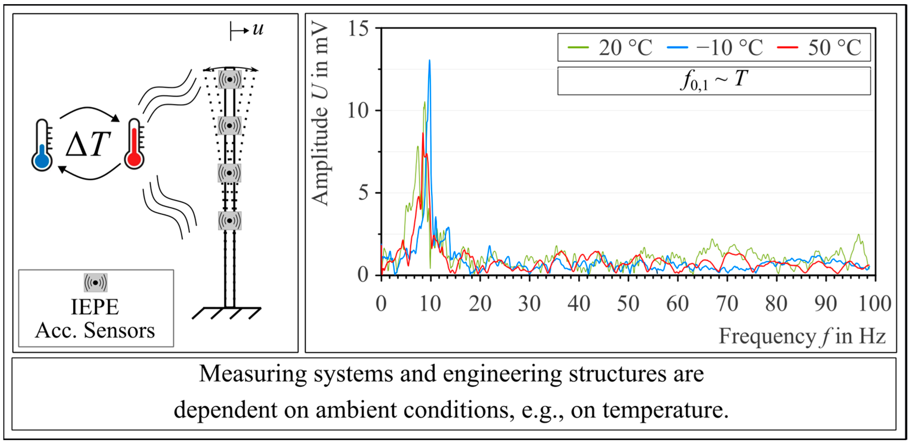
4. Systematic Environmental Influences on the IEPE Frequency Response

In the next step, the influence of temperature and relative humidity on systematic errors in the frequency response was investigated. The reference sensitivity for the IEPE sensor was determined with the conditions of a 1 Hz frequency, 20 °C temperature, and 50% relative humidity.

4.1. Temperature Influence on IEPE Frequency Response

To determine the temperature dependence of the frequency response, the temperature was varied within the climate chamber during the calibration process. To exclude possible systematic temperature influences on the linear unit, the stepper motor was equipped with a servo controller that included an oscilloscope function for measuring the dynamic excitation. In addition, redundant control measurements were performed using laser distance sensors, which ensured temperature-independent measurement of the dynamic excitation. For the distance measurement, the laser distance sensor was attached to a fixed point at the end of the linear unit, which was decoupled from the linear unit. The linear slide shown in Figure 5 moved during calibration and the laser distance sensor attached to the fixed point measured the change in distance over time. In both cases, a systematic temperature influence on the linear unit could be excluded. An analysis of the temperature influence on the phase shift could not be performed in this investigation, since the control measurements using oscilloscope and laser measurements were not digitized. Therefore, the evaluation was limited to the frequency response. The results for two IEPE sensors are shown in Figure 12.
A temperature change of 30 °C (from −10 °C to 20 °C, or from 20 °C to 50 °C) led to a change in the frequency response of both IEPE sensors; the sensitivity of IEPE sensors increases as the temperature increases. The temperature dependence can be explained by the material properties of the piezoelectric lead zirconate titanate ceramic used, which are defined by piezoelectric material constants. The coefficients can be derived from the mechanical–thermodynamic material behavior of the ceramic. The coefficients can be determined according to DIN EN 50324-2:2002-12 [46] and described via the linear equations of state of an elastic dielectric with piezoelectric properties [37,46,47].
Based on this result, it can be concluded that temperature changes impact the sensitivity of the measurement system. This knowledge is already stated generally in the sensor manufacturers’ data sheets. For the IEPE sensors used, there was a 10% reduction in sensitivity at −25 °C and a 15% increase in sensitivity at +120 °C [44]. However, these calibration certificates are valid for a frequency range of 5 Hz to 10 kHz, which means that IEPE calibration certificates are no longer suitable for use in the construction industry. The analysis carried out in this paper shows that a systematic temperature dependence must also be taken into account for typical boundary and ambient conditions in the construction industry; otherwise, damage to the structure cannot be distinguished reliably from the varying system behavior of the sensors.

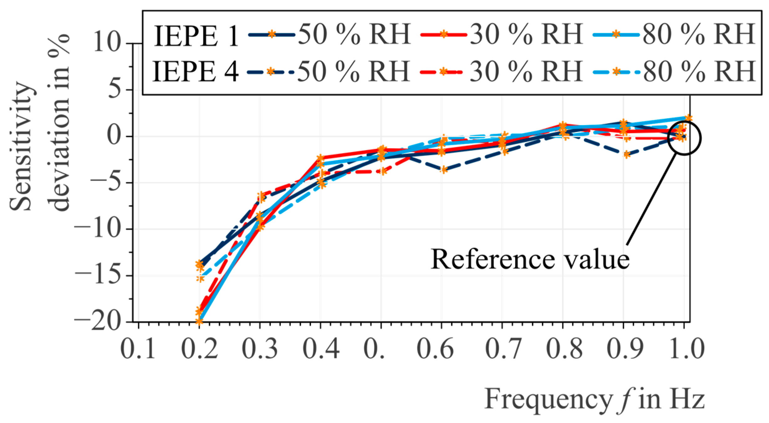
4.2. Air Humidity Influence on IEPE Frequency Response

In addition to the first series of experiments described in Section 4.1, a second series of experiments was conducted to investigate the influence of relative humidity on the frequency response of IEPE sensors. The results for two IEPE sensors exposed to varying relative humidity levels of 30%, 50%, and 80% are depicted in Figure 13.
Compared to the observed temperature dependency of the frequency response, a variation in relative humidity did not produce a significant change in the frequency response. Only at a frequency of 0.2 Hz was a significant change at different humidity levels visible. Under humid (80% RH) and dry (30% RH) conditions, the sensitivity at 0.2 Hz was up to 4% lower than that under moderate humidity conditions (50% RH). This observation should be critically assessed because no systematics were visible at other frequencies. The result can be attributed to a degree of uncertainty in the test procedure. Nevertheless, the independence of the sensitivity from humidity at frequencies of 0.3 Hz to 1.0 Hz can be attributed to the hermetic sealing of the sensor electronics within the sensor case, which protects against dust and moisture ingress.

5. Case Study

To validate the calibration results from Section 3 and Section 4 as well as to separate the sensor behavior from the structural behavior, the IEPE sensors were mounted on a small-scale support structure. The experimental setup including data analysis is described and discussed in the following.

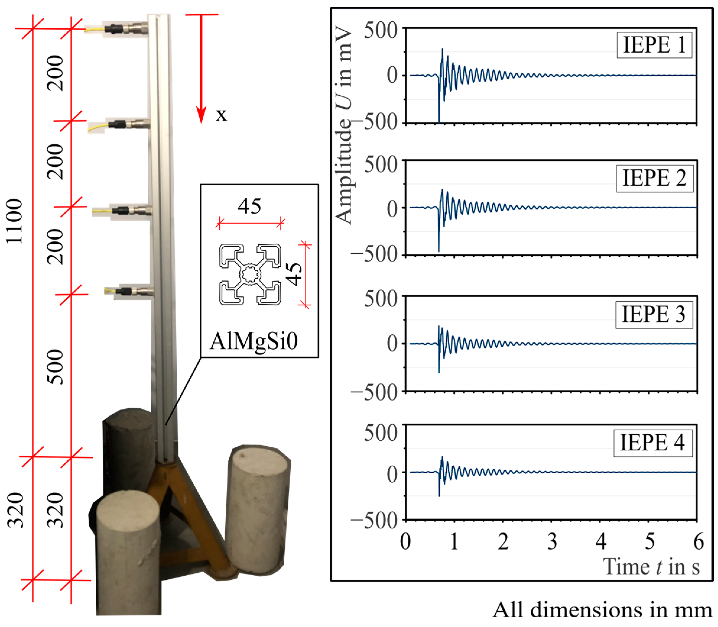
5.1. Experimental Setup and Data Acquisition

Figure 14 shows the experimental setup, which is a clamped vertical cantilever beam similar to the tower structure of a wind turbine. The experimental setup was set up inside the climate chamber and was exposed to different temperatures to separate the behavior of the IEPE sensor from the behavior of the engineering structure. The raw data signals of the four IEPE sensors for one swing-out test are also depicted in Figure 14.
The beam was 1.10 m long and made of a rectangular aluminum profile (AlMgSiO); the cross-sectional dimensions were 45 × 45 mm. The beam was connected to a three-leg base construction using bolts, and the three legs were fixed with concrete weights to establish a situation of rigid clamping. Starting from the free end of the cantilever beam, four IEPE sensors with a distance of 20 cm and coordinates of x = [0 cm; 20 cm; 40 cm; 60 cm] in the x-axis direction were installed using bolted connections. The sensor properties are listed in Table 4. During the tests, the measurement signal was captured at a frequency of 200 Hz.
To examine the dynamic response of the structure and the sensors, a swing-out of the system was induced by displacing the cantilever’s head by 2.80 mm ± 0.10 mm. Additionally, to quantify the dynamic response of the IEPE sensors, a parallel comparative measurement was executed using a laser triangulation sensor, which measured the deflection of the cantilever throughout the complete experimental duration. Previous studies show that temperature does not affect the frequency response of laser triangulation measurements, so an accurate reference for evaluating IEPE behavior can be ensured [30]. For the distance measurement, the laser distance sensor was attached to a fixed point at the free end of the cantilever beam, which was decoupled from the structure. With this configuration, the sensor measured the change in distance over time and the signal could be compared to the IEPE signal. In addition, a damage simulation was conducted through the implementation of a mass alteration. This was achieved by attaching individual masses to the structure at specific positions, x = [10 cm; 30 cm], each weighing 0.22 kg. Consequently, a mass change of 3% or 6% was simulated, considering that the weight of the structure was 7.30 kg. A change in mass in this percentage order of magnitude is not realistic for real engineering structures, even if there are permanent traffic loads (e.g., due to traffic jams) or other external influences such as wind acting on the structure. However, in this case study, the intention was to compare the variation in the measurement signal caused by damage with the variation in the measurement signal caused by temperature changes.
To investigate the behavior of the structure and the sensor at different temperatures, the test setup was subjected to the same deflection and thus the same oscillation process four times each at temperatures of T = [−10 °C; 20 °C; 50 °C], with the relative humidity held constant at 50%.

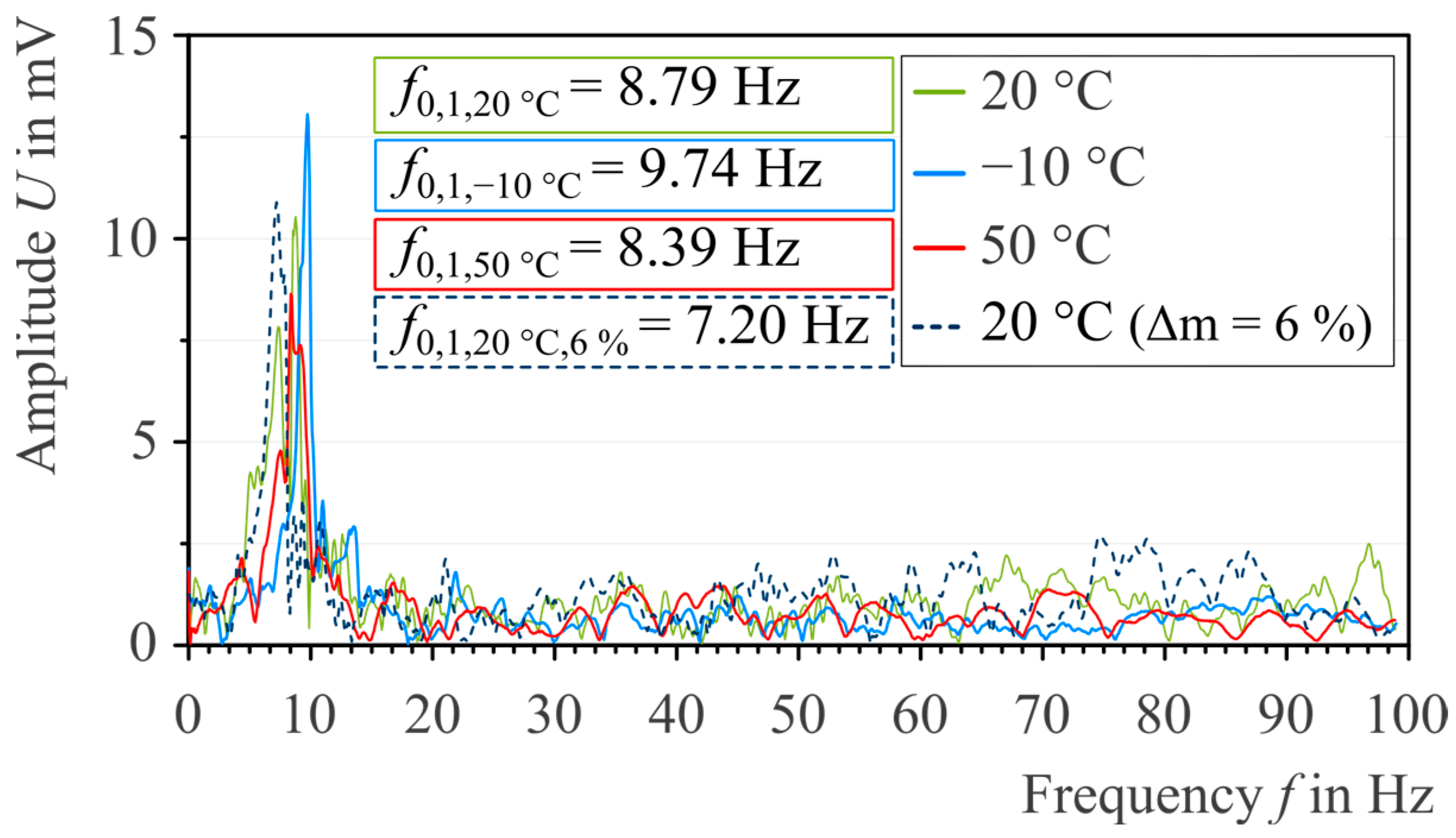
5.2. Data Analysis and Evaluation with Signal Energy Method

Fast Fourier Transformation (FFT) was used to compare the measurement signals with different features. Figure 15 displays the frequency space representation of the IEPE 1 signal.
Based on this, the initial modal eigenfrequencies f0,1 of the structure at −10 °C, 20 °C, 50 °C, and 20 °C with a 6% increase in mass can be confidently determined. The temperature showed an obvious impact on the eigenfrequencies of the system. For instance, a temperature reduction of 30 °C, from 20 °C to −10 °C, resulted in an 11% increase in f0,1 from 8.79 Hz to 9.74 Hz, whereas an increase in temperature of 30 °C, from 20 °C to 50 °C, resulted in a 5% decrease in f0,1 to 8.39 Hz. These results indicate a significant influence of temperature on the dynamic behavior of the structure. The reason for this behavior is that the temperature can influence the stiffness of the aluminum beam. Studies [48,49,50] show that a structure’s stiffness increases as the temperature decreases, resulting in an increase in the eigenfrequency.
Additionally, it can also be seen that the f0,1 was 7.20 Hz at 20 °C with a 6% mass change, leading to an 18% shift in the eigenfrequency. A 6% change in mass resulted in a much more significant change in natural frequency compared to the changes generated by temperature variations. However, smaller system changes and damages are likely to be expected in practice, while the temperature gradients are realistic. This shows it is evident to consider environmental conditions in the data analysis procedure.
To differentiate the behavior of the sensor from the supporting structure, a comparison of the accelerometer and laser triangulation sensor measurements was conducted. Table 5 provides the essential data for this case study, featuring columns that highlight IEPE 1 and IEPE 4—two previously examined sensors. The first modal eigenfrequency f0,1 and the relative signal energy Erel (see Equation (5)) for the sensors under varying temperatures and mass changes were determined.
To distinguish the sensor’s behavior from the global structural behavior, a new evaluation parameter was established. An analysis of the swing-out process in the time domain was conducted to evaluate the sensor performance under various temperatures. This involved calculating the signal energy of the time signal. Since the laser triangulation sensor displayed consistent frequency behavior under different temperatures, T, it served as the reference point against which the signal energy obtained from the IEPE sensor was compared. The recorded signals from both the laser triangulation sensor and the IEPE sensors were stored as time-discrete sequences. The signal energy of a time-discrete signal x [n] was defined as the summation of the squared magnitudes of all its samples in the time domain [49,51] and can be calculated as
E = n = 1 N x n 2 ,
where x [ n ] denotes the magnitude of the n-th sample point and N represents the number of samples. The signal energy describes the strength of the signal within a defined period [50], and can thus reflect the measured signal quality of the sensors. To evaluate the influence of the temperature on the IEPE sensors separately, the structure response, which is measured by the laser triangulation sensor, shall be excluded. This is achieved by utilizing the measurement obtained from the laser triangulation sensor as a reference value. Subsequently, the relative energy Erel is calculated using Equation (5)
E r e l = E I E P E E L a s e r .
It is important to note that the laser triangulation sensor and IEPE sensors measured different physical properties, namely displacement and acceleration. Hence, their signal energies are associated with different units: the signal energy of the laser triangulation sensor is expressed in mm2, while the signal energy of IEPE sensors is quantified in mV2.
By using the parameter Erel, the observation made during the calibration procedure (Section 4) can be confirmed qualitatively. The temperature affected not only the support structure but also the sensor behavior. When the temperature was higher than 20 °C, the signal energy ratio between the IEPE sensor and the laser triangulation sensor also increased for every tested sensor and vice versa, as depicted in Table 5 for both IEPE 1 and IEPE 4. This was further confirmed by the experiments where the mass was changed rather than the temperature, as there was a much smaller change in the signal energy ratio. Hence, it can be confidently stated that temperature changes significantly influence the sensitivity of the IEPE sensor within the complex overall system, which includes both the sensor and the structure, and this systematic error should be compensated for in the overall data analysis of engineering structures with low-frequency accelerations.

6. Discussion and Outlook

This paper investigated the transmission behavior of acceleration sensors within the low-frequency range under varying conditions. The focus was on IEPE sensors, which are suitable for measuring low-frequency vibrations in SHM applications for engineering structures. The results can be summarized as follows:
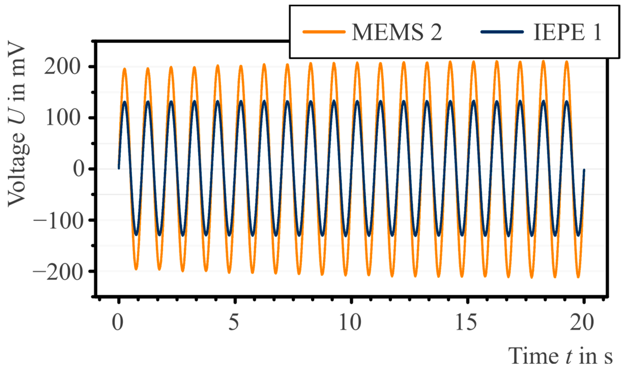
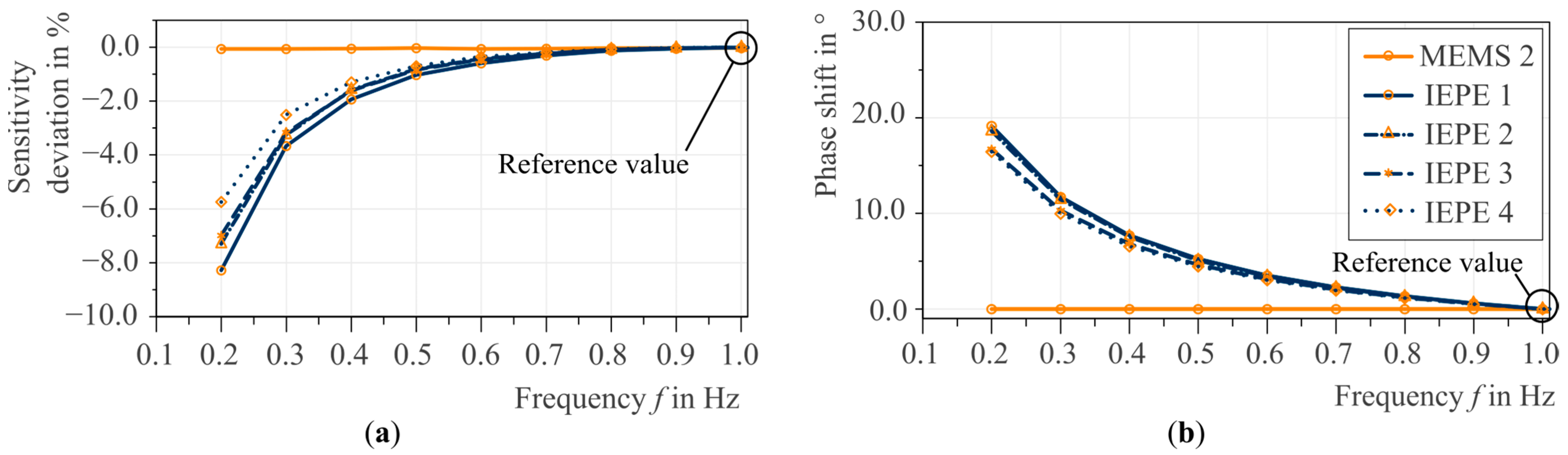
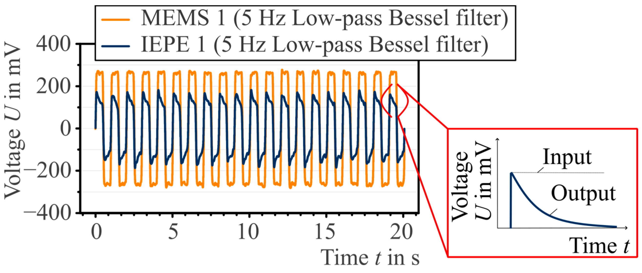
  • IEPE sensors have a non-linear transmission behavior, which ideally must be determined by sensor-specific calibration using a horizontal low-frequency shaker. MEMS sensors have the advantage of linear transmission behavior; however, a significant disadvantage of MEMS sensors is the high noise level. Thus, IEPE sensors are recommended for low-frequency acceleration measurement in engineering fields.
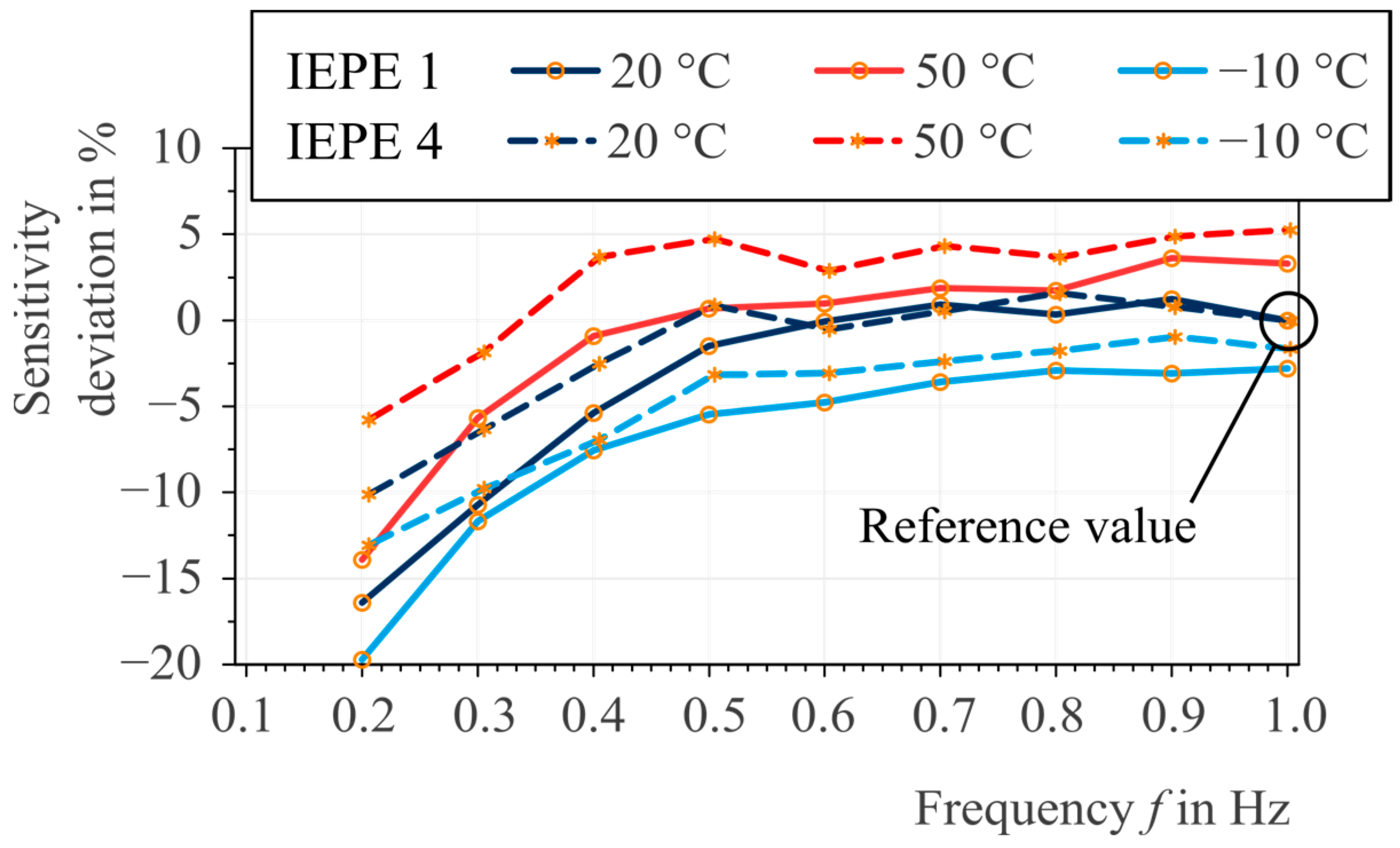
  • Due to the temperature dependency of the piezoelectric constants, the transmission behavior of IEPE sensors in the low-frequency range is temperature-dependent. The sensor sensitivity increases with rising ambient temperatures. Within the temperature range of −10 °C to +50 °C, there was a deviation in sensitivity of up to 10%, independent of the tested frequency range of 0.2 Hz to 1.0 Hz.
  • Based on the test results—although there was some uncertainty in the test procedure—the transmission behavior of IEPE sensors in the low-frequency range can be interpreted as almost independent of the air humidity.
  • In the case study, it was demonstrated that, for a precise measurement-based evaluation of structural behavior, both the sensor response and the structural response should be assessed separately. For this, parameters like signal energy can be suitable for evaluation features.
The compensation of systematic influences on the structure and on the sensor system, such as temperature, is essential for a robust SHM. In practice, there is a risk that the measurement signal may be obscured by measurement noise at low temperatures due to low sensitivity and high noise density. To mitigate this, it is advisable to select an accelerometer with high sensitivity (e.g., 500 mV/g) and low noise density (e.g., 2   µ g / Hz ). Furthermore, IEPE sensors may underestimate the response of the supporting structure at low temperatures and overestimate it at higher temperatures. In many practical cases, only the frequency within the spectrum is of interest; however, there are also instances where, for example, the dynamic magnification factor is calculated based on vibration energy, resulting in a static equivalent force. In such cases, actual measurements at lower temperatures could lead to an underestimation of the vibration energy E r e l and, consequently, to an underestimation of the static equivalent force (e.g., earthquake engineering). Therefore, it is essential in practical applications to account for these influences to reduce potential sources of sensor error. The selection of IEPE sensors with minimal temperature dependence and precise data normalization of the raw data is still crucial to improve the reliability of SHM.

Author Contributions

Conceptualization, J.-H.B. and R.H.; methodology, J.-H.B. and R.X.; software, J.-H.B. and R.X.; validation, J.-H.B.; formal analysis, J.-H.B.; investigation, J.-H.B.; resources, J.-H.B.; data curation, J.-H.B.; writing—original draft preparation, J.-H.B. and R.X.; writing—review and editing, J.-H.B., C.K. and R.H.; visualization, J.-H.B.; supervision, S.M.; project administration, S.M.; funding acquisition, S.M. All authors have read and agreed to the published version of the manuscript.

Funding

This research was funded by the German Research Foundation (DFG), as part of the Collaborative Research Centre 1463 (SFB 1463) “Integrated Design and Operation Methodology for Offshore Megastructures” (subproject C01, project number 434502799), and by the German Federal Ministry for Economic Affairs and Climate Action (BMWK) [grant numbers: 03EE2025A]. This article represents the opinions of the authors and does not mean to represent the position or opinions of the funding entities.

Data Availability Statement

The data presented in this study are available on request from the corresponding author.

Conflicts of Interest

The authors declare no conflicts of interest.

References

  1. Botz, M.; Oberlaender, S.; Raith, M.; Grosse, C. Monitoring of Wind Turbine Structures with Concrete-steel Hybrid-tower Design. In Proceedings of the 8th European Workshop on Structural Health Monitoring (EWSHM 2016), Bilbao, Spain, 5–8 July 2016; pp. 1–11. [Google Scholar]
  2. Orbán, Z.; Gutermann, M. Assessment of masonry arch railway bridges using non-destructive in-situ testing methods. Eng. Struct. 2009, 31, 2287–2298. [Google Scholar] [CrossRef]
  3. Proske, D.; Sykora, M.; Gutermann, M. Verringerung der Versagenswahrscheinlichkeit von Brücken durch experimentelle Traglastversuche. Bautechnik 2021, 98, 80–92. [Google Scholar] [CrossRef]
  4. Hafiz, A.; Schumacher, T. Monitoring of Stresses in Concrete Using Ultrasonic Coda Wave Comparison Technique. J. Nondestruct. Eval. 2018, 37, 73. [Google Scholar] [CrossRef]
  5. Rizzo, P.; Enshaeian, A. Challenges in Bridge Health Monitoring: A Review. Sensors 2021, 21, 4336. [Google Scholar] [CrossRef]
  6. Giagopoulos, D.; Arailopoulos, A.; Dertimanis, V.; Papadimitriou, C.; Chatzi, E.; Grompanopoulos, K. Structural health monitoring and fatigue damage estimation using vibration measurements and finite element model updating. Struct. Health Monit. 2019, 18, 1189–1206. [Google Scholar] [CrossRef]
  7. Omidalizarandi, M.; Herrmann, R.; Kargoll, B.; Marx, S.; Paffenholz, J.-A.; Neumann, I. A validated robust and automatic procedure for vibration analysis of bridge structures using MEMS accelerometers. J. Appl. Geod. 2020, 14, 327–354. [Google Scholar] [CrossRef]
  8. Shariati, A.; Schumacher, T. Eulerian-based virtual visual sensors to measure dynamic displacements of structures. Struct. Control Health Monit. 2017, 24, e1977. [Google Scholar] [CrossRef]
  9. Fremmelev, M.A.; Ladpli, P.; Orlowitz, E.; Dervilis, N.; McGugan, M.; Branner, K. A full-scale wind turbine blade monitoring campaign: Detection of damage initiation and progression using medium-frequency active vibrations. Struct. Health Monit. 2023, 22, 4171–4193. [Google Scholar] [CrossRef]
  10. Chen, S.; Cerda, F.; Rizzo, P.; Bielak, J.; Garrett, J.H.; Kovacevic, J. Semi-Supervised Multiresolution Classification Using Adaptive Graph Filtering with Application to Indirect Bridge Structural Health Monitoring. IEEE Trans. Signal Process. 2014, 62, 2879–2893. [Google Scholar] [CrossRef]
  11. Wenzel, H. Health Monitoring of Bridges, 1st ed.; John Wiley & Sons: Hoboken, NJ, USA, 2009; ISBN 9780470031735. [Google Scholar]
  12. Rolfes, R.; Zerbst, S.; Haake, G.; Preetz, J.; Lynch, J.P. Integral SHM-System for Offshore Wind Turbines Using Smart Wireless Sensors. In Proceedings of the 6th International Workshop on Structural Health Monitoring, Hong Kong, China, 9 December 2013; DEStech Publications Inc.: Stanford, CA, USA, 2007; pp. 11–13. [Google Scholar]
  13. Park, G.; You, D.; Oh, K.-Y.; Nam, W. Natural Frequency Degradation Prediction for Offshore Wind Turbine Structures. Machines 2022, 10, 356. [Google Scholar] [CrossRef]
  14. Fraden, J. Handbook of Modern Sensors: Physics, Designs, and Applications, 5th ed.; Springer: New York, NY, USA, 2016; ISBN 9783319193038. [Google Scholar]
  15. Aabid, A.; Parveez, B.; Raheman, A.; Ibrahim, Y.E.; Anjum, A.; Hrairi, M.; Parveen, N.; Zayan, J.M. A Review of Piezoelectric Material-Based Structural Control and Health Monitoring Techniques for Engineering Structures: Challenges and Opportunities. Actuators 2021, 10, 101. [Google Scholar] [CrossRef]
  16. Satija, J.; Singh, S.; Zope, A.; Li, S.-S. An Aluminum Nitride-Based Dual-Axis MEMS In-Plane Differential Resonant Accelerometer. IEEE Sens. J. 2023, 23, 16736–16745. [Google Scholar] [CrossRef]
  17. Anslow, R.; O’Sullivan, D. Choosing the Best Vibration Sensor for Wind Turbine Condition Monitoring. Analog. Dialogue 2020, 54, 1–6. [Google Scholar]
  18. Zanelli, F.; Debattisti, N.; Mauri, M.; Argentino, A.; Belloli, M. Development and Field Validation of Wireless Sensors for Railway Bridge Modal Identification. Appl. Sci. 2023, 13, 3620. [Google Scholar] [CrossRef]
  19. Bedon, C.; Bergamo, E.; Izzi, M.; Noè, S. Prototyping and Validation of MEMS Accelerometers for Structural Health Monitoring—The Case Study of the Pietratagliata Cable-Stayed Bridge. J. Sens. Actuator Netw. 2018, 7, 30. [Google Scholar] [CrossRef]
  20. DIN ISO 16063-21:2016-08; Verfahren zur Kalibrierung von Schwingungs- und Stoßaufnehmern—Teil 21: Schwingungskalibrierung durch Vergleich mit einem Referenzaufnehmer (ISO 16063-21:2003 + Cor. 1:2009 + Amd.1:2016). Beuth Verlag GmbH: Berlin, Germany, 2016.
  21. DIN EN ISO/IEC 17025:2018-03; Allgemeine Anforderungen an die Kompetenz von Prüf- und Kalibrierlaboratorien (ISO/IEC 17025:2017); Deutsche und Englische Fassung EN ISO/IEC 17025:2017. Beuth Verlag GmbH: Berlin, Germany, 2018.
  22. ISO 16063-21:2003-08; Methods for the Calibration of Vibration and Shock Transducers—Part 21: Vibration calibration by comparison with a reference transducer. Beuth Verlag GmbH: Berlin, Germany, 2013.
  23. Olivares, A.; Olivares, G.; Gorriz, J.M.; Ramirez, J. High-efficiency low-cost accelerometer-aided gyroscope calibration. In Proceedings of the 2009 International Conference on Test and Measurement (ICTM 2009), Hong Kong, China, 5–6 December 2009; IEEE: New York, NY, USA, 2009; pp. 354–360, ISBN 978-1-4244-4699-5. [Google Scholar]
  24. Jonscher, C.; Hofmeister, B.; Grießmann, T.; Rolfes, R. Very low frequency IEPE accelerometer calibration and application to a wind energy structure. Wind. Energ. Sci. 2022, 7, 1053–1067. [Google Scholar] [CrossRef]
  25. Bartels, J.-H.; Gebauer, D.; Marx, S. Einflüsse auf die Messunsicherheit von SHM-Systemen und deren Kompensation am Beispiel von Laser-Distanzmessungen. Bautechnik 2023, 100, 67–74. [Google Scholar] [CrossRef]
  26. Farrar, C.R.; Worden, K. Structural Health Monitoring: A Machine Learning Perspective, 1st ed.; John Wiley & Sons Incorporated: New York, NY, USA, 2012; ISBN 9781118443217. [Google Scholar]
  27. Peeters, B.; de Roeck, G. One-year monitoring of the Z24-Bridge: Environmental effects versus damage events. Earthq. Eng. Struct. Dyn. 2001, 30, 149–171. [Google Scholar] [CrossRef]
  28. Farrar, C.R.; Worden, K. An Introduction to Structural Health Monitoring. Philos. Trans. R. Soc. A 2007, 365, 303–315. [Google Scholar] [CrossRef]
  29. Viefhues, E.; Döhler, M.; Simon, P.; Herrmann, R.; Hille, F.; Mevel, L. Stochastic subspace-based damage detection of a temperature affected beam structure. In Proceedings of the 10th International Conference on Structural Health Monitoring of Intelligent Infrastructure, Porto, Portugal, 30 June–2 July 2021; pp. 1–6. [Google Scholar]
  30. Bartels, J.-H.; Kitahara, M.; Marx, S.; Beer, M. Environmental influence on structural health monitoring systems. In Life-Cycle of Structures and Infrastructure Systems, Proceedings of the Eighth International Symposium of Life-Cycle Civil Engineering (IALCCE 2023), Milan, Italy, 2–6 July 2023; Biondini, F., Frangopol, D.M., Eds.; CRC Press: Boca Raton, FL, USA, 2023; pp. 662–669. ISBN 978-1-003-32302-0. [Google Scholar]
  31. Stein, G.J. Some recent developments in acceleration sensors. Meas. Sci. Rev. 2001, 1, 183–186. [Google Scholar]
  32. Chalouhi, E.K.; Gonzalez, I.; Gentile, C.; Karoumi, R. Vibration-Based SHM of Railway Bridges Using Machine Learning: The Influence of Temperature on the Health Prediction. In Proceedings of the International Conference on Experimental Vibration Analysis for Civil Engineering Structures, Cham, Switzerland, 13 October 2018; Springer: Cham, Switzerland; pp. 200–211. [Google Scholar]
  33. DIN 1319-1:1995-01; Grundlagen der Meßtechnik—Teil 1: Grundbegriffe. Beuth Verlag GmbH: Berlin, Germany, 1995.
  34. Tuloup, C.; Harizi, W.; Aboura, Z.; Meyer, Y.; Khellil, K.; Lachat, R. On the use of in-situ piezoelectric sensors for the manufacturing and structural health monitoring of polymer-matrix composites: A literature review. Compos. Struct. 2019, 215, 127–149. [Google Scholar] [CrossRef]
  35. Nemirovsky, Y.; Nemirovsky, A.; Muralt, P.; Setter, N. Design of novel thin-film piezoelectric accelerometer. Sens. Actuators A Phys. 1996, 56, 239–249. [Google Scholar] [CrossRef]
  36. de Reus, R.; Gulløv, J.O.; Scheeper, P.R. Fabrication and characterization of a piezoelectric accelerometer. J. Micromech. Microeng. 1999, 9, 123–126. [Google Scholar] [CrossRef]
  37. Tichý, J.; Gautschi, G.H. Piezoelektrische Messtechnik: Physikalische Grundlagen, Kraft-, Druck-u. Beschleunigungsaufnehmer, Verstärker; Springer: Berlin/Heidelberg, Germany, 1980; ISBN 3540094482. [Google Scholar]
  38. Bigelow, H.; Pak, D.; Herrmann, R.; Schneider, S.; Marx, S.; Petraschek, T.; Feldmann, M.; Hoffmeister, B. Dynamische Messungen an einer Eisenbahnbrücke als Stahlbetonverbundrahmen. Stahlbau 2017, 86, 778–788. [Google Scholar] [CrossRef]
  39. Schneider, R.; Simon, P.; Hille, F.; Herrmann, R.; Baeßler, M. Vibration-based system identification of a large steel box girder bridge. In Eurodyn 2023; Metrikine, A., Ed.; TU Delft: Delft, The Netherlands, 2023. [Google Scholar]
  40. Oberst, U.; Scheicher, M.; Scheicher, I. Linear Time-Invariant Systems, Behaviors and Modules, 1st ed.; Springer International Publishing: Berlin/Heidelberg, Germany, 2020; ISBN 978-3-030-43935-4. [Google Scholar]
  41. Weber, M. Piezoelektrische Beschleunigungsaufnehmer: Theorie und Anwendung. Available online: https://www.mmf.de/manual/aufnehmerman.pdf (accessed on 10 May 2023).
  42. Xie, L.; Wu, T.; Yi, Z.; Fu, X.; Zang, W.; Lu, W. Passive Accelerometer Using Unstressed Patch Antenna Interrogated by FMCW Radar. IEEE Sens. J. 2023, 23, 16672–16682. [Google Scholar] [CrossRef]
  43. Hidalgo Fort, E.; Blanco-Carmona, P.; Garcia-Oya, J.R.; Muñoz-Chavero, F.; Gonzalez-Carvajal, R.; Serrano-Chacon, A.R.; Mascort-Albea, E.J. Wireless and Low-Power System for Synchronous and Real-Time Structural-Damage Assessment. IEEE Sens. J. 2023, 23, 13648–13658. [Google Scholar] [CrossRef]
  44. Althen Sensors & Controls 786LF Series Extremely Low-Frequency Accelerometer—Datasheet. Available online: https://www.althensensors.com/sensors/vibration-sensors/low-frequency-seismic-vibration-sensors/786-lf-low-frequency-seismic-vibration-sensors/ (accessed on 21 January 2024).
  45. Dorf, R.C. The Electrical Engineering Handbook—Six Volume Set; CRC Press: Boca Raton, FL, USA, 2018; ISBN 9781420049756. [Google Scholar]
  46. DIN EN 50324-2 VDE 0336-2:2002-12; Piezoelektrische Eigenschaften von Keramischen Werkstoffen und Komponenten. VDE Verlag: Berlin, Germany.
  47. Andreeff, A.; Fréederieksz, V.; Kararnosky, I. Die Abhängigkeit der piezoelektrischen Konstante bei Quarz von der Temperatur. Z. Phys. 1929, 54, 477–483. [Google Scholar] [CrossRef]
  48. Jones, D.R.H.; Ashby, M.F. Engineering Materials 1: An Introduction to Properties, Applications and Design, 5th ed.; Butterworth-Heinemann: Oxford, UK, 2019; ISBN 9780081020524. [Google Scholar]
  49. Große, C. Quantitative Zerstörungsfreie Prüfung von Baustoffen Mittels Schallemissionsanalyse und Ultraschall. Ph.D. Thesis, Universität Stuttgart, Stuttgart, Germany, 1996. [Google Scholar]
  50. Xu, R.; Hicke, K.; Chruscicki, S.; Marx, S. Akustisches SpRK-Monitoring mit SEA und verteilten faseroptischen Sensoren. In 12. Symposium Experimentelle Untersuchungen von Baukonstruktionen; TU Dresden: Dresden, Germany, 2023; pp. 136–147. [Google Scholar]
  51. Oppenheim, A.V.; Willsky, A.S.; Nawab, S.H. Signals and Systems, 2nd ed.; Prentice Hall: Upper Saddle River, NJ, USA, 1997; ISBN 0138147574. [Google Scholar]
Figure 1. An illustrative example of the dependence of the measuring system and the engineering structure on the environmental conditions using the example of the first modal eigenfrequency.
Metrology 04 00004 g001
Figure 2. Functionality of the IEPE sensor. (a) Measuring principle of a piezoelectric IEPE sensor; (b) design of an IEPE shear system.
Metrology 04 00004 g002
Figure 3. Electrical circuit diagram of the studied IEPE measurement chain.
Metrology 04 00004 g003
Figure 4. Calibration table and low-frequency shaker.
Metrology 04 00004 g004
Figure 5. Linear unit with mounted IEPE measuring chain.
Metrology 04 00004 g005
Figure 6. The achievable motion profiles with the linear unit (qualitatively). (a) Velocity profile; (b) acceleration profile.
Metrology 04 00004 g006
Figure 7. Comparison of noise behavior. (a) In the climate chamber; (b) in the 3rd basement floor of BAM.
Metrology 04 00004 g007
Figure 8. Frequency analysis. (a) In the climate chamber at TUD; (b) in the 3rd basement floor of BAM.
Metrology 04 00004 g008
Figure 9. Time signal at 1 Hz, 20 °C, and 50% RH.
Metrology 04 00004 g009
Figure 10. Calibration of the examined IEPE sensors at 20 °C and 50% RH. (a) Frequency response; (b) phase shift.
Metrology 04 00004 g010
Figure 11. Low-pass filtered time signal at 1 Hz, 20 °C, and 50% RH.
Metrology 04 00004 g011
Figure 12. Temperature dependence of the frequency response at 50% RH.
Metrology 04 00004 g012
Figure 13. Relative humidity dependence of frequency response at 20 °C.
Metrology 04 00004 g013
Figure 14. Experimental setup for the validation of IEPE calibration results.
Metrology 04 00004 g014
Figure 15. Comparison of natural frequencies for IEPE 1 at different boundary conditions: 20 °C (without damage: green, with damage: dashed dark blue); −10 °C (light blue); 50 °C (red).
Metrology 04 00004 g015
Table 1. Frequency-dependent transmission behavior of the Q.bloxx XL A111 measuring module.
FrequencySensitivity of Q.bloxx XL A111
0.1 Hz70.7% (−3 dB)
0.2 Hz90.0% (−1 dB)
0.3 Hz100.0% (0 dB)
Table 2. Characteristic features of experiments carried out at TUD and BAM.
TUDBAM
External conditionsVarying environmental conditionsConstant environmental conditions
Calibration stationLinear unitVibration-isolated calibration table with horizontal low-frequency shaker
Input signalLinear velocity and constant acceleration profileHarmonic oscillation
Reference transducerMEMS 1MEMS 2
Table 3. Peak acceleration of the input signal a as a function of frequency f for the calibration station (BAM) and linear unit (TUD).
f in Hz0.20.30.40.50.60.70.80.91.0
BAMa in m/s20.1030.2320.4120.6430.9261.2601.6462.0832.571
TUDa in m/s20.1020.2300.4100.6400.9221.2541.6382.0742.560
Table 4. Properties of the accelerometers used in this paper.
Manufacturer and ModelFrequency RangeSensitivityNoise Density
MEMS 1PCB Piezotronics
Model 3713B112G
0.00–250 Hz1000 mV/g ± 5% 22.9   µ g / Hz
MEMS 2Silicon Design Inc.
Model 2240-005
0.00–400 Hz800 mV/g ± 5% 15.0   µ g / Hz
IEPEWilcoxon
Model 786LF-500
0.10–13,000 Hz500 mV/g ± 3 dB 2.0   µ g / Hz
Table 5. Comparison of natural frequency and signal amplitude under variations in temperature and mass (damage simulation).
IEPE 1IEPE 4
T in °C20−1050202020−10502020
Δm in %000+3+6000+3+6
f0,1 in Hz8.799.748.398.637.208.799.748.398.637.20
Δf0,1 in %-+11−5−2−18-+11−5−2−18
Erel in mV2/mm28113397510,6097802752828381305460327032544
ΔErel in %-−51+31−4−7-−54+62−5−10
Disclaimer/Publisher’s Note: The statements, opinions and data contained in all publications are solely those of the individual author(s) and contributor(s) and not of MDPI and/or the editor(s). MDPI and/or the editor(s) disclaim responsibility for any injury to people or property resulting from any ideas, methods, instructions or products referred to in the content.

