Organized Computational Measurement to Design a High-Performance Muffler

Abstract

Engine noise, as a source of sound pollution for humans and the environment, can be reduced by designing a high-performance muffler. This study presents a novel, organized design process of that muffler for the KTM390 engine as a case study. The acoustic simulation analysis is performed in COMSOL software and aerodynamic analysis is performed in ANSYS Fluent. The features of the muffler considered in this designing process are the overall length of the muffler, the presence of baffles and related parameters (baffle distance, baffle hole diameter, and baffle hole offset), and the effects of extended tubes. In order to evaluate the acoustic performance of the muffler, an objective function has been defined and measured on two frequency ranges, 75–300 Hz and 300–1500 Hz. For evaluating the aerodynamic performance of that, the amount of backpressure is analyzed to achieve a maximum of 3.3 kilopascals for this muffler. The selection of the appropriate parameters includes comparing the resulting transmission loss curves and quantitative evaluation of objective functions (for transmission loss) and backpressure. This organized design process (i.e., tree diagram) leads to an increase in the efficiency of designing mufflers (for example, 41.2% improvement on backpressure).

1. Introduction

Sound pollution causes mental and physical issues for the people exposed to it. Harmful effects on human hearing, increased heart rate, insomnia, and similar issues result from sound pollution. Therefore, noise reduction is significant in environments that deal with humans [1]. One of the main contributors to sound pollution is the internal combustion engine. This is because when fuel burns inside the engine, it generates a lot of sound noise. Small engines with power up to 70 kw have wide usages, such as motorcycles and small passenger cars [2]. The engine in this study is in that range. Three methods generally applied for sound reduction are reactive, dissipative, and hybrid methods. The reactive method using a Helmholtz resonator is effective for low-frequency sound. The dissipative method is desirable for the mid- and high-frequency range attenuation. It uses absorbent material to dissipate sound energy. The hybrid method combines two previous methods and includes both advantages [3]. A muffler can dampen this noise in engines.

Conventional methods of muffler performance evaluation are based on the transfer matrix method which calculates the transmission loss of the muffler, but its applications are limited to simple geometries. They are unsuitable for industrial mufflers with complex geometries; hence, using computer-aided engineering (CAE) and finite element method (FEM) is essential and valuable [4].

There is a trade-off between acoustic performance and backpressure in designing a muffler [5]; therefore, it is necessary to analyze aerodynamic and acoustical properties simultaneously. The process of computational fluid dynamics (CFD) simulation is capable of predicting the aerodynamic backpressure due to the muffler structure [6]. Simulations help to determine significant parameters in noise attenuation. It improves cost and time consumption with respect to the traditional trial and error method [7]. In this work, two types of software based on FEM methods, COMSOL and ANSYS Fluent, are used. COMSOL Multiphysics software is widely used for acoustic performance analysis of mufflers. The Pressure Acoustics module in COMSOL is applied to solve the problem in the frequency domain [8]. It can reduce computational effort because transmission loss is directly calculated using the acoustic power at the inlet and outlet of the muffler [9]. Also, ANSYS Fluent is broadly utilized for computational fluid dynamic analysis in the muffler; for example, Kalita et al. (2022) designed the mufflers in ANSYS design and performed an analysis in ANSYS Fluent with velocity inlet condition [10]. Raj et al. (2021) applied ANSYS as a CFD tool to validate the backpressure in different muffler designs [11]. Kumar et al. (2021) used pressure conditions as inlet and outlet boundary conditions and thermal analysis and backpressure were simulated using ANSYS Fluent for a muffler [12].

The acoustical performance criterion is transmission loss (TL). It is defined as a reduction of sound intensity when passing through an acoustic barrier and calculated using the following equation [13]:

$$TL=10{\mathrm{Log}}_{10}{W}_i/W_o$$

(1)

where $W_i$ and $W_o$ are inlet and outlet power, respectively. The TL is calculated in each step of the muffler design including any physical change in the proposed muffler that affected the acoustical performance of the mufflers [14,15,16,17,18]. There is wide research discussing these parameters and investigating muffler performance by TL. For example, Panigrahi et al. (2005) investigated TL of different thicknesses and placement of absorptive lining in a single expansion chamber muffler [14]. Similarly, Ranjbar et al. (2016) assessed the effect of absorption layer material and thickness on TL. It was shown in that study that the overall TL of the cylindrical muffler would increase with the increment of the absorptive layer [15]. In another study, Nag et al. (2016) analyzed the diameter for a single inlet single outlet expansion chamber and showed that increasing diameter caused improvement in TL [16]. Further, Amuaku et al. (2019) focused on chamber perforations and inlet and outlet diameter variations on TL for an elliptical shape muffler and conclude that perforation has a more significant impact on performance [17]. Kulkarni et al. (2022) evaluated the increase in outlet extended length of a double expansion chamber muffler for constant inlet extended length and obtained a decrease in average transmission loss [18]. We benefit from TL as an evaluation option in each step of designing to analyze the output result and to find the best selection for designing a muffler in our process.

The aerodynamic criterion is backpressure, which is described as the difference between the inlet and outlet pressure of the muffler. The outlet pressure is the ambient air pressure. The backpressure must be determined at a specific mass flow rate and inlet temperature [13,19]. Munjal et al. (2017) analyzed plug-muffler with cross-flow perforated section to achieve lower backpressure and maintain high desirable transmission loss [20]. Prajapati et al. (2016) investigate mufflers with various internal structures for a specific engine and compare their backpressure to select the best one [21]. Chaudhari et al. (2016) analyzed backpressure for a muffler and its two modified versions due to differences in inlet pipe extension length and cross-section shape. Praveen et al. (2017) demonstrated the performance of mufflers utilizing backpressure at different input mass flow rates [22]. Backpressure against input velocity was investigated by Middelberg et al. (2004) for simple expansion, double expansion, and extended inlet and outlet tube mufflers [23]. As a result, backpressure has often been utilized to compare different muffler schemes and less work has been expended in evaluating the impact of different factors on backpressure in mufflers. In this study, we focus on it more and calculate backpressure for various parameter values.

As mentioned earlier, various parameters can be involved in the muffler’s design, such as diameter and length, the number of chambers, the number of outlets, internal configuration, and effective perforation percentage [14,15,16,17,18,20,21]. The combinational effects of these parameters on muffler performance can be complex to track. Thus, having an appropriate method that can separate the effects of these parameters can be beneficial. A tree diagram can be employed for this purpose. In short, in databases, whenever discrete functions must be evaluated in order, decision trees and diagrams are frequently used [24]. The ability of the process parameter analysis tree to analyze the composition of raw materials based on their type relies on the decision tree [25]. In this work, we use a customized tree diagram to organize the combinational effects of the muffler in the design process.

In addition, the muffler performance criteria are required to be quantitative to evaluate various design schemes’ performance in this tree clearly; as a result, the objective function is created for TL. For example, Barbieri et al. (2006) have applied an objective function for shape optimization in multiple frequencies for a muffler with a single expansion and extended inlet and outlet tube [26]. Azevedo et al. (2018) use TL at single and multiple (sum of TL at three discrete frequencies) frequencies, and Ferrandiz et al. (2020) use average TL at a frequency range as an objective function for topology optimization [27]. In this study, we employed an objective function to compare the performance of different muffler designs, which sets us apart from previous studies by Barbieri et al., Azevedo et al., and Ferrandiz et al., who only applied it for topological and shape optimization. We devised the objective function to cover two distinct frequency intervals: the first corresponds to the desired frequency range, and the second encompasses the other frequency range, which are both specified in our designing method.

It is significant to consider both TL and backpressure for comparing different muffler designs. For example, Hatti et al. (2010) applied some thumb rule formulas to design mufflers and used the TL curve to choose a design qualitatively [19]. Chandran (2021) analyzed different automotive mufflers with various internal structures and selected the best design by comparing their calculated backpressure [11]. Similarly, Kalita et al. (2021) perform the same comparison for the backpressure of different designs in various input velocities [28]. In this work, we use both aerodynamic and acoustic aspects of muffler performance simultaneously, to make an efficient and general judgment between different muffler designs.

It is important for a designer to consider effective parameters to improve designing a muffler corresponding to them. For example, Barbieri et al. (2006) used sensitivity analysis on a single expansion and extended inlet and outlet tube muffler before shape optimization [26]. Shen et al. (2017) applied sensitivity analysis for a reactive muffler [29] Similarly, in this work, by changing each parameter in a reasonable range and calculating the corresponding objective functions and backpressure, we get comprehensive results on how sensitive the objective functions and backpressure respect to the parameter in proposed muffler design.

2. Characteristics, Assumptions, and Requirements

2.1. Characteristics

The petrol engine KTM390 4-stroke was selected as a case study. The engine characteristics are mentioned in

Table 1. Engine characteristics [30].

Characteristic	Detail
Engine type	KTM 390 4-stroke
Cylinder volume	373.2 cc
Number of cylinders	Single
Maximum power	43.5 HP = 32.44 kW/9000 rpm
Bore	89 mm
Stroke	60 mm

.

The first step in designing a muffler is determining the effective volume of the mufflers. In order to find that, the engine specifications, as shown in Table 1, play an important role, especially cylinder volume, because of its role in the amount of exhausted gas in each cycle [31]. Engine firing frequency (EFR) is calculated based on engine rpm and the number of strokes. Using harmonic frequencies of the EFR has been a solution to determine the frequency region of interest on the transmission loss diagram [19].

2.2. Assumptions

Simulation results can be greatly impacted by assumptions; thus, assumptions that are more realistic lead to more reliable results. These realistic assumptions have been considered based on previous research [32,33,34,35]. Some of them, such as the outlet engine’s temperature and pressure, can be estimated using sensor-based measurement. To avoid complexity, we assume simple assumptions in this work.

Those are categorized as the acoustical assumptions and computational fluid dynamic assumptions, with the below details.

Acoustical assumptions contain:

• Air ideal gas for fluid inside the muffler;
• Uniform air temperature inside the muffler equal to 420 °C (typical exhaust gas temperature in internal combustion engines is around 400 °C [32]);
• Inner pressure equals 1 atm.
• Computational fluid dynamic assumptions consist of:
• Incompressible flow of inside air;
• Turbulence flow with Reynold-averaged Navier-Stokes equation (RANS) and k-epsilon model;
• Steady-state fluid;
• The inlet mass flow rate equal to 0.1627 kg/s;
• Outlet pressure equals 1 atm (zero value of gauge pressure).

Munjal [33] states that the temperature gradient through the muffler can be safely ignored from a practical design point of view. Exhaust gas is a mixture of different gas types with a sum concertation of less than 0.6% and molecular weight close to that of air; therefore, we can approximate it as air [34]. The Fluid Flow is considered an incompressible, steady-state, and ideal model and the k-epsilon turbulent model is used [30,35]. The inlet mass flow rate of the muffler is a critical parameter in the CFD simulation. It is necessary to measure this parameter precisely for a more accurate simulation. Here, for simplicity, it is approximated from engine characteristics (See Appendix A).

Another parameter that should be specified for designing a muffler is the overall shape. Two common shapes are widely used, cylindrical and elliptical [36], and have their own advantages. For example, mufflers with elliptical cross sections can be utilized for effectively using space inside a car and provide enough clearance between the vehicle and the ground [37,38], while the cylindrical muffler has lower breakout noise (the noise transmitted through the side walls of the muffler) because of its rigidity [39]. In comparison to circular chambers with the same cross-section, the transmission loss collapses at a lower frequency in an elliptical muffler because the cut-off frequencies of higher order modes are lower (the lower the cut-off frequency, the higher the eccentricity of the ellipse) [40]. Therefore, both types of mufflers can be applicable. In this study, to avoid unnecessary complexity in simulation due to the geometry of elliptical mufflers against the circular type (determination of two minor and main diameters for elliptical geometry compared to only one diameter for the circular one), the cylindrical muffler will be studied.

2.3. Requirements

Requirements refer to conditions that the muffler must meet to function effectively. Those include the muffler’s volume and allowable backpressure [41].

• Muffler’s volume

A proper muffle design typically has a volume between 12 and 25 times the engine cylinder volume [42]. Here, 20 times are chosen randomly (finding the optimal volume is not the focus of this article).

$$V_m=20\times V_s$$

(2)

where

$V_m$ is muffler volume,

$V_s$ is engine cylinder volume.

According to Equation (2), in our case, $V_s=373.2 \mathrm{cc}$; therefore, $V_m$ is calculated as 7464 cc.

• Allowable backpressure at both ends of the muffler

The backpressure, also known as pressure drop, in internal combustion engines has a recommended upper limit. This allowable backpressure limit is 3.3 kilopascals for an engine up to 50 horsepower. This is considered in the muffler performance evaluation [43]. If it exceeds this limit, the efficiency of the engine’s power is reduced.

3. Material and Methods

3.1. Simulation Models

The models of acoustic and CFD simulations are defined in the following two sections.

3.1.1. Acoustic Simulation Model

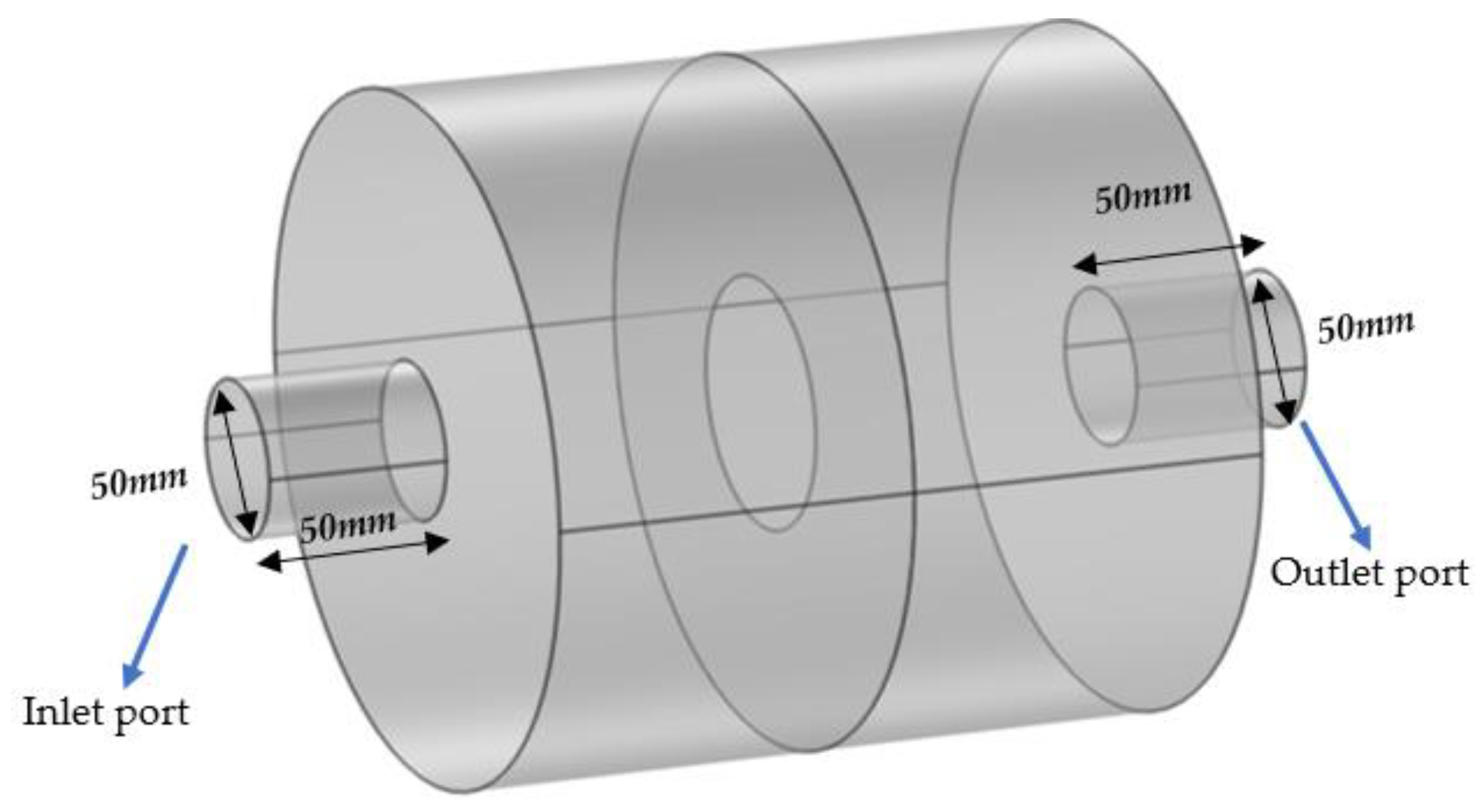
The dimension of the input and output tubes of the muffler, including length and diameters, are constant during the simulation of different parameters; see Figure 1.

A pressure acoustic model in the frequency domain is defined in COMSOL to simulate transmission loss in the muffler. The model specifications are as follows:

• All the volume is considered as pressure domain (use a single variable pressure acoustic for that);
• The outside and internal walls are sound hard boundary conditions (normal velocity is zero);
• Inlet port condition includes the combinational of an incoming and outgoing plane wave;
• Outlet port condition includes outgoing plane waves.

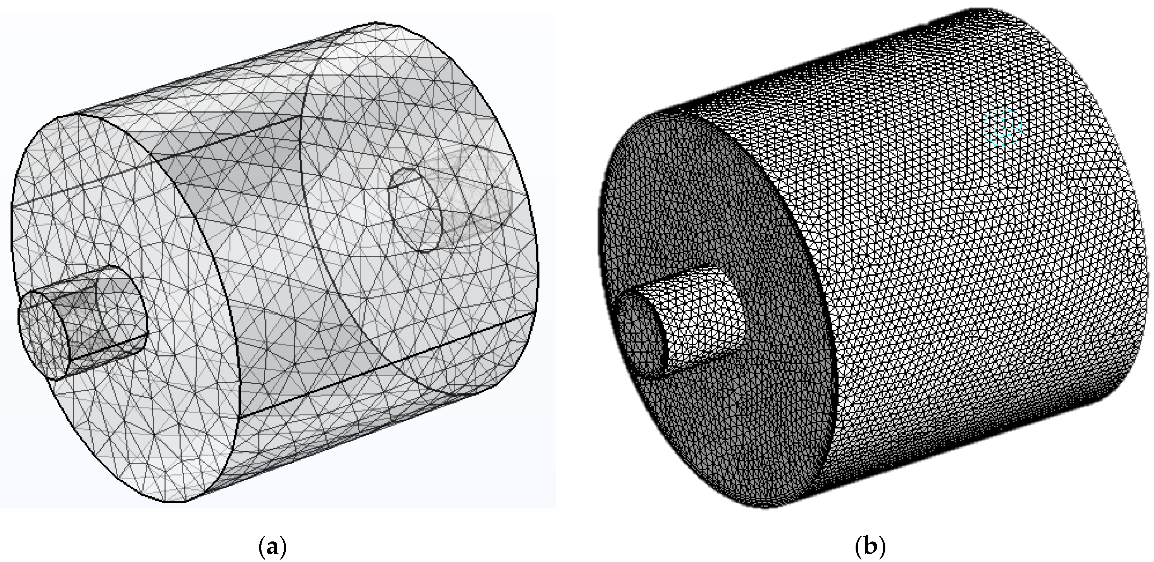
The model applies a free tetrahedral mesh element with a maximum element size equal to the speed of sound divided by five times the considered highest frequency [44]. The mesh of the muffler in acoustic simulation is shown in Figure 2a.

A modified Helmholtz equation for the acoustic pressure p is applied to simulate the acoustic behavior of the muffler [17].

$$\nabla ·\left(-\frac{\nabla p}{\rho }\right)-\frac{{\omega }^{2}p}{c^2\rho }=0$$

(3)

where

$\rho$ is the density,

$\omega$ is the angular frequency,

$c$ is the speed of sound.

3.1.2. CFD Simulation Model

The boundary conditions of the CFD model in Fluent software are assumed as follows:

• Mass-flow boundary condition is applied at the inlet;
• Pressure-outlet boundary condition is applied at the outlet;
• The wall function for exterior and interior surfaces is considered.

The pressure-based solver with steady time and the pseudo transient option is used in ANSYS Fluent. Unstructured tetrahedral elements are applied in simulation because of the complexity of geometry. ANSYS meshing was used to mesh geometry with linear order elements. The outer surfaces of inlet and outlet tubes and cylindrical chamber consist of 5 boundary layers. The maximum element size of the mesh is 3–5 mm. In Figure 2b, the CFD simulation mesh is shown.

In this study, the turbulent $k-\epsilon$ method for turbulence modeling is utilized in ANSYS Fluent. Two variables, $k$ and $\epsilon$, which stand for the kinetic energy and dissipation rate, respectively, are presented in the turbulent flow field. The turbulent viscosity is derived from the below equation [45]:

$${\mu }_t=C_{\mu }\rho \frac{k^2}{\epsilon }$$

(4)

where

${\mu }_t$ is the turbulent viscosity,

$C_{\mu }$ is the experimental coefficient.

The following quasi-experimental equations are solved by ANSYS Fluent to find the values of $k$ and $\epsilon$ [45]:

$$\begin{gathered} \mathsf{\rho }\frac{\partial \mathrm{k}}{\partial \mathrm{t}}+\mathsf{\rho }{u}_j{k}_{,j}={\left(\mu +\frac{{\mu }_t}{{\sigma }_k}{k}_{,j}\right)}_{,j}+G+B-\rho \epsilon ; \\ \mathsf{\rho }\frac{\partial \epsilon }{\partial \mathrm{t}}+\mathsf{\rho }{u}_j{\epsilon }_{,j}={\left(\mu +\frac{{\mu }_i}{{\sigma }_{\epsilon }}{\epsilon }_{,j}\right)}_{,j}+C_1\frac{\epsilon }{k}G+C_1\left(1-C_3\right)\frac{\epsilon }{k}B-C_2\mathsf{\rho }\frac{{\epsilon }^2}{k} \end{gathered}$$

(5)

where

$C_1, C_2$, and $C_3$ are experimental coefficients,

${\sigma }_{\epsilon }$ is turbulent Schmidt number,

${\sigma }_k$ is turbulent Prandtl number,

$G$ is the amount of turbulent kinetic energy produced when the mean flow interacts with the turbulent flow field,

$B$ stands for the generation of buoyancy loss.

$C_1\frac{\epsilon }{k}G$ and $C_2\mathsf{\rho }\frac{{\epsilon }^2}{k}$ describe the processes of shear generation and viscous dissolution, respectively, and $C_1\left(1-C_3\right)\frac{\epsilon }{k}B$ shows buoyancy effects.

The constants $C_1$, $C_2$, $C_{\mu }$, ${\sigma }_k$, and ${\sigma }_{\epsilon }$ have the following values [46]:

$C_1=1.44$, $C_2=1.92$, $C_{\mu }=0.09$, ${\sigma }_k=1.0$ and ${\sigma }_{\epsilon }=1.3$.

The results of these simulations are used for analyzing the muffler’s performance in each step of the design.

3.2. Objective Functions

The evaluation of design parameters can be an important process for identifying the factors that need to be controlled for high-performance mufflers. The objective function can be used to accomplish that. An objective function is a mathematical formula represented by $f\left(x\right)$, where $x$ is the set of design parameters and is used to optimize or evaluate a system or process [26]. These provide consistent and accurate measurements of acoustic performance, as well as a quantitative comparison of the simulation results.

In the context of muffler design, $f\left(x\right)$ is a measure of the acoustical performance of the muffler and $x$ is the set of design parameters that define the muffler geometry. The following objective function formula is selected to compare transmission loss curves for ith frequency interval in noise reduction [47].

$$f_i\left(x\right)=\overline{TL}\left({∆f}_i\right)=\frac{1}{f_{\mathrm{i}}-f_{\mathrm{i}-1}}{\int }_{f_{\mathrm{i}-1}}^{f_{\mathrm{i}}}TL\left(f\right)df$$

(6)

where

$f$ is a frequency variable.

$f_i$ is the end of ith frequency interval

$f_{i-1}$ is the beginning of ith frequency interval

Usually, the first few harmonics of the engine firing frequency (EFR) constitute the effective frequency range of interest. It means the dominant contribution of the noise is in that frequency range [36]. If measured sound data from the engine is available, this desired region can be specified more precisely. Using Equation (4), where Engine rpm is 9000 for the KTM 390 4-stroke engine, the calculated EFR equals 75 Hz. Accordingly, the first four harmonics of the EFR are considered for the desired region, including frequencies 75, 150, 275, and 350 Hz.

$$EFR=n\times \frac{Engine rpm}{120}$$

(7)

where

$EFR$ is engine firing frequency,

$n$ is a factor equal to 1 for a four-stroke engine (equal to 2 for a 2-stroke).

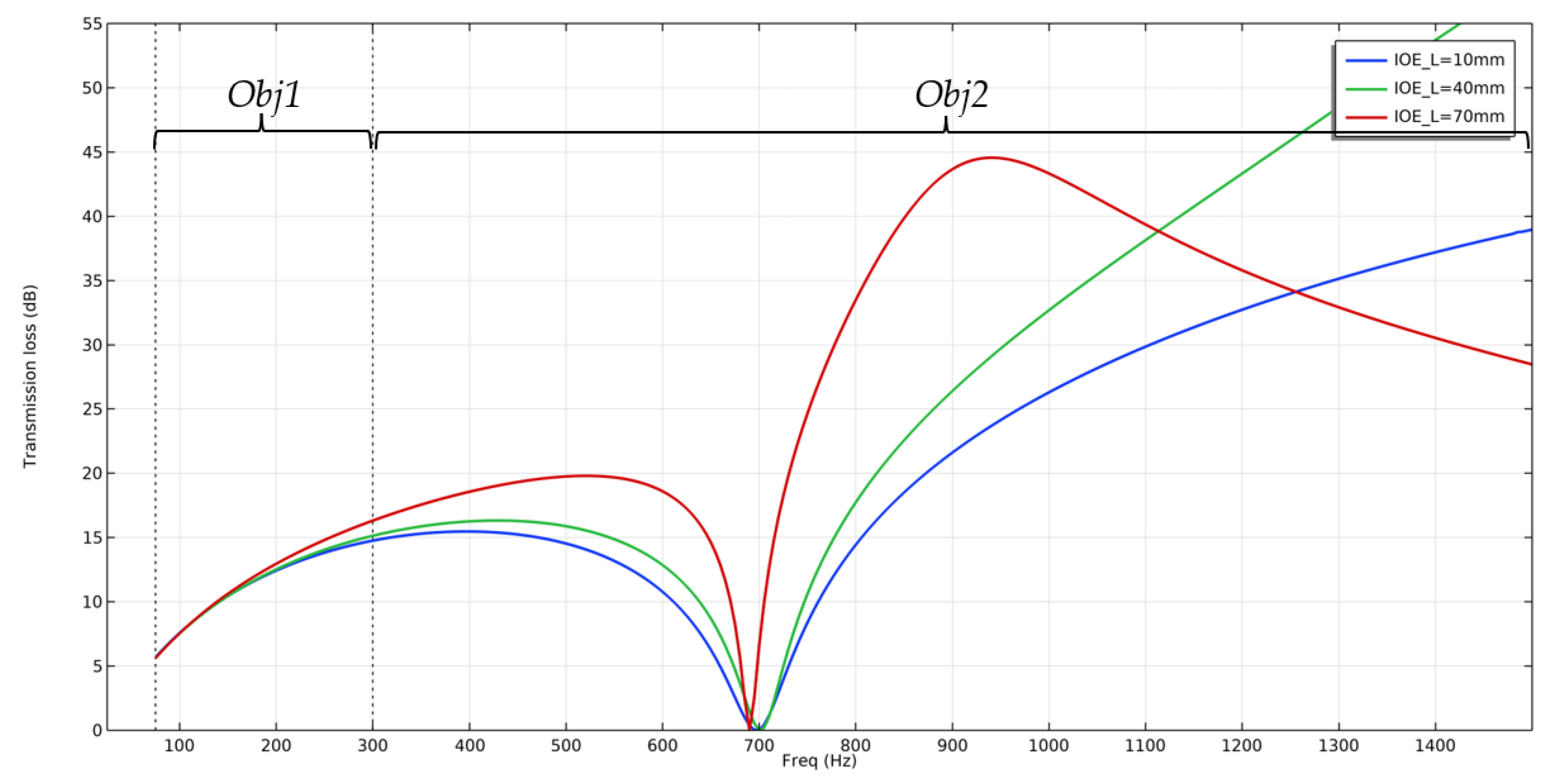
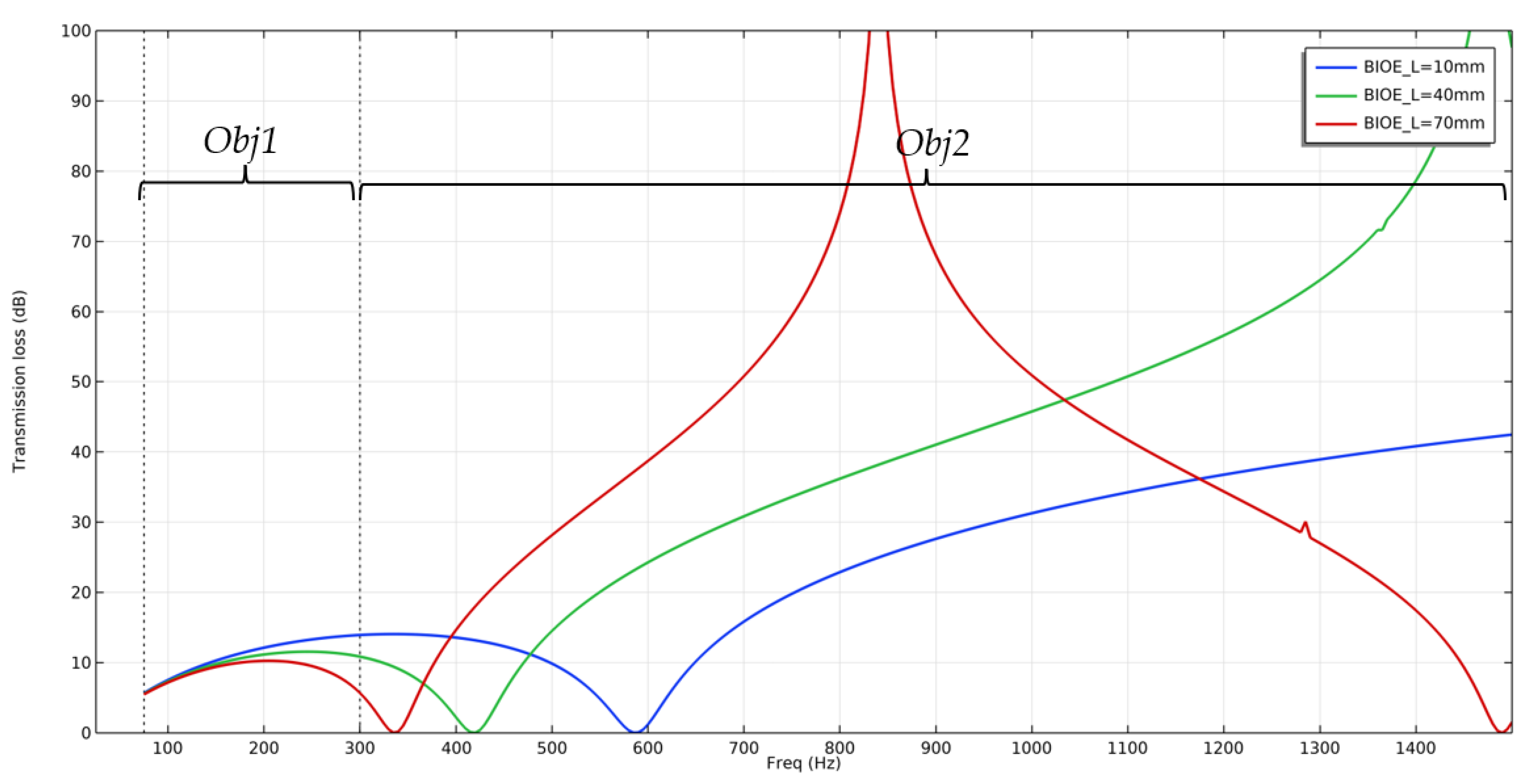
According to Equation (3), objective functions obj1 and obj2 are defined for frequency ranges of 75 to 300 Hz and greater than 300 Hz, respectively (see Equations (5) and (6)). The objective function obj1 is defined to contain the desired frequency region. For comparing different mufflers, these objective functions are evaluated in sequence. It means that first, the value of the obj1 should be acceptable so that the obj2 value can be used for comparison. Backpressure must also be specified as a constraint.

$$\mathit{obj}1=f_1\left(x\right)=\frac{1}{300-75}{\int }_{75}^{300}TL\left(f\right)df$$

(8)

$$\mathit{obj}2=f_2\left(x\right)=\frac{1}{1500-300}{\int }_{300}^{1500}TL\left(f\right)df$$

(9)

Furthermore, defining and evaluating these two objective functions in this order has a practical advantage. When the obj1s have an insignificant difference, the obj2 is useful for comparing the mufflers’ performance. In such instances, comparing obj2 provides an option for muffler performance evaluation.

3.3. Muffler Initial Length

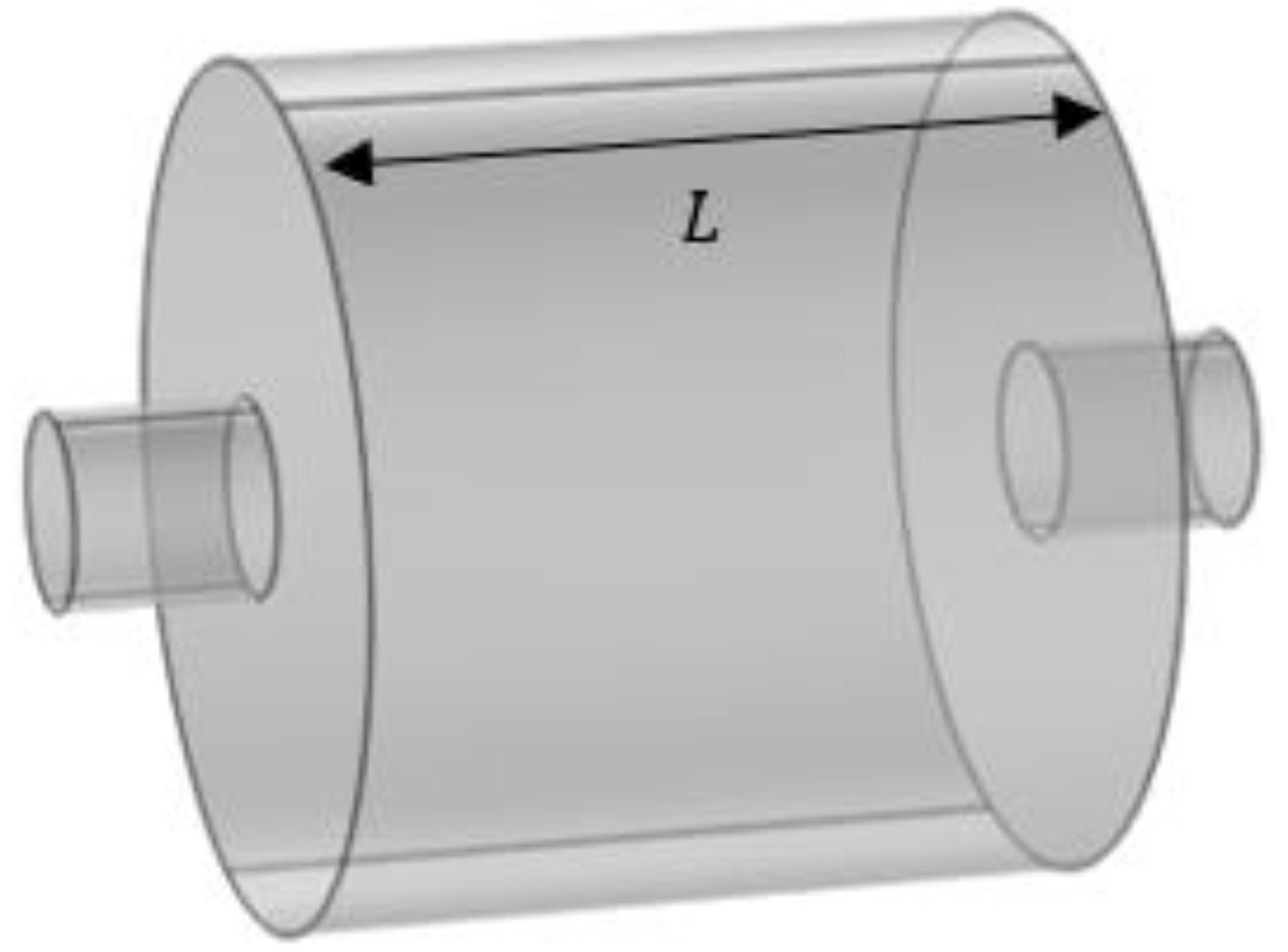
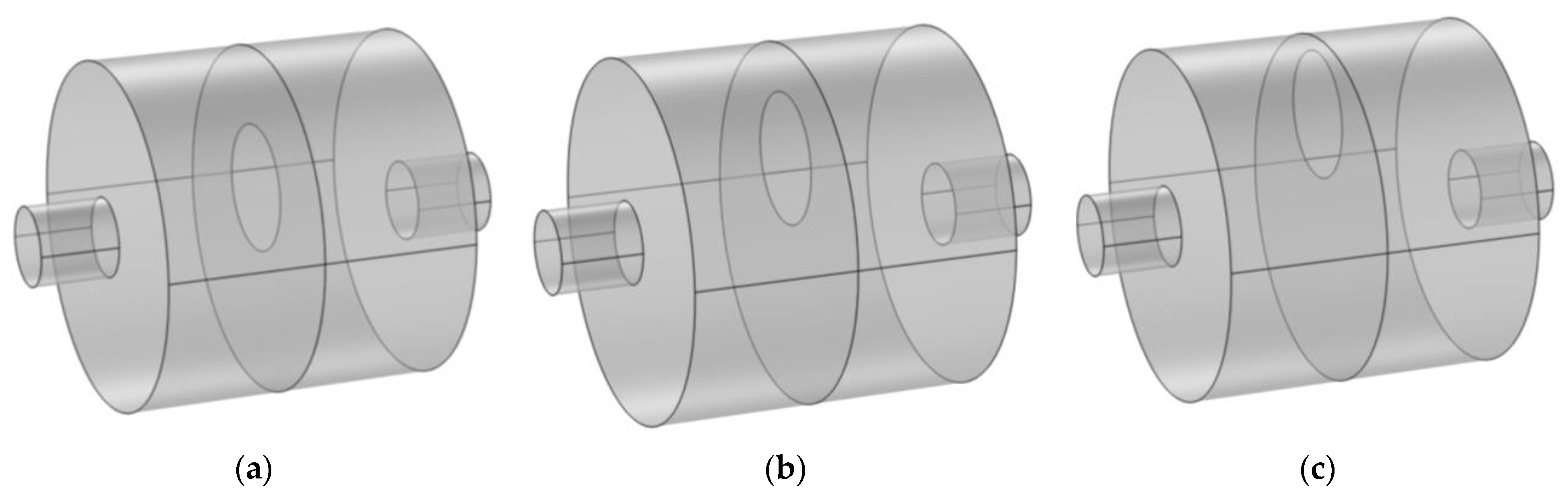
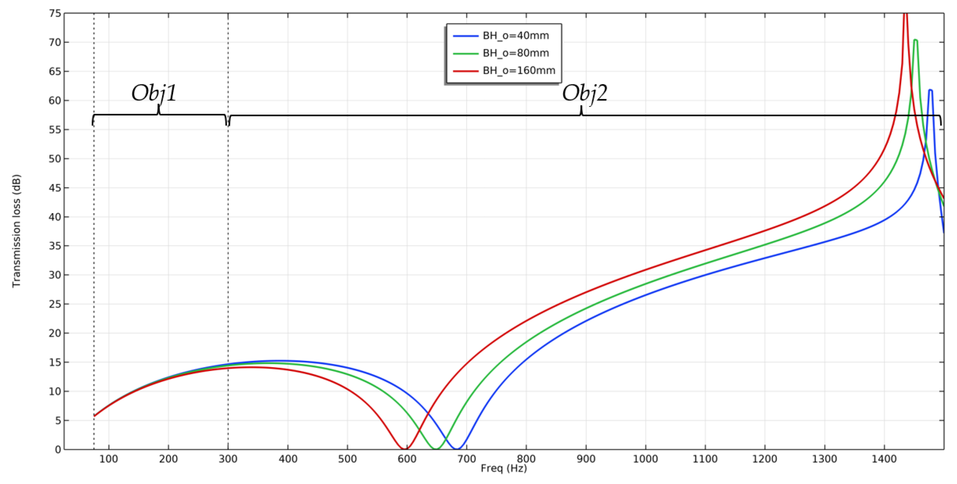
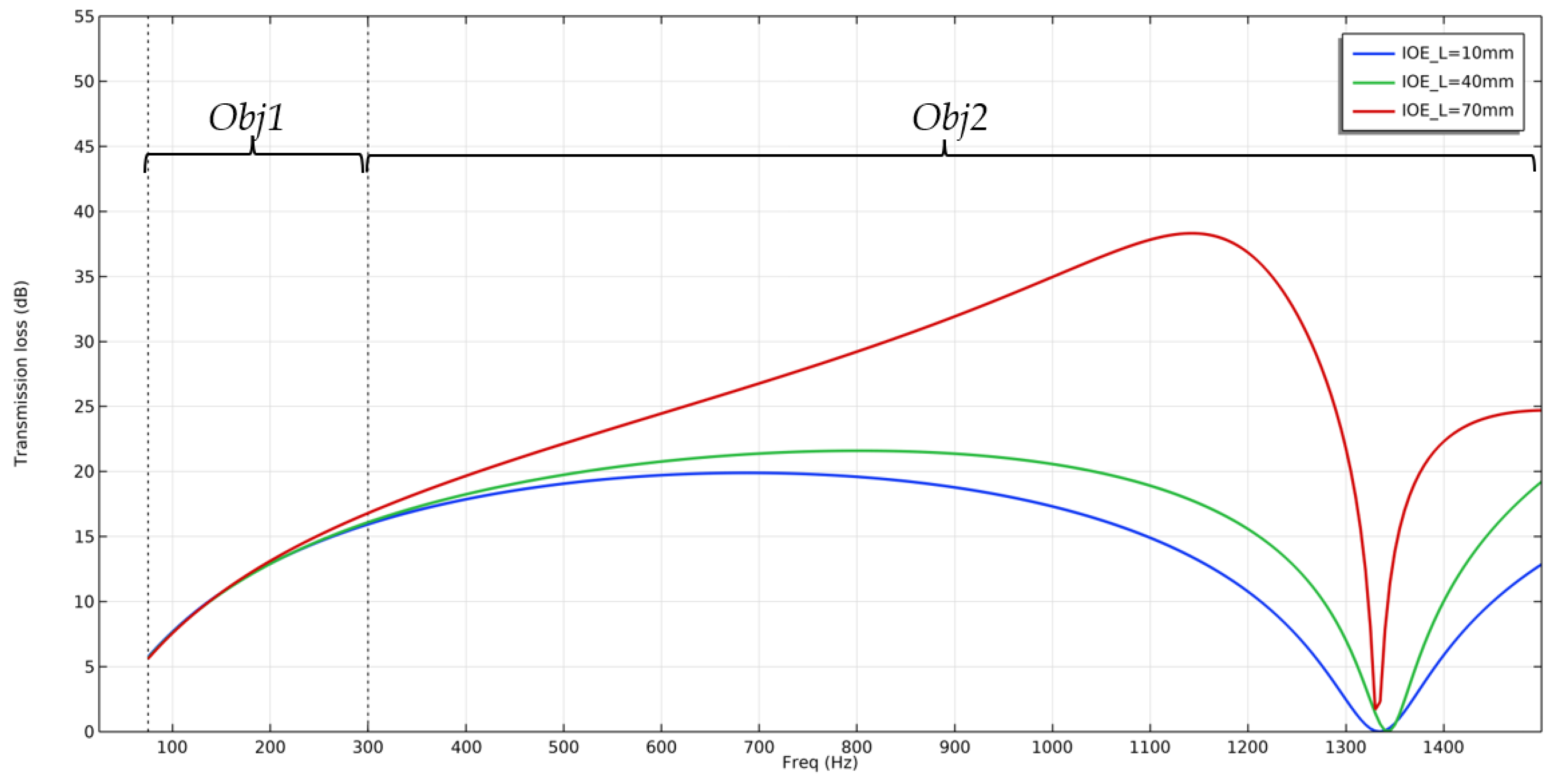
The overall dimensions of the muffler are determined by considering the volume limitation. The muffler’s volume is constant and the overall geometry is cylindrical. The length variable, shown in Figure 3, is selected by analyzing the variation of the transmission loss curve due to the length variable’s effect on the transmission loss in the specified frequency range. It is observed by increasing length values that obj1 and obj2 will decrease. 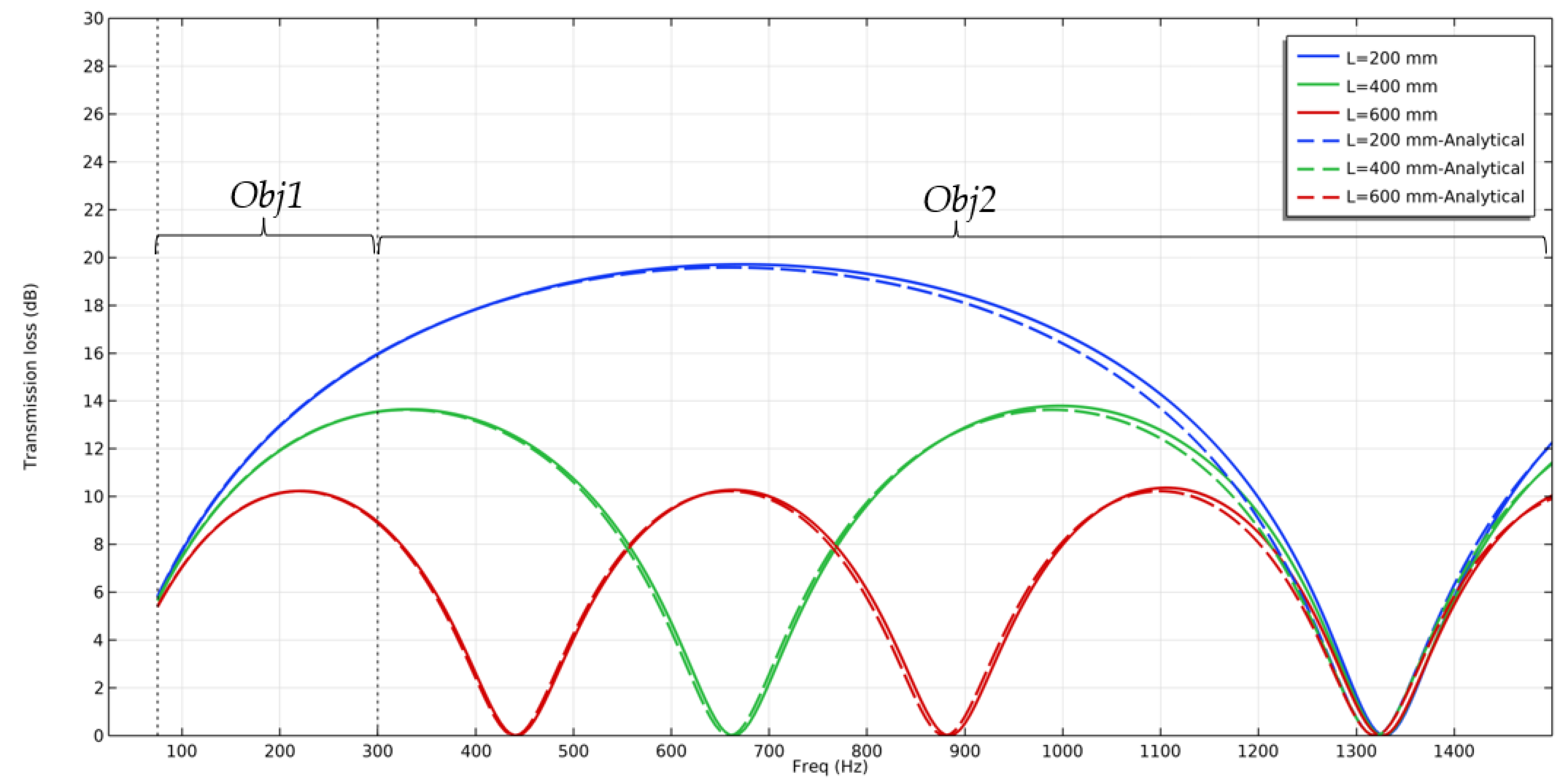Greater values of length cause an increase in obj1 and obj2. Zero point of transmission loss maintains constant around frequency 1320 Hz; see Figure 4.

The analytical Equation (7) represents TL for a simple expansion chamber with length $L$ [48]. The validation of results is shown in Figure 4, where there is a strong adaption between simulated results and analytical values for TL.

$$\mathrm{T}\mathrm{L}=10\mathrm{L}\mathrm{o}\mathrm{g}\left(1+\frac{m-1/m}{2}\sin kL\right)$$

(10)

where

$m$ is the effective area ratio equal to square of diameter ratio,

$k$ is the wave number,

$L$ is chamber’s length.

In order to evaluate how the muffler performance factors (including obj1, obj2, and backpressure) are affected by the corresponding parameter (within a specified range), we define criteria to measure the relative distance from the maximum value in percentage for each performance factor. It is called the percentage deviation of maximum (PDM) and its formula is as follows:

$$PDM\left(\%\right)=\frac{E_{i-max}-E_{i-min}}{E_{i-max}}\times 100, i=1, 2, 3$$

(11)

where

$i=1$ refers to obj1, and $E_{1-max}$ and $E_{1-min}$ are maximum and minimum values of obj1 for various values of the considered parameter,

$i=2$ refers to obj2, and $E_{2-max}$ and $E_{2-min}$ are maximum and minimum values of obj2 for various values of the considered parameter, and

$i=3$ refers to backpressure, and $E_{3-max}$ and $E_{3-min}$ are maximum and minimum values of backpressure for various values of the considered parameter.

The total dimension quantities resulting from the simulation with the help of computational measurement are shown in

Table 2. Simulation results of length $L$.

Parameter “L”	Obj1	Obj2	Backpressure (kpa)
200 mm	11.9	14.7	3.13
400 mm	10.9	9	8.18
600 mm	9.1	6.2	10.07

. Backpressure, obj1, and obj2 change (PDM %) by 68.9%, 23.5%, and 57.8%, respectively. Therefore, the more suitable length in terms of obj1, obj2, and backpressure was 200 mm where the highest obj1 and obj2 and lowest backpressure values were obtained.

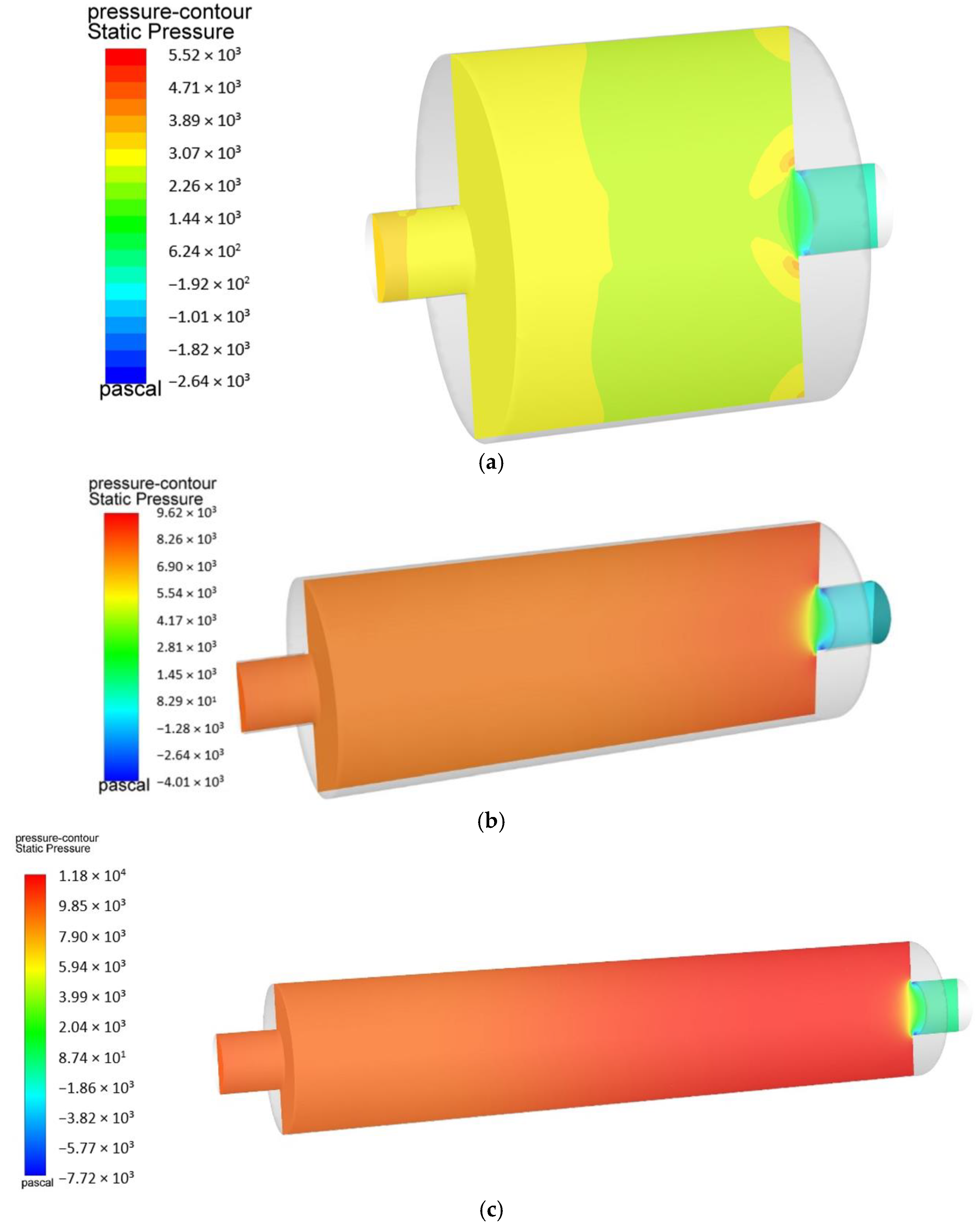
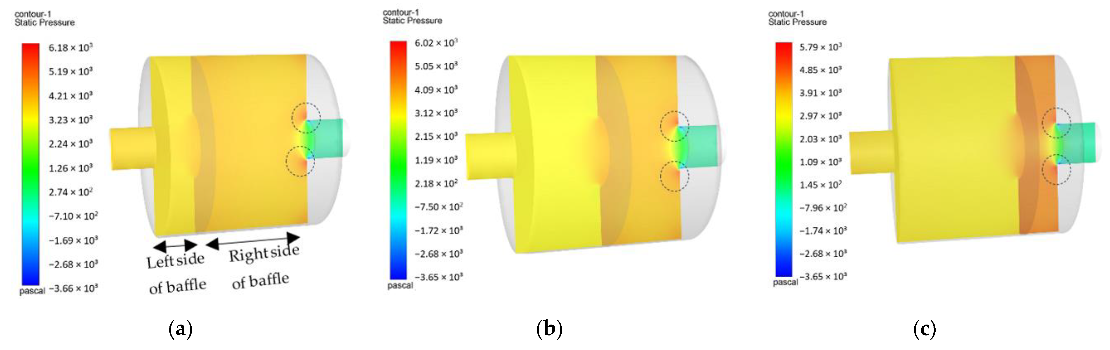
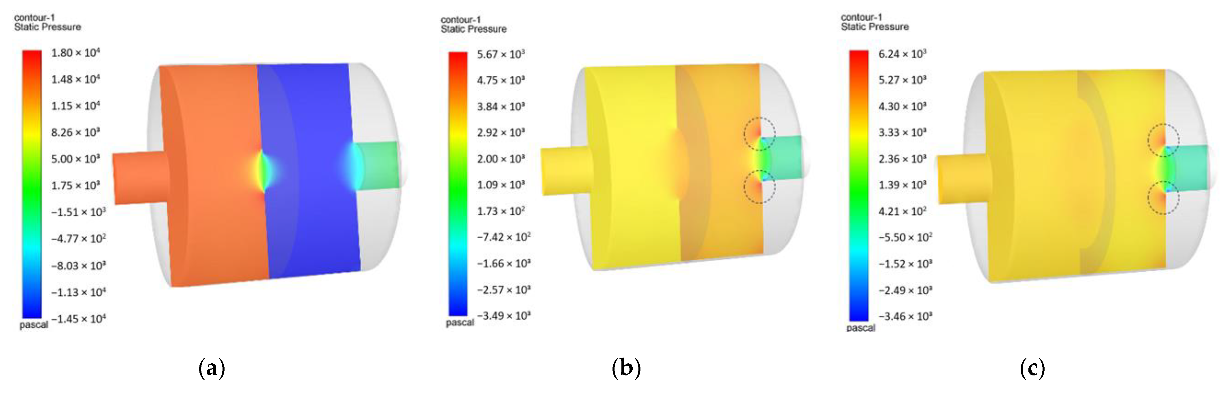
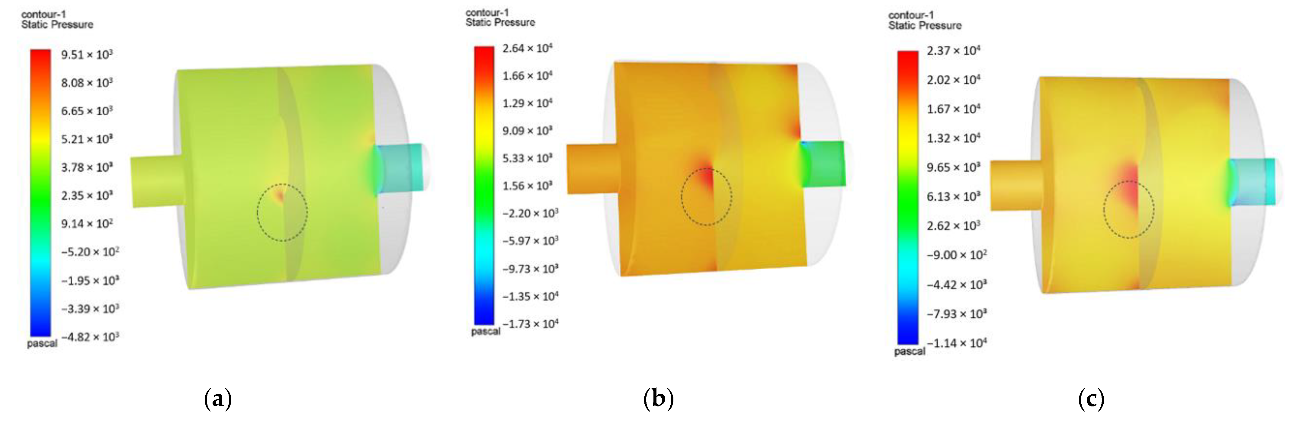
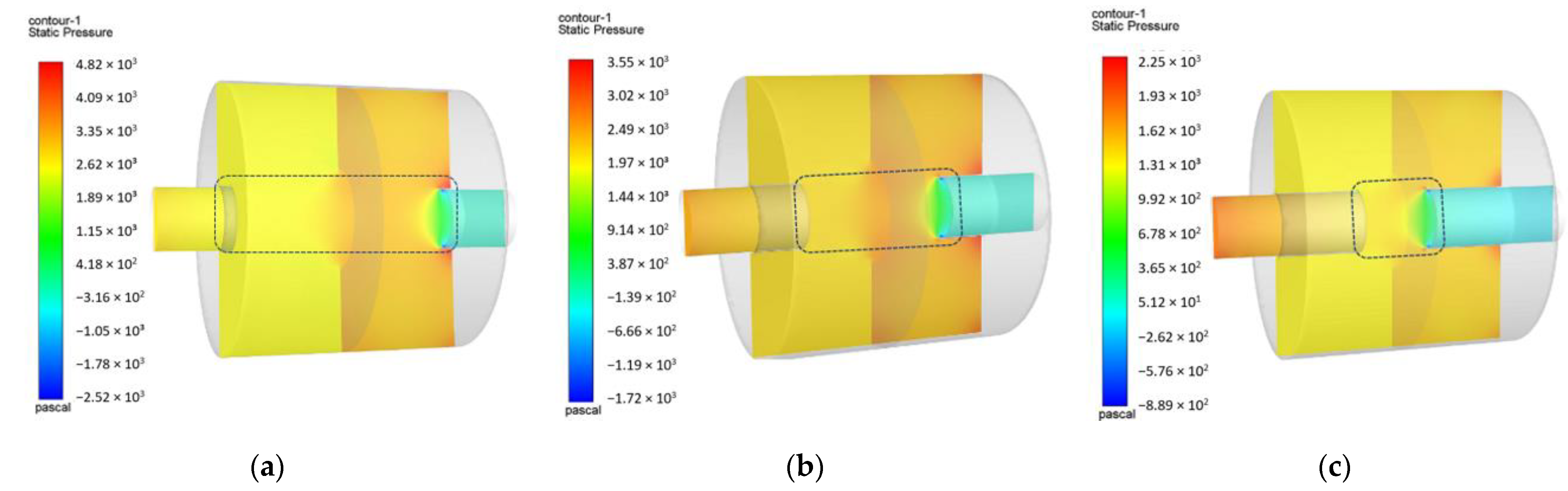
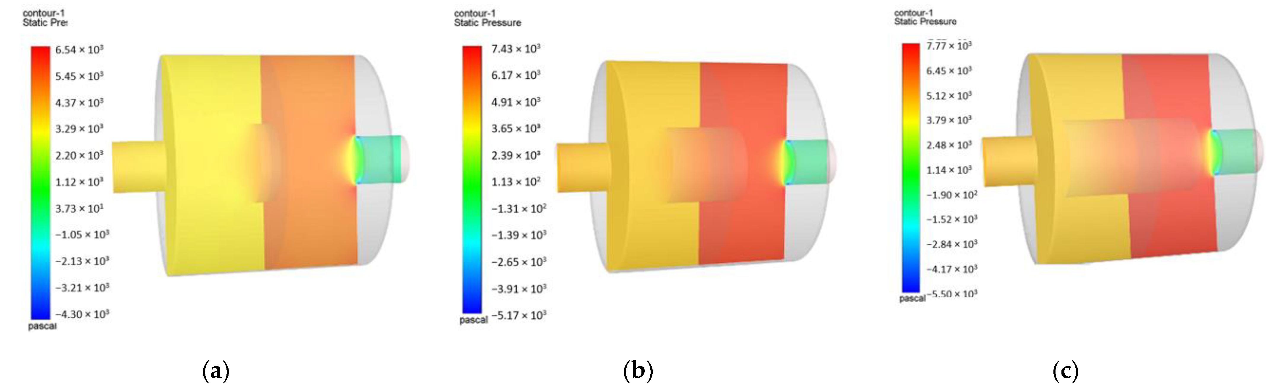
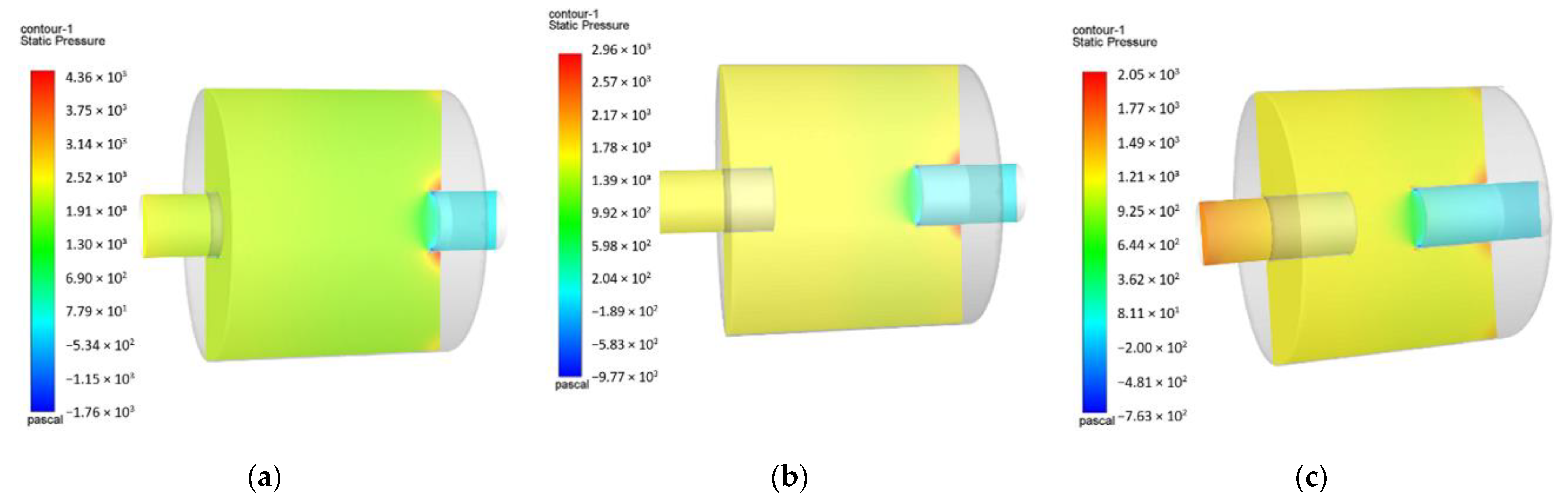
The backpressure column in Table 2 is extracted from CFD simulations that are shown in Figure 5. It is seen that the maximum pressure which is inside the chamber and vicinity of the outlet tube can be more than the backpressure. The maximum inside pressure, and backpressure increase with decrement in the chamber’s diameter (equivalent to the increase in the length with constant volume).

In this step, a 200 mm length was selected and will be used in the next steps of simulation. The initial dimension according to this selection is considered for the rest of the design process of the muffler.

3.4. Methodology of Design and Analysis of a Muffler

As mentioned above, there are many factors which are affecting on of the muffler’s performance. Therefore, a method for organizing those factors in a proper sequence leading to designing a muffler with good performance is presented. This process starts with primary geometry and then other features are added to complete the designing process with more details. Each feature includes some parameters named “subfeatures” which affect the overall performance of the muffler. In each feature, some analyses are performed on the subfeatures in order to select the best. Then, we proceed to the next feature.

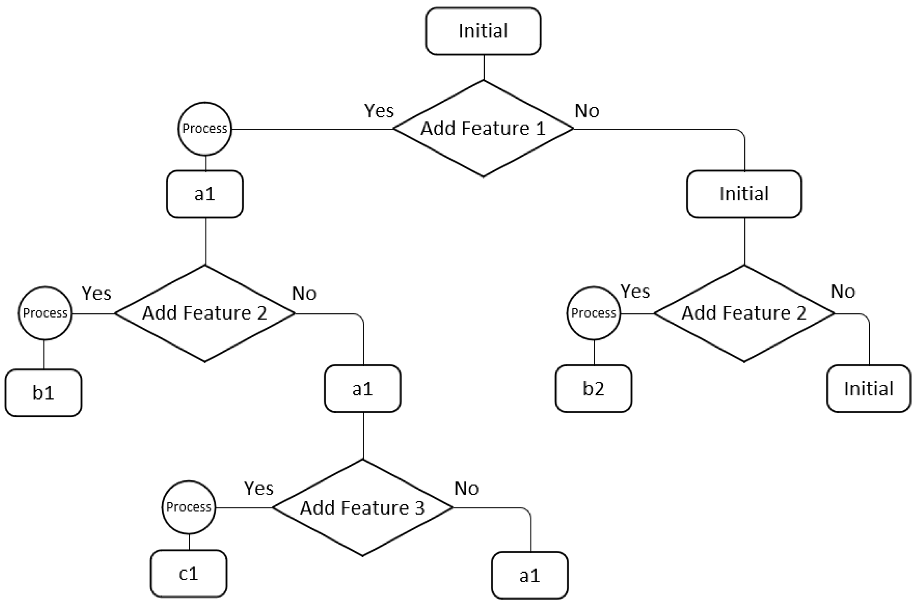
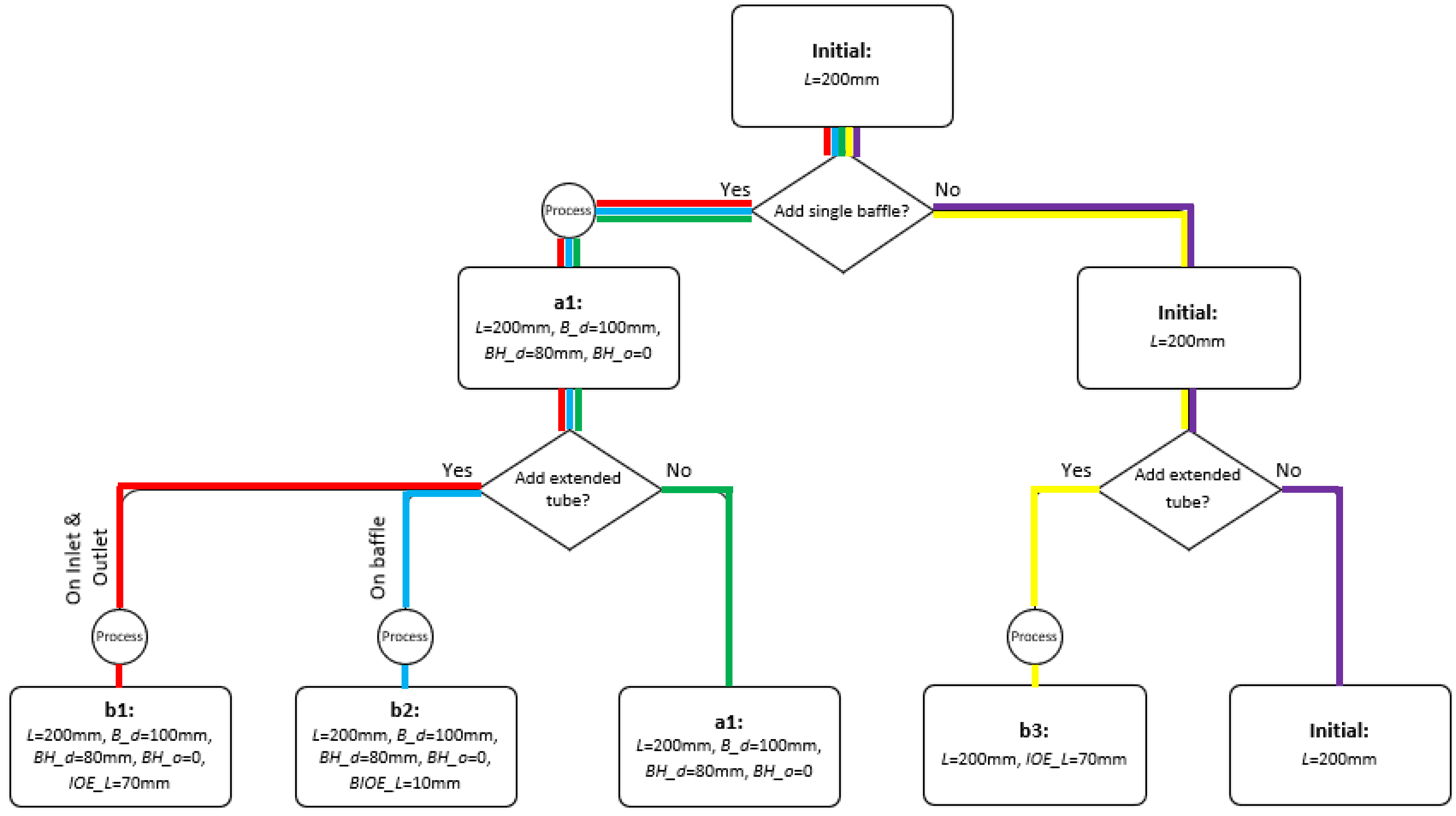
A tree diagram, depicted in Figure 6, was used to show the designing process in an understandable way. In this figure, each rectangle represents a different state (with its specified subfeatures values) of the muffler (each state may have specific geometry, dimensions, or parameters), and each branch (in a diamond shape) indicates a decision on whether a feature should be added to the upper state of the muffler (the state before the diamond decision) or not. Then, a process on each feature to specify the best sub-feature (equivalent to the process of choosing a value for a related parameter) is conducted to optimize the muffler performances. Circles in the tree diagram represent this processing unit. The last step is considering all selected states which are placed in the tree leaves, including b1, c1, a1, b2, and initials in Figure 6, and identifying the best state based on the performance evaluation of the results.

According to the organized process in Figure 6, we need to find the simulation results for each change of features and subfeatures, and then by analyzing and comparing the simulation results, a desirable feature and subfeature are considered and the corresponding muffler states are specified. The process continues until all the mentioned features of the muffler will be considered. The simulation results of each step are discussed as follows, and at the end, according to these obtained results and analysis, this figure will be transformed and detailed. 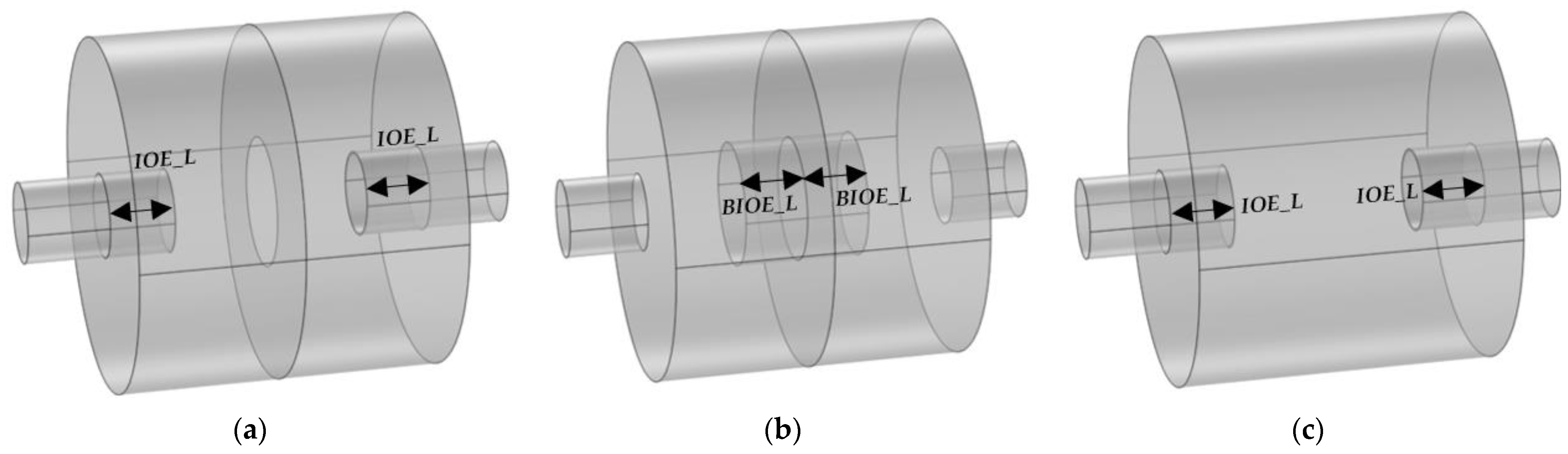The initial state in this study is determined by optimizing the length of the muffler, which was specified in Section 3.3. The main features are baffle and extended tube length with their subfeatures, which will be analyzed and specified in the next part.

4. Results and Analysis

The performance results of the designed muffler for each feature and subfeature are analyzed and compared based on the methodology analysis mentioned in Figure 6. Therefore, the simulation results of each feature and subfeature are presented and discussed in this section. Accordingly, the best amount of those features is selected based on comparing the backpressure, obj1, and obj2 results, and finally, this process will be summarized in a tree diagram similar to Figure 6 while it is carried out for this case study.

4.1. First Feature: Baffle

Various parameters of baffles, including a cut of ratio, number of holes, and distance, effectively reduce the muffler’s sound and pressure drop [49]. This section evaluates the baffle’s presence, its appropriate location, and fluid passage in the muffler. A detailed investigation of the baffle parameters on sound reduction is outside the scope of this article. The baffle location, diameter, and hole location parameters are investigated as a case study, illustrated in Figure 7.

4.1.1. First Subfeature of Baffle: Baffle Distance

Figure 7a shows the parameter B_d, which represents the distance of the baffle from the entrance, and Figure 8 represents the considered various amounts of this distance.

Table 3. Simulation results of baffle distance, $B\_d$.

Parameter “B_d”	Obj1	Obj2	Backpressure (kpa)
50 mm	11.6	20.8	3.75
100 mm	11.4	21.7	3.32
150 mm	11.6	20.8	3.47

shows the simulation results for various baffle distance values where the hole diameter of the baffle is 80 mm. Changing the value from 50 to 150 mm can affect obj1 and obj2 by 1.7% and 4.1%, respectively, and backpressure by 11.5% (PDM % according to Equation (11)). Figure 9 depicts the transmission loss curve as the parameter B_d changes. The minimum point of the graph decreases from 790 Hz to around 700 Hz as the parameter value increases from 50 to 100 mm. The graph returns to first place, increasing from 100 to 150 mm.

Furthermore, the backpressure results based on CFD simulations are shown in Figure 10. Accordingly, the pressure on the right side of the baffle is greater than that on the left side of the baffle. The pressure distribution inside the muffler shows areas with the highest pressure occurring around the outlet. In Figure 10, it can be seen that the backpressure is not significantly changed from (a) to (c) by increasing the B_d from 50 mm to 150 mm. Based on the performance results in Table 3, obj1 has insignificant change, and obj2 and the backpressure slightly improved; therefore, a value of 100 mm is chosen for baffle distance (B_d) in this step.

4.1.2. Second Subfeature of Baffle: Baffle Hole Diameter

Figure 7b illustrates the parameter baffle hole diameter (BH_d) and its various amounts considered for this study are depicted in Figure 11. The transmission loss curve is drawn with the change of the BH_d parameter; see Figure 12. By increasing the values from 40 to 160 mm, the graph’s minimum point increased from 430 Hz to around 1190 Hz. The transmission loss curve converges to the muffler without a baffle, as shown in Figure 3 (with a length of 200 mm).

Table 4. Simulation results of baffle hole diameter ($BH\_d$).

Parameter “$\mathit{B}\mathit{H}\_\mathit{d}$”	Obj1	Obj2	Backpressure (kpa)
40 mm	10.1	30.8	15.42
80 mm	11.4	21.7	3.32
160 mm	11.9	14.6	3.98

shows the values of the objective functions. Obj1 and Obj2 values have changed by 15.1% and 52.6%, respectively, and backpressure has changed by 78.5% (PDM % in Equation (11)). The backpressure significantly increases in the diameter of 40 mm; therefore, it is inappropriate and far from the requirement of 3.3 kpa. A diameter of 80 mm, compared to 160 mm, has a little lower value of obj1, while obj2 has a significantly higher value. In addition, its backpressure is low; therefore, it is selected.

Moreover, according to the results of CFD simulations as illustrated in Figure 13a, the right side of the baffle shows significant negative pressure (approximately 14 kpa), and the muffler has a very high value of backpressure (15.42 kpa). Increasing the diameter from Figure 13a–c lead to a decrease in the pressure difference between both sides of the baffle, and consequently, the highest pressure areas around the outlet are being appeared from (a) to (c). In addition, the negative pressure area in Figure 13a is eliminated in (b) and (c) by increasing the BH_d from 40 mm to 80 mm and 160 mm, respectively. In consequence, (b) and (c) in Figure 13 are better choices, and considering the Table 4 analysis, the baffle’s hole diameter ($BH\_d$) equal to 80 mm is selected and will be used in the following steps of simulation.

4.1.3. Third Subfeature of Baffle: Baffle Hole Offset

The parameter baffle hole offset (BH_o) is shown in Figure 7c and its different values for analysis are plotted in Figure 14. With the increase in BH_o, the minimum point of the graph decreases from 690 to about 600 Hz; see Figure 15.

According to

Table 5. Simulation results of baffle hole offset ($BH\_o$).

Parameter “$\mathit{B}\mathit{H}\_\mathit{o}$”	Obj1	Obj2	Backpressure (kpa)
20 mm	11.4	23.1	4.83
40 mm	11.3	25.0	13.57
60 mm	11.1	26.8	16.85

, obj1 and obj2 changed by 2.6% and 13.8%, respectively, while backpressure changed by 71.3% (PDM % in Equation (11)). Due to this increase in this parameter, the backpressure increased significantly. When the 20 mm value of BH_o in Table 5 is compared to the corresponding values of the selected muffler in Table 4 (BH_d equals 80 mm), obj2 improves slightly (6%) but backpressure increases significantly (31.3%). Therefore, the zero value of BH_o is chosen.

In addition, the results of CFD simulations illustrated in Figure 16 show that increasing BH_o from (a) to (c) results in significantly higher values of the backpressure, indicating more flow resistance. As a result, deviation of the flow from the straight path can have a considerable degradation effect on aerodynamic performance. According to the pressure distribution inside the muffler in Figure 16, areas with the highest pressure occur in the closest points around the baffle hole.

The simulation results in Figure 15 and Figure 16 and Table 5 show that the zero value of baffle hole offset is more effective. Thus, this subfeature is not considered for designing this muffler.

4.2. Second Feature: Extended Tube Length

The effect of extension length can be applied to the baffle’s hole, and the inlet and outlet pipes separately. In addition, this effect should be analyzed on the muffler with and without the baffle. These various states of the applied extension tube length on the muffler are illustrated in Figure 17.

4.2.1. First Subfeature of Extended Tube: Inlet and Outlet Extension Length with Baffle

The inlet and outlet extension length parameter (IOE_L) is represented in Figure 17a for the muffler with the baffle. By increasing the length of the inlet and outlet pipes (equally), the minimum point of the graph remains at around 700 Hz, but both the right and left sides of this point have increased, see Figure 18.

According to

Table 6. Simulation results of inlet and outlet extension length ($IOE\_L$) for the baffled muffler.

Parameter “$\mathit{I}\mathit{O}\mathit{E}\_\mathit{L}$”	Obj1	Obj2	Backpressure (kpa)
10 mm	11.4	22.3	2.85
40 mm	11.5	28.8	2.54
70 mm	12.0	29.2	1.84

, obj1 and obj2 have increased by 5% and 23.6%, respectively. In addition, backpressure has decreased by 35.4% (PDM % in Equation (11)). In other words, all three factors have improved. Therefore, the value of 70 mm is desirable.

Additionally, according to CFD simulations in Figure 19, the maximum amount of pressure distribution takes place around the intersection of the right wall and outlet extended pipe. Increasing the extension length brings about reducing the backpressure since the flow path has been guided more straightly. As a result, in this step, the value of the inlet and outlet extension length for the muffler with a baffle equal to 70 mm is selected.

4.2.2. Second Subfeature of Extended Tube: Baffle Inlet and Outlet Extension Length

The parameter BIOE_L shows the extended length of the baffle’s hole; see Figure 17b. The minimum point of the transmission loss curve is reduced from 600 Hz to 340 Hz by increasing the BIOE_L parameter; see Figure 20.

Based on the simulation results in

Table 7. Simulation results of inlet and outlet extension length ($BIOE\_L$) of the baffle’s hole.

Parameter “$\mathit{B}\mathit{I}\mathit{O}\mathit{E}\_\mathit{L}$”	Obj1	Obj2	Backpressure (kpa)
10 mm	11.1	25.2	4.17
40 mm	10.1	42.2	4.84
70 mm	8.8	38.1	5.06

, obj1 is reduced by 20.1%. Obj2 at first increases and then decreases in the range of 40.3% (PDM % in Equation (11)). The backpressure has also increased by 17.6%. Because of the priority of obj1 to obj2, the value of 10 mm is the best choice.

Additionally, as observed in the CFD simulations in Figure 21, an increase in the extension length of the baffle hole from (a) to (c) causes higher values of the backpressure and more pressure difference between the region’s right and left sides of the baffle. This simulation analysis shows that increasing the BIOE_L does not improve the muffler performance. Thus, in this step, baffle inlet and outlet extension length (BIOE_L) equal to 10 mm is chosen.

4.2.3. Third Subfeature of Extended Tube: Inlet and Outlet Extension Length without Baffle

By increasing the length of the inlet and outlet pipes in the muffler without a baffle (see Figure 17c), the minimum point of the transmission loss curve, which is evident in Figure 22, remains constant at around 1340 Hz. The transmission loss curve rises as a result of this increase, as shown in Figure 22.

According to

Table 8. Simulation results of inlet and outlet extension length ($IOE\_L$) in muffler without baffle.

Parameter “$\mathit{I}\mathit{O}\mathit{E}\_\mathit{L}$”	Obj1	Obj2	Backpressure (kpa)
10 mm	11.9	15.0	2.44
40 mm	11.9	17.6	1.95
70 mm	12.1	27.1	1.62

, increasing the IOE_L parameter from 10 to 70 mm enhances obj1 and obj2 by 1.6% and 44.6%, respectively, while decreasing backpressure by 33.6% (PDM % in Equation (11)). Since all three factors have improved for the parameter value 70 mm, this subfeature and its value were picked.

For more details, according to Figure 23, CFD simulations of IOE_L variations without baffle, the maximum amount of inside pressure happens around the intersection of the right wall and extended outlet tube. The increase in the extension length leads to a decrease in backpressure and maximum pressure. This can have the same reason for increasing IOE_L with baffle, as shown in Figure 19, where the flow path can be guided more straightly.

To compare these results with another study’s results, consider Middelberg et al. (2004) work relevant to our work in regard to the muffler shape and geometries. He compared three different configurations of mufflers, including a simple expansion chamber (similar to Figure 3), extended inlet/outlet pipes (similar to Figure 14c), and a baffle in the middle of the chamber (similar to Figure 8b), and concluded that extended inlet/outlet pipes muffler had significantly less backpressure than others [23]. Similarly, in our study, extended inlet/outlet pipes mufflers (see Figure 17c) have the lowest backpressure against two others (the backpressure column in Table 8 for extended inlet/outlet pipes mufflers has much lower values than Table 2 and Table 4 for simple expansion chamber and middle baffle mufflers).

4.3. Resulted Tree Diagram

Based on the simulation results above in this work, designing a muffler for the KTM90 engine, the tree diagram sample in Figure 6 is transformed into Figure 24.

In this regard, simulation results (Table 2) of the primary muffler (Figure 3) show that the total dimension with a length equal to 200 mm performs better than other lengths (initial state on Figure 24). The initial state without considering any other feature follows the purple color line highlighted in Figure 24. After that, a single baffle feature is added. Its subfeatures, including location, hole diameter, and the hole’s offset, are simulated in Section 4.1. As a result, the baffle location in the middle (B_d equals 100 mm) with BH_d equal to 80 mm and zero value of BH_o parameter, which has better performance in obj1, obj2, and backpressure, was selected (state a1 in Figure 24).

Following that, an extension tube feature is appended. Its related subfeature includes inside and outside extension length. State a1 without the extended tube is marked by green color in Figure 24. State b3 (highlighted in yellow color) is the muffler with the optimized length of the inlet and outlet extension tube without baffle. It is illustrated in Figure 17c, and Section 4.2.3 shows its corresponding simulation results. Adding an extension in the baffled muffler (add to state a1) can be done in two ways. First state where the extension tube is just on the baffle hole as shown in Figure 17b. The optimized length of the output extension tube in this state (analyzed and obtained in Section 4.2.2) is the muffler in state b2 (picked out in blue color) of the tree diagram (Figure 24). In the second state, the extension tube is only on the inside and outside tubes of the muffler; see Figure 17a. State b1 (highlighted in red color) in Figure 24 includes the details of the selected inlet and outlet extension length (in Section 4.2.1), in addition to the details of the selected baffle (state a1).

Finally, the performances of the leaves’ states in Figure 24 are compared as presented in

Table 9. Comparison of leaves in tree diagram.

State	Obj1	Obj2	Backpressure (kpa)
initial (Figure 3)	11.9	14.7	3.13
a1 (Figure 7b)	11.4	21.7	3.32
b1 (Figure 17a)	12.0	29.2	1.84
b2 (Figure 17b)	11.1	25.2	4.17
b3 (Figure 17c)	12.1	27.1	1.62

. Accordingly, states b1 and b3 bring about more efficient performance on obj1 and led to a much lower backpressure value than 3.3 kpa (allowable limit according to requirements in Section 2.3), while state b1 causes a higher value of obj2. Therefore, state b1 has the best performance and is the ultimate design chosen for the muffler.

4.4. Muffler Efficiency and Parameter Effectiveness

By defining muffler efficiency percentage as follows, the design process performance efficiency in terms of objective functions and backpressure is summed up:

$$efficiency \left(\%\right)=\frac{E_i-E_{i-ini}}{E_{i-ini}}\times 100, i=1, 2, 3$$

(12)

where

$i=1$ refers to obj1, and $E_1$ and $E_{1-ini}$ are values of obj1 for the design and initial state,

$i=2$ refers to obj2, and $E_2$ and $E_{2-ini}$ are values of obj2 for the design and initial state, and

$i=3$ refers to backpressure, and $E_3$ and $E_{3-ini}$ are values of backpressure for the design and initial state.

The performance efficiency of the different designed muffler states is compared in

Table 10. Comparison of improved performance criteria among different muffler states (bold percentages pointed out for improvement).

State	Obj1	Obj2	Backpressure (kpa)
initial	0	0	0
a1	−4.2%	+47.6%	+6.1%
b1 (selected)	+0.8%	+98.6%	−41.2%
b2	−6.7%	+71.4%	+33.2%
b3	+1.7%	+84.4%	−48.2%

. The plus sign for obj1 and obj2 shows improvement, while the minus sign for backpressure indicates enhancement. Therefore, the quantitative efficiency on obj1, obj2, and backpressure are improved by +0.8%, +98.6%, and −41.2%, respectively, in selected states.

The muffler design process can be more reliable by using the organized tree diagram method and less susceptible to miss-tracking different parameters’ effects on muffler performance. As a case, if state b1 missed and state b3 was selected (because of the higher value of obj1 and less backpressure against other remaining states), we have a degradation in performance efficiency of obj2 equal to 14.2%, respectively.

Evaluating the transmission loss trend with changing a parameter, gives us a comprehensive understanding of the parameter’s effect. PDM % (according to Equation (11)) of the muffler performance (obj1, obj2, and backpressure) for the selected parameters of the design is calculated (within the range of parameter values) and summarized in

Table 11. Comparison of PDM % of muffler performance for different parameters.

Parameter	PDM % of Obj1	PDM % of Obj2	PDM % of Backpressure
$L$ (Figure 3)	23.5%	57.8%	68.9%
$B\_d$ (Figure 7a)	1.7%	4.1%	11.5%
$BH\_d$ (Figure 7b)	15.1%	52.6%	78.5%
$BH\_o$ (Figure 7c)	2.6%	13.8%	71.3%
$IOE\_L$ (Figure 13a)	5%	23.6%	35.4%
$BIOE\_L$ (Figure 13b)	20.1%	40.3%	17.6%
$IOE\_L$ (Figure 13c)	1.6%	44.6%	33.6%

.

It is found that objective functions are highly dependent on L, BH_d, and $BIOE\_L$ and slightly dependent $B\_d$. Similarly, the backpressure is highly dependent on parameters $L$, $BH\_d,$ and $BH\_o$ and slightly dependent on $B\_d$.

5. Conclusions

A well-organized method for designing a muffler was proposed and acoustic and aerodynamic performances of the muffler in each step of designing were analyzed in COMSOL and ANSYS Fluent with suggested quantitative assessments obj1, obj2, and backpressure, and, accordingly, the suitable parameters were selected. This process has been performed for designing a muffler for the KTM390 engine as a case study. Considering obj1, obj2, and backpressure in an organized manner for evaluation and selection of suggested features and subfeatures led to a new method for designing a high-performance muffler design.

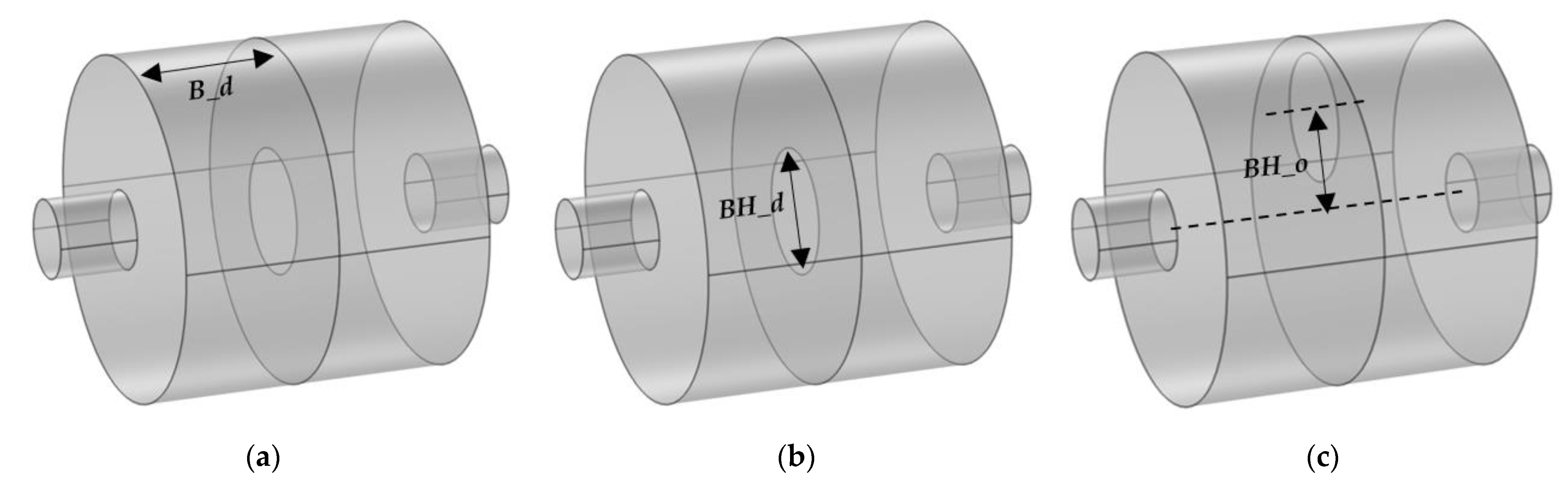
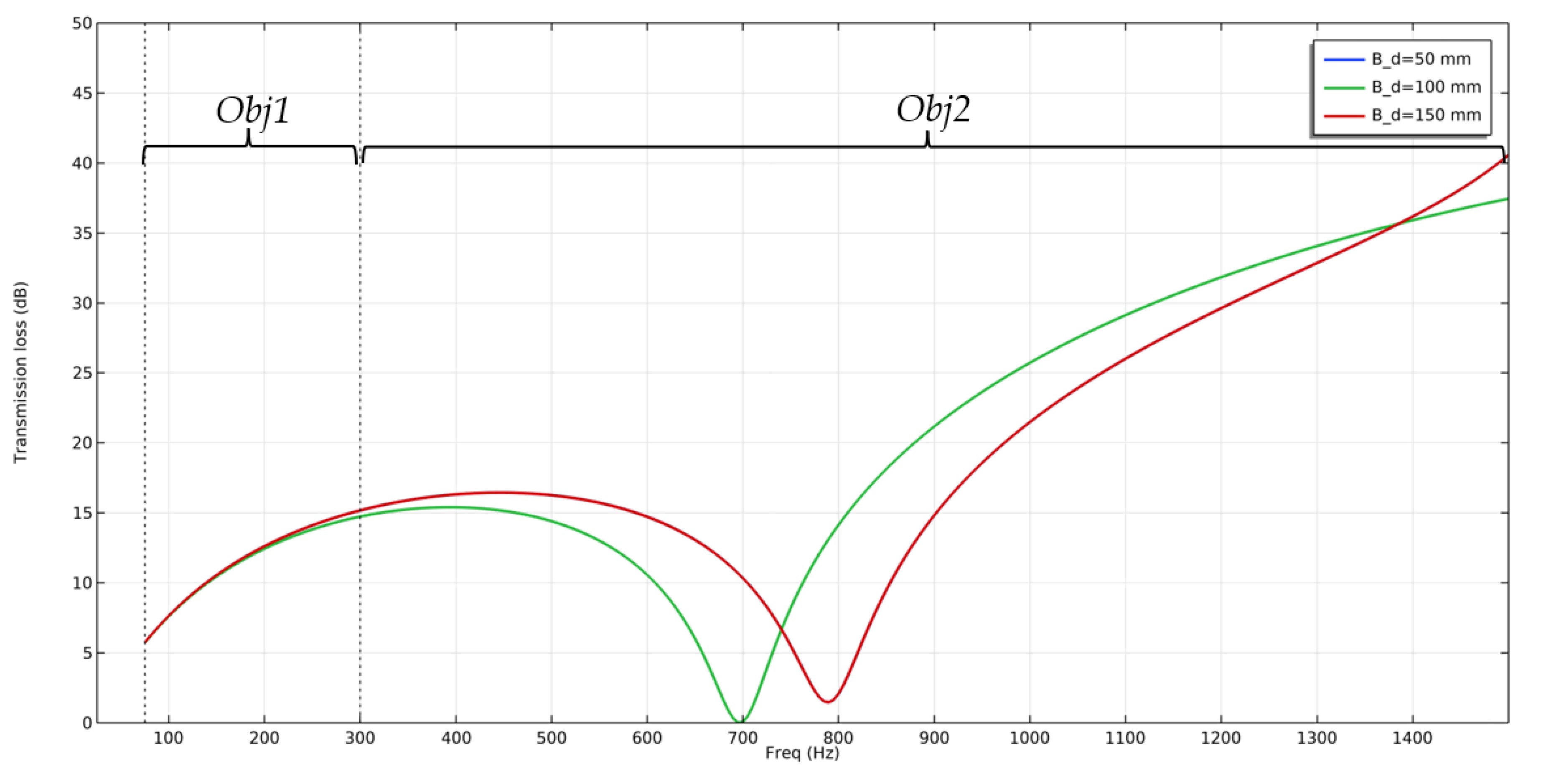
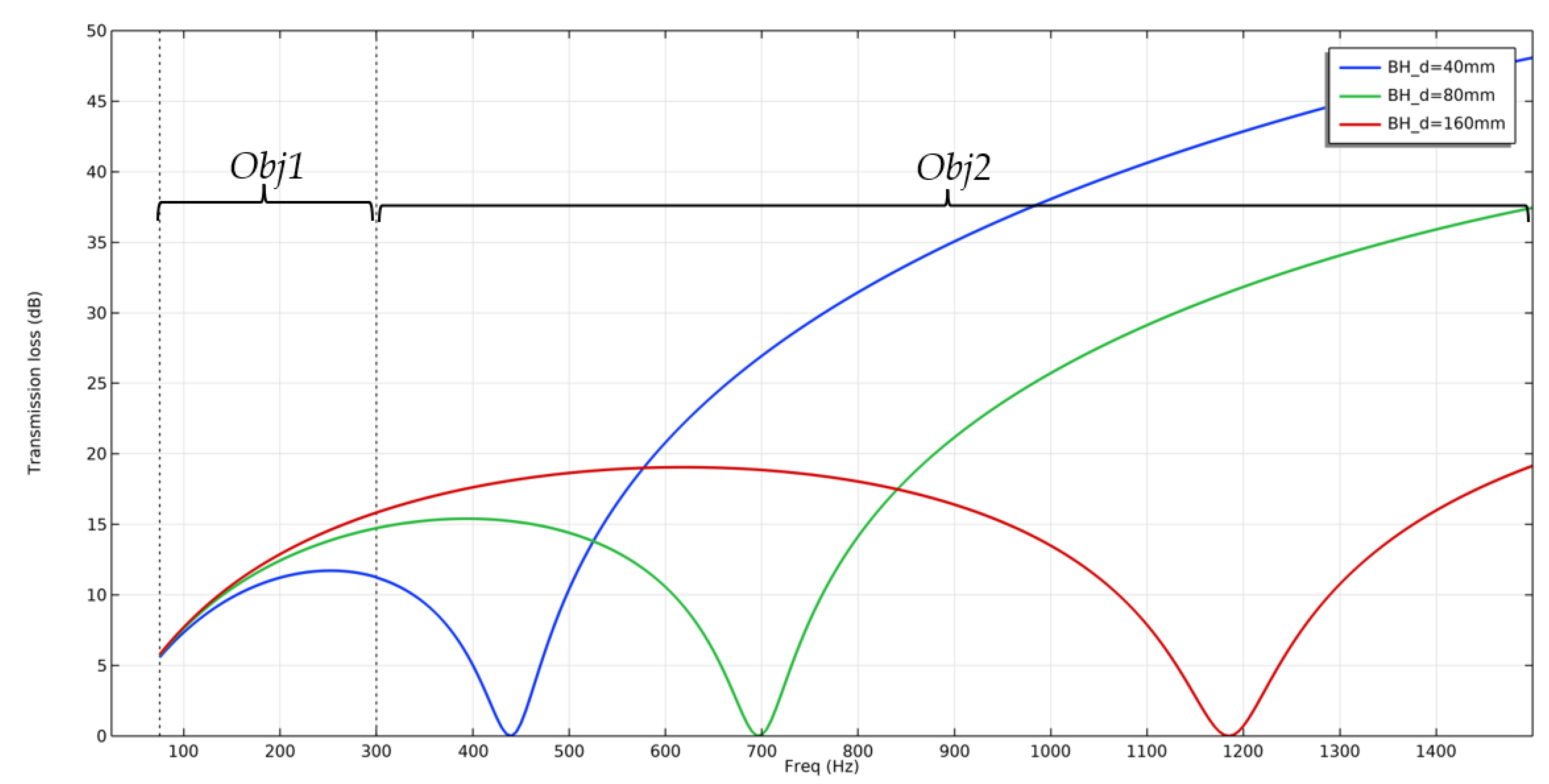
By using this method, the selected design muffler has an improvement against the initial muffler on acoustic performance obj1 and obj2 equal to 0.8% and 98.6%, respectively, and 41.2% enhancement of backpressure in terms of aerodynamic performance assessment. It is observed that acoustic performance assessments are highly dependent on parameter L (length of the muffler), BH_d (baffle hole diameter), and $BIOE\_L$ (baffle inlet outlet extension length) while slightly dependent on $B\_d$ (baffle distance). In addition, backpressure is essentially affected by $L$, $BH\_d,$ and $BH\_o$ (baffle hole offset) and is slightly dependent on $B\_d$.

This work can be extended to consider other features of the muffler, for example adding absorption and perforations, and finding the most suitable options for a desirable muffler with analysis of the muffler performance accordingly. Additionally, this method provides the possibility of evaluating the order of adding features in the tree diagram method and its effect on performance which can save time and costs associated with physical prototyping and testing.

References

1. Gomez, A.V. New Procedure for Loudness Assesment and Noise Attenuation of Ventilation Kitchen Range Hoods. Ph.D. Thesis, Texas A&M University, College Station, TX, USA, 2015. [Google Scholar]
2. Heywood, J. Internal Combustion Engine Fundamentals; Mcgraw-Hill Book, Co.: New York, NY, USA, 1988. [Google Scholar]
3. Denia, F.; Selamet, A.; Martínez, M.; Fuenmayor, F. Sound attenuation of a circular multi-chamber hybrid muffler. Noise Control Eng. J. 2008, 56, 356–364. [Google Scholar] [CrossRef]
4. Jeon, S.; Kim, D.; Hong, C.; Jeong, W. Acoustic performance of industrial mufflers with CAE modeling and simulation. Int. J. Nav. Archit. Ocean. Eng. 2014, 6, 935–946. [Google Scholar] [CrossRef] [Green Version]
5. Zhang, Y.; Wu, P.; Ma, Y.; Su, H.; Xue, J. Analysis on acoustic performance and flow field in the split-stream rushing muffler unit. J. Sound Vib. 2018, 430, 185–195. [Google Scholar] [CrossRef]
6. Tutunea, D.; Calbureanu, M.; Lungu, M. The computational fluid dynamics (CFD) study of fluid dynamics performances of a resistance muffler. Int. J. Mech. 2013, 7, 401–408. [Google Scholar]
7. Venkatagiri, B.R.; Raj, S.K.; Kasyap, S.; Kumar, V.G.; Baalamurugan, J.; Alphonse, M. Latest trends in automotive muffler–A review. In AIP Conference Proceedings; AIP Publishing LLC: Melville, NY, USA, 2020; p. 040019. [Google Scholar]
8. Deery, D.; Flanagan, L.; O’Brien, G.; Rice, H.J.; Kennedy, J. Efficient modelling of acoustic metamaterials for the performance enhancement of an automotive silencer. Acoustics 2022, 4, 329–344. [Google Scholar] [CrossRef]
9. Jones, P.; Kessissoglou, N. An evaluation of current commercial acoustic FEA software for modelling small complex muffler geometries: Prediction vs experiment. In Proceedings of the ACOUSTICS; Australian Acoustical Society: Busselton, Australia, 2009. [Google Scholar]
10. Kalita, U.; Singh, M. Optimization of a reactive muffler used in four-cylinder petrol engine into hybrid muffler by using CFD analysis. Mater. Today Proc. 2022, 50, 1936–1945. [Google Scholar] [CrossRef]
11. Raj, C.M.; Padmavathy, S.; Gokulnath, M.; Kumar, M.S.; Pragadheesh, L. Analysis of Various Automotive Mufflers: Computational Fluid Dynamics Approach. Rev. Geintec-Gest. Inov. Tecnol. 2021, 11, 1339–1348. [Google Scholar]
12. Kumar, S.D.; Praveenkumar, N.; Arulkumar, S.; Boopalan, N.; Praveenkumar, S. Design and Analysis of a Muffler for Engine Exhaust Noise and Heat Reduction; SAE Technical Paper; SAE International: Warrendale, PA, USA, 2021. [Google Scholar]
13. CM, J.; CP, S.K. General Design Principles of Reactive Mufflers: A Review; SSRN: Amsterdam, The Netherlands, 2022. [Google Scholar]
14. Panigrahi, S.; Munjal, M. Combination mufflers-Theory and parametric study. Noise Control Eng. J. 2005, 53, 247–255. [Google Scholar] [CrossRef]
15. Ranjbar, M.; Alinaghi, M. Effect of liner layer properties on noise transmission loss in absorptive mufflers. Math. Model. Appl. 2016, 1, 46–54. [Google Scholar]
16. Nag, S.; Gupta, A.; Dhar, A. Effect of geometric parameters on the acoustical performance of single inlet single outlet expansion chamber muffler. In Proceedings of the 2016 International Conference on Electrical, Electronics, and Optimization Techniques (ICEEOT), Chennai, India, 3–5 March 2016; pp. 2522–2526. [Google Scholar]
17. Amuaku, R.; Asante, E.A.; Edward, A.; Gyamfi, G.B. Effects of chamber perforations, inlet and outlet pipe diameter variations on transmission loss characteristics of a Muffler using Comsol multiphysics. Appl. Sci 2019, 4, 104. [Google Scholar] [CrossRef]
18. Kulkarni, M.; Ingle, R. Effect of Extended Inlet and Outlet Lengths on Transmission Loss of Double Expansion Chamber Reactive Muffler. Int. J. Veh. Struct. Syst. 2022, 14, 135–137. [Google Scholar] [CrossRef]
19. Shah, S.; Kuppili, S.; Hatti, K.; Thombare, D. A Practical Approach towards Muffler Design, Development and Prototype Validation; SAE Technical Paper; SAE international: Warrendale, PA, USA, 2010; Volume 32, p. 0021. [Google Scholar]
20. Munjal, M.; Kumar, V. Design and Analysis of a Plug-Muffler Modified for Low Back-Pressure and Improved Acoustic Performance. SAE Int. J. Veh. Dyn. Stab. NVH 2017, 1, 44–57. [Google Scholar] [CrossRef]
21. Prajapati, V.D.; Desai, A.J. Design and analysis of automotive muffler. Int. J. Eng. Res. Technol. 2016, 5, 384–389. [Google Scholar]
22. Praveen, V.V.; Sethupathi, P.B. Active Muffler for Single Cylinder Engine, Using Electronic Throttle Control for Formula Student Cars; SAE Technical Paper; SAE International: Warrendale, PA, USA, 2017. [Google Scholar]
23. Middelberg, J.; Barber, T.; Leong, S.; Byrne, K.; Leonardi, E. CFD analysis of the acoustic and mean flow performance of simple expansion chamber mufflers. In Proceedings of the ASME International Mechanical Engineering Congress and Exposition, Anaheim, CA, USA, 13–19 November 2004; pp. 151–156. [Google Scholar]
24. Moret, B.M. Decision trees and diagrams. ACM Comput. Surv. CSUR 1982, 14, 593–623. [Google Scholar] [CrossRef]
25. Aksyonov, K.; Antonova, A. Application of the process parameter analysis tree for technological process analysis. In Proceedings of the 2018 Ural Symposium on Biomedical Engineering, Radioelectronics and Information Technology (USBEREIT), Yekaterinburg, Russia, 7–8 May 2018; pp. 212–215. [Google Scholar]
26. Barbieri, R.; Barbieri, N. Finite element acoustic simulation based shape optimization of a muffler. Appl. Acoust. 2006, 67, 346–357. [Google Scholar] [CrossRef]
27. Azevedo, F.; Moura, M.; Vicente, W.; Picelli, R.; Pavanello, R. Topology optimization of reactive acoustic mufflers using a bi-directional evolutionary optimization method. Struct. Multidiscip. Optim. 2018, 58, 2239–2252. [Google Scholar] [CrossRef]
28. Kalita, U.; Saha, P.; Kaberwal, H.S.; Mishra, A.K.; Alam, M.M.; Kadiyala, N. Of an automobile muffler using computational fluid dynamics analysis. JETIR 2021, 8, 11–19. [Google Scholar]
29. Shen, C.; Hou, L. Comparison of various algorithms for improving acoustic attenuation performance and flow characteristic of reactive mufflers. Appl. Acoust. 2017, 116, 291–296. [Google Scholar] [CrossRef]
30. Kashikar, A.; Suryawanshi, R.; Sonone, N.; Thorat, R.; Savant, S. Development of muffler design and its validation. Appl. Acoust. 2021, 180, 108132. [Google Scholar] [CrossRef]
31. Dixit, M.; Sundaram, V. Optimization of Muffler Acoustics Performance Using Dfss Approach; SAE Technical Paper; SAE International: Warrendale, PA, USA, 2016. [Google Scholar]
32. Mimani, A.; Kirby, R. Design of large reactive silencers for industrial applications. In Proceedings of the InterNoise, Chicago, IL, USA, 26–29 August 2018; pp. 26–29. [Google Scholar]
33. Munjal, M.L. Acoustics of Ducts and Mufflers with Application to Exhaust and Ventilation System Design; John Wiley & Sons: Hoboken, NJ, USA, 1987. [Google Scholar]
34. Fang, J.; Zhou, Y.; Jiao, P.; Ling, Z. Study on pressure loss for a muffler based on CFD and experiment. In Proceedings of the 2009 International Conference on Measuring Technology and Mechatronics Automation, Zhangjiajie, China, 11–12 April 2009; pp. 887–890. [Google Scholar]
35. Diesel, G.B.F.-S.M. CFD analysis on the effects of exhaust backpressure generated by four-stroke marine diesel generator after modification of silencer and exhaust flow design. ARPN J. Eng. Appl. Sci. 2006, 12, 1271–1280. [Google Scholar]
36. Potente, D. General design principles for an automotive muffler. In Proceedings of the ACOUSTICS; Australian Acoustical Society: Busselton, Australia, 2005; pp. 153–158. [Google Scholar]
37. Dube, P.; Sajanpawar, P. Study of Perforated Mufflers of Circular and Elliptical cross Sections Using Parametric Technique and Finite Element Methodology; SAE Technical Paper; SAE International: Warrendale, PA, USA, 2007. [Google Scholar]
38. Yang, C.; George, J.; Wahl, T.; Jin, H. Application of shell vibration theory to automotive muffler design and development. Noise Control Eng. J. 2010, 58, 371–381. [Google Scholar] [CrossRef]
39. Mimani, A. Acoustic Analysis and Design of Short Elliptical End-Chamber Mufflers; Springer: Berlin/Heidelberg, Germany, 2021. [Google Scholar]
40. Denia, F.; Albelda, J.; Fuenmayor, F.; Torregrosa, A. Acoustic behaviour of elliptical chamber mufflers. J. Sound Vib. 2001, 241, 401–421. [Google Scholar] [CrossRef]
41. Rao, P.C.; Varma, B.M.; Rao, L. Muffler design, development and validation methods. Int. J. Innov. Res. Sci. Eng. Technol. 2016, 5, 8626–8639. [Google Scholar]
42. Chaudhari, K.C.; Patil, R.; Suryawanshi, N.; Chaudhari, S. Investigation of geometrical parameter on performance of muffler using CFD analysis. Int. Res. J. Eng. Technol. 2016, 3, 1332–1338. [Google Scholar]
43. Srinivas, P.; Mamilla, V.R.; Rao, G.L.N.; Ahmed, S.M. Design and Analysis of an Automobile Exhaust Muffler. Ind. Syst. Eng. 2016, 1, 10–15. [Google Scholar]
44. COMSOL Multiphysics. Acoustics Module User Guide Version 5.4; User’s Man. 2011, p. 169. Available online: https://cn.comsol.com (accessed on 12 June 2023).
45. Kheybari, M.; Ebrahimi-Nejad, S. Dual-target-frequency-range stop-band acoustic metamaterial muffler: Acoustic and CFD approach. Eng. Res. Express 2021, 3, 035027. [Google Scholar] [CrossRef]
46. Barua, S.; Chatterjee, S. CFD analysis on an elliptical chamber muffler of a CI engine. Int. J. Heat Technol. 2019, 37, 613–619. [Google Scholar] [CrossRef] [Green Version]
47. Ferrándiz, B.; Denia, F.; Martínez-Casas, J.; Nadal, E.; Ródenas, J.J. Topology and shape optimization of dissipative and hybrid mufflers. Struct. Multidiscip. Optim. 2020, 62, 269–284. [Google Scholar] [CrossRef]
48. Munjal, M.L. Acoustics of Ducts and Mufflers; Wiley: Hoboken, NJ, USA, 2014. [Google Scholar]
49. Elsayed, A.; Bastien, C.; Jones, S.; Christensen, J.; Medina, H.; Kassem, H. Investigation of baffle configuration effect on the performance of exhaust mufflers. Case Stud. Therm. Eng. 2017, 10, 86–94. [Google Scholar] [CrossRef]
Figure 1. Simulation model definition of the mufflers.
Metrology 03 00015 g001
Figure 2. Muffler mesh for simulations: (a) acoustic mesh and (b) CFD mesh.
Metrology 03 00015 g002
Figure 3. Muffler’s overall length parameter.
Metrology 03 00015 g003
Figure 4. Effect of Length L on TL and comparison with analytical published data (dashed lines).
Metrology 03 00015 g004
Figure 5. CFD simulation for different values of L in muffler. (a) L = 200   m m ; (b) L = 400   m m ; (c) L = 600   m m .
Metrology 03 00015 g005
Figure 6. Sample tree diagram format for methodological analysis.
Metrology 03 00015 g006
Figure 7. Different parameters in baffle. (a) Baffle distance, B_d; (b) baffle hole diameter, BH_d; (c) baffle hole offset, BH_o.
Metrology 03 00015 g007
Figure 8. Different configurations of parameter B_d: (a) 50 mm; (b) 100 mm; (c) 150 mm.
Metrology 03 00015 g008
Figure 9. Effect of baffle distance on TL.
Metrology 03 00015 g009
Figure 10. CFD simulation for different values of B _ d in muffler. (a) B _ d = 50 mm (b) B d = 100 mm; (c) B _ d = 150 mm and the dashed circles for specifying the highest pressure areas.
Metrology 03 00015 g010
Figure 11. Geometry of different values of B H _ d : (a) 40 mm; (b) 80 mm; (c) 160 mm.
Metrology 03 00015 g011
Figure 12. Effect of baffle hole diameter on TL.
Metrology 03 00015 g012
Figure 13. CFD simulation for different values of B H _ d in muffler. (a) B H _ d = 40   m m ; (b)   B H _ d = 80   m m ; (c) B H _ d = 160   m m and the dashed circles for specifying the highest pressure areas.
Metrology 03 00015 g013
Figure 14. Effect of hole offset on TL. Offset hole is (a) 25 mm; (b) 50 mm; (c) 75 mm.
Metrology 03 00015 g014
Figure 15. Effect of baffle hole offset on TL.
Metrology 03 00015 g015
Figure 16. CFD simulation for different values of B H _ o in muffler. (a) B H _ o = 20   m m ; (b)   B H _ o = 40   m m ; (c) B H _ o = 60   m m and the dashed circles for specifying the highest pressure areas.
Metrology 03 00015 g016
Figure 17. Different parameters for extension tube length. (a) Inlet and outlet extension length ( I O E _ L ) with baffle; (b) inlet and outlet baffle extension length ( B I O E _ L ); (c) inlet and outlet extension length ( I O E _ L ) without baffle.
Metrology 03 00015 g017
Figure 18. Effect of inlet and outlet extension length in muffler with baffle on TL.
Metrology 03 00015 g018
Figure 19. CFD simulation for different values of I O E _ L in muffler. (a) I O E _ L = 10 mm; (b) I O E _ L = 40 mm; (c) I O E _ L = 70 mm and the dashed rectangle shows the flow path.
Metrology 03 00015 g019
Figure 20. Effect of baffle hole extension length on TL.
Metrology 03 00015 g020
Figure 21. CFD simulation for different values of B I O E _ L in muffler. (a) B I O E _ L = 10   m m ; (b)   B I O E _ L = 40   m m ; (c) B I O E _ L = 70   m m .
Metrology 03 00015 g021
Figure 22. Effect of inlet and outlet extension length in muffler without baffle on TL.
Metrology 03 00015 g022
Figure 23. CFD simulation for different values of I O E _ L in muffle without baffle. (a) I O E _ L = 10 mm; (b) I O E _ L = 40 mm; (c) I O E _ L = 70 mm.
Metrology 03 00015 g023
Figure 24. Tree diagram of simulation results. L: length of muffler, B_d: baffle distance, BH_d: baffle hole diameter, BH_o: baffle hole offset, IOE_L: inlet and outlet extension length, BIOE_L: baffle inlet and outlet extension length. The corresponding color for initial, a1, b1, b2, and b3 states are purple, green, red, blue, and yellow, respectively.
Metrology 03 00015 g024