The Obtainable Uncertainty for the Frequency Evaluation of Tones with Different Spectral Analysis Techniques

Abstract

Spectral analysis is successfully adopted in several fields. However, the requirements and the constraints of the different cases may be so varied that not only the tuning of the analysis parameters but also the choice of the most suitable technique can be a difficult task. For this reason, it is important that a designer of a measurement system for spectral analysis has knowledge about the behaviour of the different techniques with respect to the operating conditions. The case that will be considered is the realization of a numerical instrument for the real-time measurement of the spectral characteristics of a multi-tone signal (amplitude, frequency, and phase). For this purpose, different signal processing techniques can be used, that can be classified as parametric or non-parametric methods. The first class includes those methods that exploit the a priori knowledge about signal parameters, such as the spectral shape of the signal to be processed. Thus, a self-configuring procedure based on a parametric algorithm should include a preliminary evaluation of the number of components. The choice of the right method among several proposals in the literature is fundamental for any designer and, in particular, for the developers of spectral analysis software, for real-time applications and embedded devices where time and reliability constrains are arduous to fulfil. Different aspects should be considered: the desired level of accuracy, the available elaboration resources (memory depth and processing speed), and the signal parameters. The present paper details a comparison of some of the most effective methods available in the literature for the spectral analysis of signals (IFFT-2p, IFFT-3p, and IFFTc, all based on the use of an FFT algorithm, while improving the spectral resolution of the DFT with interpolation techniques and three parametric algorithms—MUSIC, ESPRIT, and IWPA). The methods considered for the comparison will be briefly described, and references to literature will be given for each one of them. Then, their behaviour will be analysed in terms of systematic contribution and uncertainty on the evaluated frequencies of the spectral tones of signals created from superimposed sinusoids and white Gaussian noise.

1. Introduction

The spectral analysis of signals is successfully adopted in several fields—from electrical [1,2] to typical industrial fields—for speed and fault detection on motors and bearings [3,4,5] in military applications [6], submarine applications [7], and medical applications [8]. Despite the adaptability of frequency analysis for varied applications [9], similar cases might require different approaches, requirements, and constraints; for this reason, they differ in the tuning of the analysis parameters, and the choice of the most suitable technique can be a difficult task to accomplish. For this reason, the designer of a measurement system for spectral analysis must have knowledge about the behaviour of the different techniques concerning the operating conditions. The case that will be considered is the realisation of a numerical instrument for the real-time measurement of the spectral components of a signal: amplitude, frequency, and phase.

For this purpose, different signal processing techniques can be used that can be generally classified in parametric and non-parametric methods. The first class includes those methods that exploit the a priori knowledge about the signal parameters, such as the number of signal spectral components. Thus, a self-configuring procedure based on a parametric algorithm should include a preliminary evaluation of the number of components. The choice of the proper method among the several available approaches is fundamental for designing a procedure based on signal spectral analysis. Different aspects should be considered: the desired level of accuracy, the available elaboration resources (memory depth and processing speed), and the signal nature.

This paper will compare the most effective methods available in the literature for the spectral analysis of signals [10,11,12,13,14,15,16,17,18,19,20,21,22,23,24,25]. The considered methods for the comparison will be briefly described, and references from the literature will be given for each one of them. Their behaviour will be analysed in terms of obtainable uncertainty on the frequency evaluation. Residual errors and repeatability of the measured frequency directly influence the uncertainty of other tone properties, such as phase and amplitude.

The procedure and the criteria adopted for the comparison are described and, eventually, the results are reported and commented upon. Numerical simulations have been run in conditions similar to the real-world operation of a measurement system by studying the effects of added Gaussian noise or quantisation noise to the signal, and their results are shown in this article.

2. Considered Methods

In this section, the algorithms considered for the comparison will be briefly described. At first, some non-parametric algorithms will be presented (IFFT-2p, IFFT-3p, IFFTc), they are all based on the use of a fast Fourier transform (FFT) algorithm, but they improve the spectral resolution of the discrete Fourier transform (DFT) algorithm, with interpolation techniques. Then three parametric algorithms will be introduced (MUSIC, ESPRIT, and IWPA), based on approaches different from the DFT evaluation. Since almost any signal can be represented as a multi-tone signal (1), composed of the sum of $N_s$ sinusoids with amplitude, $A_i$, and phase, ${\varphi }_i$; all the algorithms will be compared with respect to this signal family.

$$x\left(t\right)=\sum _{i=1}^{N_s}{A}_{i}sin(2\pi f_{i}t+{\varphi }_i).$$

(1)

2.1. Non-Parametric Methods

Considering the multi-tone signal in (1), sampled with a $T_s$ sampling period, the obtained signal is described by:

$$x\left(n\right)=\sum _{i=1}^{N_s}{A}_{i}sin(2\pi f_{i}n{T}_s+{\varphi }_i)n=1\dots N.$$

(2)

Non-parametric methods are based on the DFT algorithm, where the spectrum samples are evaluated as follows:

$$X\left(k\right)=\frac{1}{G}\sum _{n=0}^{N-1}w\left(n\right)x\left(n\right)e^{-\frac{2j\pi }{N}kn}k=0\dots N-1,$$

(3)

where $x\left(n\right)$ is the sampled signal (2) and $w\left(n\right)$ are the window samples with gain G, and k is the spectral bin index, also known as the bin number. If the sampled signal is coherent with the module of the sampled sequence DFT (3), then $M\left(k\right)=\left|X\right(k\left)\right|$ presents $N_s$ peaks, corresponding to the $N_s$ tone frequencies; the i-th peak is located exactly at index $k_i$.

When coherent sampling conditions are not assured, a quantization error arises in the frequency estimation [26]; the tone module is underestimated because of the spectral leakage. Moreover, harmonic interference is present, causing an error in parameters estimation when the sampled signal presents two tones with a small frequency difference compared with the frequency resolution, or when it has only one tone but the frequency is less than two times the frequency resolution $\Delta f$.

To correct errors on frequency estimation, phase, and amplitude estimation, several non parametric methods have been exploited in the literature [10]. In the following sections, some non parametric methods will be briefly treated, in particular the interpolated FFT (IFFT) on two points and three points, and the corrected IFFT.

2.1.1. IFFT-2p

Interpolated FFT algorithms [10,11] have been known in the literature for several years, and those based on a two-point interpolation are the most common. The frequency, $f_i$, of the i-th tone can be evaluated as: $f_i=(k_i+{\delta }_i)\Delta f$, where $\Delta f$ is the DFT frequency resolution ($\Delta f=f_s/N$), k is the integer part of the bin ($f/\Delta f$), and ${\delta }_i\in [-1/2,+1/2]$ is the fractional bin deviation. The fractional bin deviation, ${\delta }_i$, is evaluated from the ratio between the two largest samples closest to the peak: ${\alpha }_i=\frac{\left|X\right(k_i+{ϵ}_i\left)\right|}{\left|X\right(k_i\left)\right|}$, where: ${ϵ}_i=sign\left(\right|X(k_i+1)|-|X(k_i-1)\left|\right)$. Considering the sampled spectrum of the window function, $W\left(k\right)$, the following is obtained [9]:

$${\alpha }_i=\frac{\left|W\right({ϵ}_i-{\delta }_i\left)\right|}{\left|W\right(-{\delta }_i\left)\right|}=\frac{\left|W\right(k_i-{\delta }_i\left)\right|}{\left|W\right(k_i\left)\right|}$$

(4)

The value of ${\delta }_i$ can be evaluated from the latter relationship, given the window function and its analytical expression.

2.1.2. IFFT-3p

The interpolated three-point DFT algorithm [12,13,14,15] is based on an interpolation of the DFT results of the signal, windowed by cosine windows, and using three points for each tone peak. Considering the multi-tone signal, with $N_s$ spectral components of (1), like the IFFT-2p, the frequency $f_i$ of the i-th tone is evaluated as $f_i=(k_i+{\delta }_{3i})\Delta f$; in this case, ${\delta }_{3i}$ is evaluated considering the three largest samples of the peak:

$${\alpha }_{3i}=\frac{|X(k_i-1)|+|X(k_i+1)|}{|X(k_i-1)|+2|X\left(k_i\right)|+|X(k_i+1)|},$$

(5)

$${\delta }_{3i}=K\ast {\alpha }_{3i},$$

(6)

where K is a proportional factor that depends on the used windowing function; in the case of an Hanning window, this is $K=2$.

2.1.3. IFFTc

The corrected interpolated FFT algorithm, presented in [16,17,18], is based on an IFFT-2p, but includes further processing to correct the effects of the harmonic interference between spectral components. Concerning the multi-tone signal of (1), it has been shown that the DFT value closest to the peak of the i-th spectral component can be written as: $X\left(k_i\right)=\frac{V_i}{S}W(-{\delta }_i)+F_i$, where $V_i=\frac{A_i}{2j}{e}^{j{\varphi }_i}$, $S={\sum }_{i=0}^{N-1}w\left(n\right)$, and the contribution of the harmonic interference of other components on the i-th one can be taken into account by the term $F_i$. Similar considerations can be made for the second strongest bin: $X(k_i+{ϵ}_i)=\frac{V_i}{S}W({ϵ}_i-{\delta }_i)+B_i$.

The ${\alpha }_i$ becomes: ${\alpha }_i^{\prime }=\frac{\left|W\right({ϵ}_i-{\delta }_i\left)\right|}{\left|W\right(-{\delta }_i\left)\right|}=\frac{|X(k_i+{ϵ}_i)-B_i|}{|X\left(k_i\right)-F_i|}$. The correction factors, $F_i$ and $B_i$, depend on the frequency, amplitude, and phase of the signal tones. The proposed solution consists of using the values of frequency, amplitude, and phase measured with a preliminary two-point IFFT to evaluate the correction factors (IFFTc). In the presence of a low-frequency tone, the frequency image contribution can be corrected with the same relationships [20]. This step could be iterated further, but without any significant improvement in terms of estimation error reduction.

2.2. Parametric Methods

Numerous parametric methods exist in the literature; however, in this article, only the three algorithms presenting the best compromise in terms of computational requirements and estimation performance have been considered—MUSIC, ESPRIT, and IWPA.

2.2.1. MUSIC

This parametric algorithm (multiple signal classification) [19,20,21] determines the frequencies of the tones in a signal by performing a decomposition of the covariance matrix of the sequence of signal samples, $x\left(n\right)$. We modelled the input data as a $N_s$-tone signal and a superimposed noise, as follows:

$$x\left(n\right)=\sum _{i=i}^{N_s}{A}_{i}sin(2\pi f_{i}n{T}_s+{\varphi }_i)+z\left(n\right),$$

(7)

where $z\left(n\right)$ is the noise signal. The covariance of the signal is $R_x=E\left\{x{x}^H\right\}$, and can be numerically computed using signal samples, $x\left[n\right]$. If the noise is considered to be white Gaussian noise, then the signal can be decomposed in order to separate the signal from the noise orthogonal subspaces. The frequencies of the signal tones can be estimated from this decomposition [19]. To compute the MUSIC algorithm, the number of signal tones, $N_s$, must be known in advance; the same applies to the number of signals eigenvectors to be found with the decomposition.

2.2.2. ESPRIT

This parametric algorithm (estimation of signal parameter via rotational invariance technique), introduced in [22,23,24], exploits the rotational invariance property, which is valid for the signal eigenvectors ($\mathbf{x}$) of the sample sequence covariance matrix. Similar to the MUSIC algorithm, ESPRIT needs an estimation of the signal covariance matrix. Thanks to the knowledge of the number of components, the eigenvectors corresponding to signal components can be separated from the noise eigenvectors. Each signal eigenvector can be written as:

$$\begin{array}{cc}\hfill {\mathbf{x}}_k& =\left[x\right(0),x(1),\dots ,x(N-2),x(N-1\left)\right]\hfill \\ \hfill & ={\mathbf{A}}_{\mathbf{k}}\times [1,e^{j{\omega }_k},e^{j2{\omega }_k},\dots ,e^{j(N-1){\omega }_k}]\hfill \\ \hfill & =[s_1,x(N-1)]=[x\left(0\right),s_2],\hfill \end{array}$$

(8)

where ${\mathbf{A}}_{\mathbf{k}}$ is the coefficients vector. The $s_2=s_1{e}^{j{\omega }_1}$ rotational invariance property is valid, so all the signal eigenvectors and the signal components can be collected into the matrix, U, as well as into the signal components in the following matrices:

$$\begin{array}{cc}\hfill {\Gamma }_1& ={\left[I_{M-1}\right|0_{M-1}]}_{\left(M_1\right)\times M}\end{array}$$

(9a)

$$\begin{array}{cc}\hfill {\Gamma }_2& ={\left[0_{M-1}\right|I_{M-1}]}_{\left(M_1\right)\times M}\end{array}$$

(9b)

Considering the rotational invariance property for each signal eigenvector, the selection matrices, ${\Gamma }_1$ (9a) and ${\Gamma }_2$ (9b), can be used to obtain the following system:

$$\left[{\Gamma }_{1}U\right]\Phi ={\Gamma }_{2}U,$$

(10)

where $\Phi =diag\{e^{j{\omega }_1},e^{j{\omega }_2},\dots ,e^{j{\omega }_{N_s}}\}$. It is possible to obtain the frequencies of the components belonging to the signal solving this system with a least square technique.

2.2.3. IWPA

This method, proposed in [25], is based on the iteration of the weighted phase average algorithm (WPA). Considering the case of a signal with only one spectral component, $x\left(t\right)=A_{0}cos(2\pi f_{0}t+{\varphi }_0)$, a coarse estimation, ${\widehat{f}}_0$, of the frequency, $f_0$, can be obtained in the first place, as the maximum of the amplitude of the DFT sequence, $X\left(k\right)$. The signal is then divided into M non-overlapping segments of length P: $x_s\left(n\right)=x(n+s·P)$, $0\le n\le P-1$.

In the simple but effective case of two segments and $P=N/2$, the spectra of the two segments, $x_1$ and $x_2$, are evaluated at frequency ${\widehat{f}}_0$, and it can be shown that the fractional bin deviation, $\delta$, can be estimated as:

$$\delta =\frac{N}{2\pi ·P}\left(\phase{X_1\left({\widehat{f}}_0\right)}-\phase{X_2\left({\widehat{f}}_0\right)}\right).$$

(11)

The IWPA algorithm, at each iteration, applies the WPA to obtain the frequency estimation of the strongest component, while amplitude and phase of this component are obtained through a least square technique. In the next step, the estimated component is subtracted from the samples of the previous iteration in the time domain. The number of iterations has to be equal to the number of components, so that a new component can be estimated at each iteration. The IWPA algorithm can be easily converted into a non-parametric algorithm by iterating its processing steps until the level of the residual decreases below a threshold.

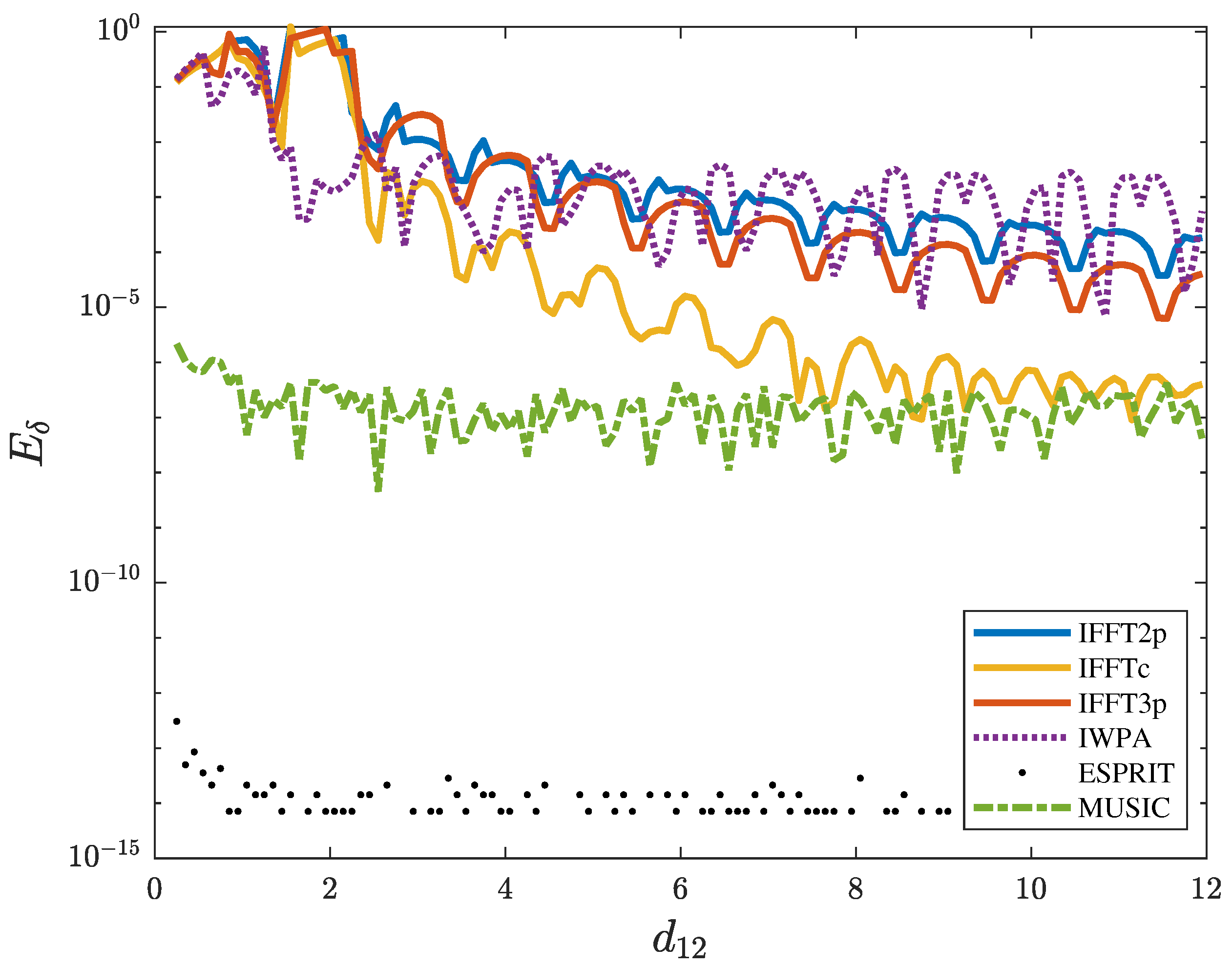
3. Residual Errors

Due to approximations, the considered methods may exhibit a bias between the estimated and actual values of the signal tones, even when noise is not superimposed to the signal, and their expected values are not equal to their actual values. Such behaviour can be associated with interharmonic interference; as for IFFTc and IWPA, the behaviour can be associated with inadequate knowledge of the values required by parametric methods or the finite word length of the data processing.

To evaluate the proposed methods and produce a clear comparison of their performance, the multi-frequency signals described by (1) were considered; the tests are made for different values of the number of tones ($N_s$), the number of samples (N), the frequency ($f_i$), the amplitude ($A_i$), and the phase (${\varphi }_i$). All the simulations have been made supposing an observation window longer than two periods of the signal. The major effects analysed are the frequency resolution, the signal dynamic range, and the harmonic interference [10].

$$\begin{array}{ccc}\hfill f_i& =& (k_i+{\delta }_i)\Delta f\hfill \end{array}$$

(12a)

$$\begin{array}{ccc}\hfill A_i& =& {\beta }_i·A_0\hfill \end{array}$$

(12b)

$$\begin{array}{ccc}\hfill d_{ij}& =& \frac{f_j-f_i}{\Delta f}\hfill \end{array}$$

(12c)

Given Equations (12a)–(12c), where $k_i$ is the frequency bin index corresponding to $f_i$ and ${\delta }_i$ is the fractional bin deviation, the simulations are made at changing values of ${\delta }_i$, $d_{ij}$, ${\beta }_i$, ${\varphi }_i$, and N in order to analyse the dependence of the harmonic interference effects on the signal characteristics and the measurement system settings. In order to evaluate the interference effects on the different methods, tests with only two tones with the same amplitude ($A_1=A_2$), corresponding to more substantial interference on both tones, refs. [3,4,5] are carried out at changing distances between tones, $d_{12}$; with $d_1$ always greater than 20.

The logarithms of the absolute errors on the fractional bin deviations are calculated as the difference between the measured (${\widehat{\delta }}_i$) and the real value (${\delta }_i$), as follows:

$$E_{{\delta }_i}=|{\widehat{\delta }}_i-\delta i|$$

(13)

In Figure 1 the estimation error (13) for the first tone versus the distance between tones ($d_{12}$) is reported for the considered methods; similar results are obtained with the second tone. Interpolated FFT algorithms use the Hanning window, while for MUSIC and ESPRIT, $M=N/4$ was posed, and the matrix covariance was calculated using the samples with no noise added.

Some considerations can be outlined, as follows:

• For each distance, the best performance is obtained by the ESPRIT method, that exhibits the lowest error at any distance between the tones since the error due to the frequency quantization is negligible.
• When the distance between tones is small ($d_{12}<2\mathrm{bins}$), the non-parametric approaches detect only one tone and the errors on the detected tone are significant (comparable with $\delta$). Even if the IWPA method is able to estimate both tones and its errors are lower than those of the parametric approach, the error is still high.
• The tone distance slightly influences the algorithms based on the autocorrelation (MUSIC and ESPRIT): only for $d_{12}$ lower than one bin is the MUSIC algorithm affected by a highest residual error.
• The performance of IWPA and IFFT are comparable, but for small tone distances, the IWPA gives better estimations—vice versa occurs for larger distances $d_{12}$.
• The IFFTc algorithm for tone distance greater than 8 bin gives results comparable with MUSIC: errors of the order of 10-6 are measured for both tones.

Since parametric algorithms require the knowledge of the number of spectral components, but the information can not be obtained in some applications, a characterization of all the algorithms will be reported for the case in which a different and generally wrong number of spectral components ($N_{s_0}$) is specified. For instance, Figure 2 shows the errors on $\delta$ versus the specified number of tones, $N_{s_0}$, in the case of a five-tone signal ($N_s=5$) for the considered algorithms. The results refer to a signal with all the tones at the same amplitude ($A_i=1$) and uniformly spaced with $d_{i,i-1}=3$. For the cases where $N_{s_0}<5$, the error on $\delta$ for a non-detected tone is evaluated with respect to the closest detected tone.

As expected, the algorithms based on IFFT, being non-parametric algorithms, are not influenced by $N_{s_0}$, and the residual errors are quite similar for each tone. Parametric methods MUSIC and ESPRIT manifest a different behaviour: errors are very high for each tone as long as $N_{s_0}$ is lower than the actual number of tones. In other words, if $N_{s_0}$ is lower than $N_s$, then the estimated frequencies are significantly different (at least $\Delta f/2$) from the actual frequencies of each of the five tones. When $N_{s_0}\ge N_s$, the ESPRIT method gives the best performance: it does not show residual errors, and small differences (less than ${10}^{-15}$) are only caused by the finite word length of the precessing unit (CPU); MUSIC shows greater errors (about ${10}^{-7}$), but these are negligible with respect to the other methods. IWPA is less sensitive to an underestimated number of tones ($N_{s_0}\ge N_s$): in these cases, the frequency estimations are better than the other parametric methods, while for a $N_{s_0}\ge N_s$, its estimation deteriorates, since noise components are considered erroneously as signal tones until $N_{s_0}$ components are detected. In the results of Figure 2, when $N_{s_0}$ is less than $N_s=5$, the errors for the undetected components are evaluated as the absolute difference between the actual value for that component and the estimated value for the closest component.

Further tests were carried out to highlight the sensitivity of the different methods to the number of processed samples; in particular, the trends (not reported here for the sake of brevity) of the errors on ${\delta }_i$, versus the bin distance, and versus the tone amplitudes, do not change when the number of acquired samples changes from 128 to 2048. This is expected for the error on ${\delta }_i$, which is a kind of relative error and is different from the error on the frequency. Once the sampling frequency has been set, the greater the number of samples, the lower the spectral resolution, and, consequentially, the lower the error on frequency will be. However, a small reduction in the residual errors is measured only for the IWPA and IFFT methods when N increases (from about $E_{\delta }=3\times {10}^{-3}$ with $N=128$ to $E_{\delta }=2\times {10}^{-4}$ for $N=4096$).

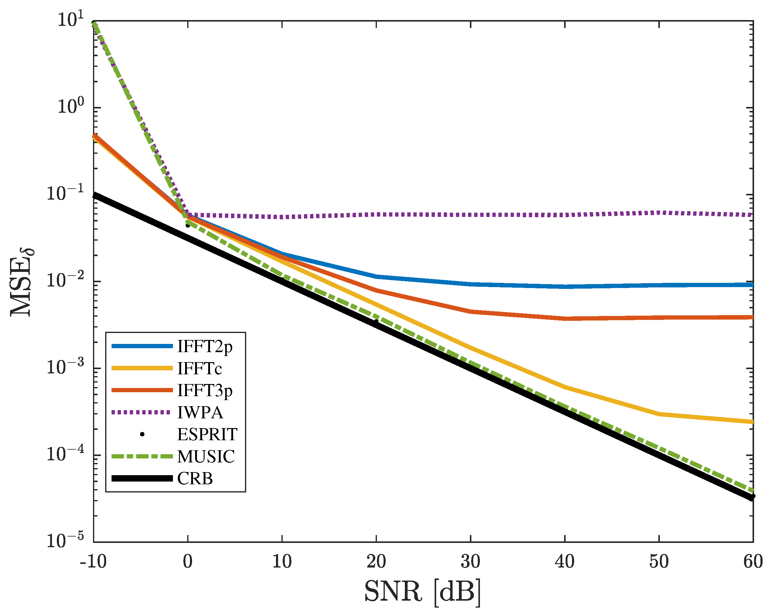
4. Repeatability under Noisy Conditions

Some amount of noise always corrupts real-life signals, so the considered methods have to be evaluated when applied with noisy signals, since their performance may worsen significantly. The tests are carried out by changing the signal characteristics to estimate each method’s sensitivity to the tone composition; only two-tone signals are considered. Once the signal and the measurement parameters have been fixed, a Gaussian noise is added, noisy signal samples are generated, and the algorithms process these points in order to estimate the signal characteristics. For each signal, configuration, and noise level, the tests are repeated 1000 times; the mean and the standard deviation of the results of the algorithms are calculated. For the three algorithms, based on the FFT interpolation, a Hanning window is used.

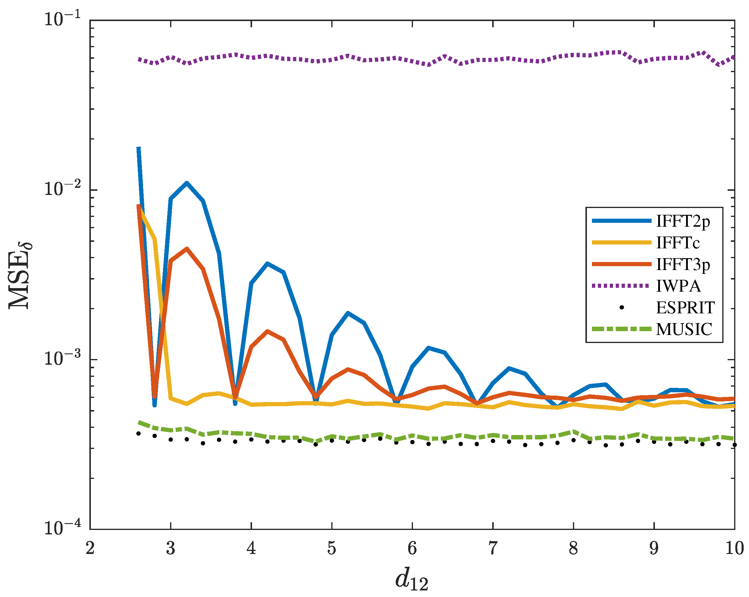
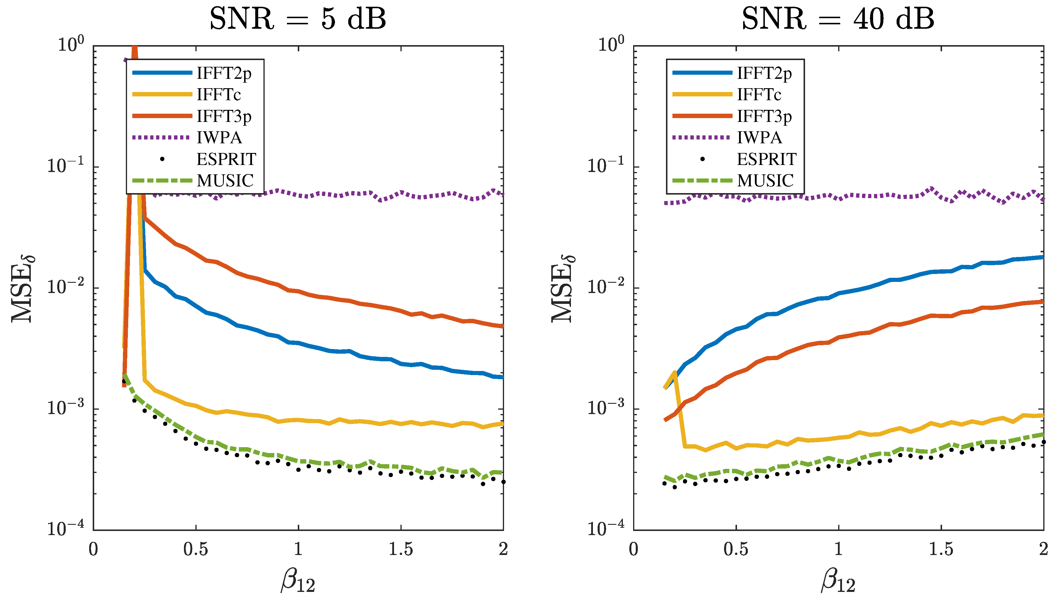
4.1. Sensitivity to the First Tone Distance

Figure 3 reports the behaviour of the algorithms respect to a signal composed of two tones very close in frequency ($d_{12}=3\mathrm{bins}$) and with the same null phase. The measured mean square error (MSE) versus the signal-to-noise ratio (SNR) for the different methods are reported, where the Cramér–Rao bound (CRB) [14] is also reported, since it gives information about the best theoretical performance (minimum variance of the quantity of interest) achievable with an ideal estimator, versus the level of superimposed noise. It has to be highlighted that the MSE considers both the random variability and the systematic effects [13]. The adopted CRB values are obtained with relationships valid in the specific case of a single-tone signal. However, the CRB estimation can be considered a kind of lower limit, and the goodness of the estimation of a proposed method can be evaluated through the closeness of the resulting MSE to the CRB.

Analysing these results, it is possible to state that IFFT and IFFTc algorithms are less sensitive to a high noise level than the other algorithms. In particular, IFFTc shows an MSE on $\delta$ less than 0 dB for SNR less than zero, while the errors can reach 20 dB for the other algorithms. For higher SNR, MUSIC, and ESPRIT show the best performance, but the results of IFFTc and IWPA are comparable with those of the other two methods when the phases are equal to zero. In presence of phase difference, not reported here for simplicity, the performance of ESPRIT and MUSIC does not change while IFFT deteriorates slightly (about 2 dB) for SNR values between 0 dB and 20 dB; the MSE on $\delta$ of the IFFTc algorithm declines of about 3 dB for high SNR (greater than 40 dB) when residual systematic effects on the phase estimation become predominant, and IWPA remarkably loses its estimation capability at the point that it can hardly be adopted.

Figure 4 reports the MSE on $\delta$ versus the relative distance between the two tones of a signal. The improvement of interpolation of the IFFTc over IFFTs is evident since IFFTc keeps good performance from $d_{12}$ equal to 3 onwards. However, the lowest values of ${\mathrm{MSE}}_{\delta }$ are reached by ESPRIT and MUSIC.

4.2. Sensitivity to the Tone–Amplitude Ratio

In Figure 5 the trends of the MSE in the estimation of the bin deviations for a two-tone signal with very close frequencies ($d_{12}=3$) and with random phases are reported, versus the amplitude of the second tone (${\beta }_2$ changes in the range $[0.1,2]$, while ${\beta }_1=1$) for two different SNRs (5 dB and 40 dB). The figures show only the performance of the parametric method ESPRIT and the non-parametric algorithm based on IFFT, since the results of MUSIC are very similar to those of ESPRIT, while IWPA introduces very high errors in presence of phase variations.

ESPRIT algorithm exhibits worse performance in the estimation of the the second tone frequency when ${\beta }_2$ is low, due to the low values of SNR at the second tone especially in the case of the lowest of the two SNR values (5 dB), while the MES value decreases for increasing amplitudes of the second tone. The estimation of the highest tone is not influenced by the amplitude of the lowest one. On the other hand, the IFFTc method is slightly influenced by the change in amplitude. Moreover, the variability obtained with all the methods on ${\delta }_i$ is comparable (IFFTc is characterized by a standard deviation ${\sigma }_{{\delta }_i}$ a bit greater than the others) and the same behaviour is observed when the second tone amplitude becomes significantly greater than the noise (${\beta }_2>0.5$).

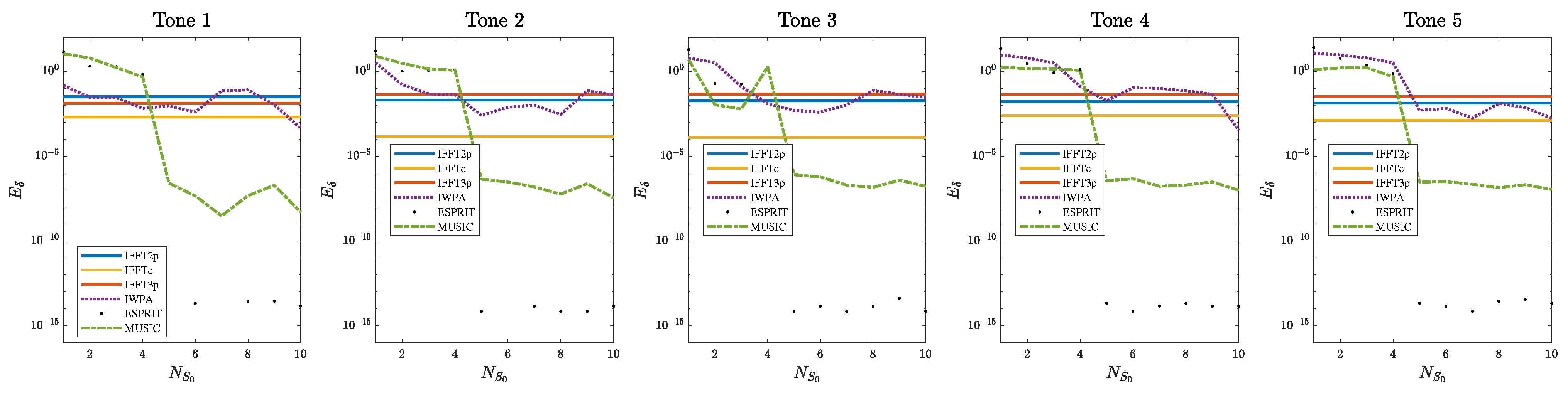
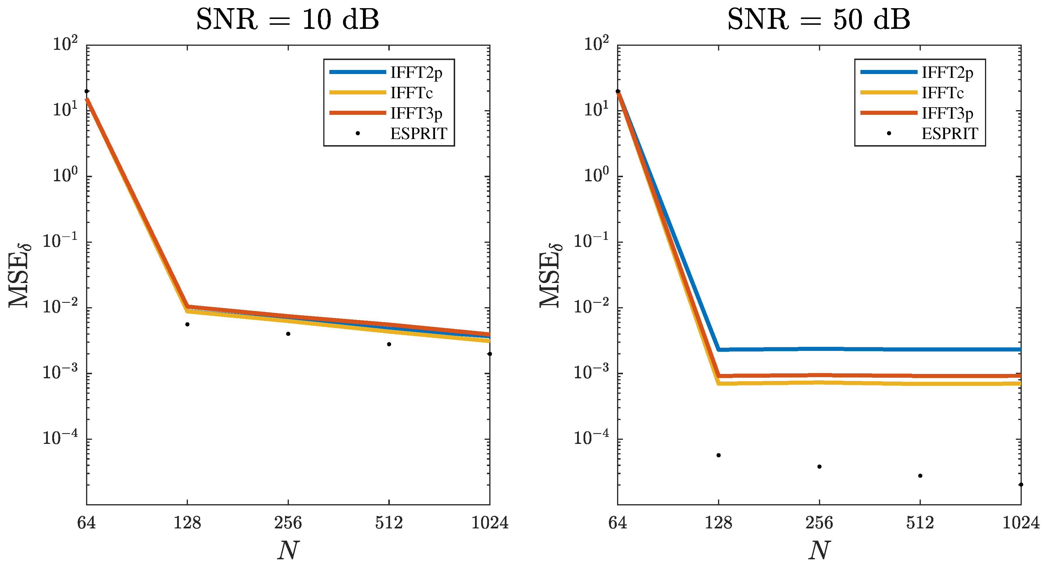
4.3. Sensitivity to the Number of Samples

In Figure 6 the standard deviations of the errors versus N are reported, for a given signal with two tones of the same amplitude and for two different noise levels. As expected, the standard deviations decrease when the number of processed samples increases. For both noise levels, the effect of the tone distance is less significant for high N. In the case of the lowest SNR value (5 dB), the trend is quite the same for all the methods, since the variability due to noise is comparable to the systematic effect of IFFT; meanwhile, for the highest SNR value (40 dB), the parametric algorithms and IFFTc show better performances.

5. Uncertainty Evaluation

As evidenced in Section 3, all the analysed methods present a residual error, that can be negligible or not function depending on the signal characteristics and the processing parameters. The residual contribution cannot be corrected since it strictly depends on the signal characteristics and the uncertainty evaluation has to be taken into account. To this aim, it is possible to write the following:

$$\delta ={\delta }_m+C_{\delta },$$

(14)

where $\delta$ is the corrected bin value, ${\delta }_m$ is the evaluated bin value, and $C_{\delta }$ is the correction that can be modelled as random variable with mean value equal to zero and standard deviation, ${\sigma }_C$, different from zero. Applying the ISO GUM [27] the measurement uncertainty is equal to:

$$u_{\delta }=\sqrt{{\sigma }_{\delta }^2+{\sigma }_C^2}.$$

(15)

As for the standard deviation of the correction value, the measurement uncertainty can be estimated considering group of signals with similar characteristics. In

Table 1. Measurement uncertainty, $u_{\delta }$, evaluated for two-tone signals with tones at varying distance for different values of ${\beta }_{12}$, changing $d_{12}$ from $d_1$ to $d_2$. The simulations were repeated 1000 times, randomizing the tone phases with a 256-sample signal.

${\mathit{\beta }}_{12}=0.01$
		Tone 1						Tone 2
${\mathit{d}}_{\mathbf{1}}$	${\mathit{d}}_{\mathbf{2}}$	IFFT2p	IFFTc	IFFT3p	IWPA	ESPRIT	MUSIC	IFFT2p	IFFTc	IFFT3p	IWPA	ESPRIT	MUSIC
3	4	6.7 × 10${}^{-5}$	1.5 × 10${}^{-4}$	2.4 × 10${}^{-5}$	1.1 × 10${}^{-3}$	1.1 × 10${}^{-14}$	1.6 × 10${}^{-7}$	-	-	-	1.1 × 10${}^{-1}$	9.6 × 10${}^{-13}$	1.6 × 10${}^{-7}$
4	5	3.0 × 10${}^{-5}$	6.0 × 10${}^{-5}$	9.1 × 10${}^{-6}$	1.1 × 10${}^{-3}$	1.1 × 10${}^{-14}$	1.8 × 10${}^{-7}$	6.6 × 10${}^{-1}$	5.8 × 10${}^{-1}$	6.7 × 10 ${}^{-1}$	1.0 × 10${}^{-1}$	9.3 × 10${}^{-13}$	1.8 × 10${}^{-7}$
5	6	1.6 × 10${}^{-5}$	1.0 × 10${}^{-5}$	4.3 × 10${}^{-6}$	1.1 × 10${}^{-3}$	1.1 × 10${}^{-14}$	1.9 × 10${}^{-7}$	1.2 × 10${}^{-1}$	3.6 × 10${}^{-5}$	5.5 × 10 ${}^{-2}$	1.0 × 10${}^{-1}$	9.9 × 10${}^{-13}$	1.9 × 10${}^{-7}$
6	7	9.5 × 10${}^{-6}$	3.4 × 10${}^{-6}$	2.3 × 10${}^{-6}$	1.1 × 10${}^{-3}$	1.0 × 10${}^{-14}$	1.6 × 10${}^{-7}$	7.7 × 10${}^{-2}$	3.2 × 10${}^{-5}$	2.6 × 10 ${}^{-2}$	1.0 × 10${}^{-1}$	9.9 × 10${}^{-13}$	1.7 × 10${}^{-7}$
7	12	3.5 × 10${}^{-6}$	5.6 × 10${}^{-7}$	6.7 × 10${}^{-7}$	1.1 × 10${}^{-3}$	1.0 × 10${}^{-14}$	1.7 × 10${}^{-7}$	2.9 × 10${}^{-2}$	2.8 × 10${}^{-5}$	7.4 × 10 ${}^{-3}$	1.0 × 10${}^{-1}$	9.4 × 10${}^{-13}$	1.7 × 10${}^{-7}$
12	20	7.8 × 10${}^{-7}$	1.8 × 10${}^{-7}$	9.4 × 10${}^{-8}$	1.1 × 10${}^{-3}$	1.0 × 10${}^{-14}$	1.7 × 10${}^{-7}$	6.5 × 10${}^{-3}$	2.2 × 10${}^{-5}$	9.8 × 10 ${}^{-4}$	9.7 × 10${}^{-2}$	9.3 × 10${}^{-13}$	1.7 × 10${}^{-7}$
${\mathbf{\beta }}_{\mathbf{12}}=\mathbf{0.1}$
		Tone 1						Tone 2
${\mathit{d}}_{\mathbf{1}}$	${\mathit{d}}_{\mathbf{2}}$	IFFT2p	IFFTc	IFFT3p	IWPA	ESPRIT	MUSIC	IFFT2p	IFFTc	IFFT3p	IWPA	ESPRIT	MUSIC
3	4	6.8 × 10${}^{-4}$	2.3 × 10${}^{-4}$	2.4 × 10${}^{-4}$	1.3 × 10${}^{-3}$	1.1 × 10${}^{-14}$	1.6 × 10${}^{-7}$	5.3 × 10${}^{-2}$	2.3 × 10${}^{-4}$	3.5 × 10${}^{-2}$	1.0 × 10${}^{-1}$	1.2 × 10${}^{-14}$	1.6 × 10${}^{-7}$
4	5	3.0 × 10${}^{-4}$	3.8 × 10${}^{-5}$	9.1 × 10${}^{-5}$	1.2 × 10${}^{-3}$	1.1 × 10${}^{-14}$	1.8 × 10${}^{-7}$	2.4 × 10${}^{-2}$	4.1 × 10${}^{-5}$	1.2 × 10${}^{-2}$	1.0 × 10${}^{-1}$	1.2 × 10${}^{-14}$	1.8 × 10${}^{-7}$
5	6	1.6 × 10${}^{-4}$	9.9 × 10${}^{-6}$	4.3 × 10${}^{-5}$	1.2 × 10${}^{-3}$	1.1 × 10${}^{-14}$	1.9 × 10${}^{-7}$	1.3 × 10${}^{-2}$	1.2 × 10${}^{-5}$	5.2 × 10${}^{-3}$	1.0 × 10${}^{-1}$	1.2 × 10${}^{-14}$	1.9 × 10${}^{-7}$
6	7	9.5 × 10${}^{-5}$	3.4 × 10${}^{-6}$	2.3 × 10${}^{-5}$	1.2 × 10${}^{-3}$	1.1 × 10${}^{-14}$	1.6 × 10${}^{-7}$	7.8 × 10${}^{-3}$	5.3 × 10${}^{-6}$	2.6 × 10${}^{-3}$	1.0 × 10${}^{-1}$	1.3 × 10${}^{-14}$	1.7 × 10${}^{-7}$
7	12	3.6 × 10${}^{-5}$	6.0 × 10${}^{-7}$	7.0 × 10${}^{-6}$	1.1 × 10${}^{-3}$	1.1 × 10${}^{-14}$	1.7 × 10${}^{-7}$	3.1 × 10${}^{-3}$	3.0 × 10${}^{-6}$	7.9 × 10${}^{-4}$	9.3 × 10${}^{-2}$	1.2 × 10${}^{-14}$	1.7 × 10${}^{-7}$
12	20	1.9 × 10${}^{-6}$	1.9 × 10${}^{-7}$	1.5 × 10${}^{-7}$	1.1 × 10${}^{-3}$	1.1 × 10${}^{-14}$	1.6 × 10${}^{-7}$	1.6 × 10${}^{-4}$	1.4 × 10${}^{-6}$	1.5 × 10${}^{-5}$	9.7 × 10${}^{-2}$	1.3 × 10${}^{-14}$	1.6 × 10${}^{-7}$
${\mathbf{\beta }}_{\mathbf{12}}=\mathbf{1.0}$
		Tone 1						Tone 2
${\mathit{d}}_{\mathbf{1}}$	${\mathit{d}}_{\mathbf{2}}$	IFFT2p	IFFTc	IFFT3p	IWPA	ESPRIT	MUSIC	IFFT2p	IFFTc	IFFT3p	IWPA	ESPRIT	MUSIC
3	4	6.8 × 10${}^{-3}$	2.3 × 10${}^{-4}$	2.4 × 10${}^{-3}$	4.0 × 10${}^{-3}$	1.1 × 10${}^{-14}$	1.6 × 10${}^{-7}$	5.4 × 10${}^{-3}$	2.3 × 10${}^{-4}$	3.5 × 10${}^{-3}$	1.0 × 10${}^{-1}$	1.1 × 10${}^{-14}$	1.6 × 10${}^{-7}$
4	5	3.0 × 10${}^{-3}$	3.8 × 10${}^{-5}$	9.1 × 10${}^{-4}$	4.2 × 10${}^{-3}$	1.0 × 10${}^{-14}$	1.8 × 10${}^{-7}$	2.4 × 10${}^{-3}$	4.1 × 10${}^{-5}$	1.2 × 10${}^{-3}$	1.0 × 10${}^{-1}$	1.1 × 10${}^{-14}$	1.8 × 10${}^{-7}$
5	6	1.6 × 10${}^{-3}$	9.9 × 10${}^{-6}$	4.3 × 10${}^{-4}$	2.9 × 10${}^{-3}$	1.1 × 10${}^{-14}$	1.9 × 10${}^{-7}$	1.3 × 10${}^{-3}$	1.1 × 10${}^{-5}$	5.2 × 10${}^{-4}$	1.0 × 10${}^{-1}$	1.1 × 10${}^{-14}$	1.9 × 10${}^{-7}$
6	7	9.5 × 10${}^{-4}$	3.4 × 10${}^{-6}$	2.3 × 10${}^{-4}$	3.0 × 10${}^{-3}$	1.1 × 10${}^{-14}$	1.7 × 10${}^{-7}$	7.8 × 10${}^{-4}$	4.0 × 10${}^{-6}$	2.6 × 10${}^{-4}$	1.0 × 10${}^{-1}$	1.1 × 10${}^{-14}$	1.7 × 10${}^{-7}$
7	12	3.6 × 10${}^{-4}$	7.3 × 10${}^{-7}$	7.0 × 10${}^{-5}$	2.2 × 10${}^{-3}$	1.1 × 10${}^{-14}$	1.7 × 10${}^{-7}$	3.1 × 10${}^{-4}$	8.5 × 10${}^{-7}$	7.9 × 10${}^{-5}$	9.3 × 10${}^{-2}$	1.0 × 10${}^{-14}$	1.7 × 10${}^{-7}$
12	20	7.4 × 10${}^{-5}$	3.0 × 10${}^{-7}$	9.4 × 10${}^{-6}$	1.6 × 10${}^{-3}$	1.1 × 10${}^{-14}$	1.7 × 10${}^{-7}$	6.5 × 10${}^{-5}$	2.4 × 10${}^{-7}$	9.7 × 10${}^{-6}$	9.6 × 10${}^{-2}$	1.0 × 10${}^{-14}$	1.7 × 10${}^{-7}$

the measurement uncertainty $u_{\delta }$ on the tone frequencies evaluated for a two-tone signal with tones at varying distance (used as the index of the table) and for different values of ${\beta }_{12}$ is reported. The uncertainty is evaluated considering for each configuration 1000 simulations with random phase and varying $d_{12}$ between the 2 tones, and the FFT is made on 256 samples. The measurement uncertainty is reported for the six considered methods. By looking at these data, it is possible to have an idea of the order of magnitude of the uncertainty, given the signal characteristics $d_1$, $d_2$, ${\beta }_{12}$ for a given algorithm; the uncertainty of the second tone for $d_{12}$ between 3 and 4 when ${\beta }_{12}$ is equal to 0.01 are not reported because it is not ever correctly detected with the algorithms based on FFT.

In order to verify the proposed approach, Table 1 is used to evaluate the expected uncertainty for three different signals that is compared with the measured one, evaluated with a type B approach. The analysed signals refer to different conditions: close-frequency tones ($d_{12}$), one of these with significantly lower amplitude (${\beta }_{12}$); low-noise (Case 1 and Case 2); tones of the same amplitude with high noise (Case 3); tones with a high enough SNR (Case 4). In the first case, a two-tone signal with ${\beta }_{12}=0.1$, $d_{12}=3.6$, and SNR = 40 dB has been used; Case 2 reports the same kind of signal with ${\beta }_{12}=0.1$, $d_{12}=4.5$, and SNR = 80 dB; for Case 3, ${\beta }_{12}=1$, $d_{12}=5.2$, and SNR = 10 dB; meanwhile, in the last case, the signal uses the parameters ${\beta }_{12}=1$, $d_{12}=7.9$, and SNR = 60 dB.

In

Table 2. Comparison of the expected uncertainty and the measured uncertainty for three different cases of a two-tone signal with changing parameters: ${\beta }_{12}$, $d_{12}$, and SNR.

		Case 1			Case 2			Case 3			Case 4
		${\mathbf{\beta }}_{\mathbf{12}}=\mathbf{0.1}$, ${\mathit{d}}_{\mathbf{12}}=\mathbf{3.6}$,			${\mathbf{\beta }}_{\mathbf{12}}=\mathbf{0.1}$, ${\mathit{d}}_{\mathbf{12}}=\mathbf{4.5}$,			${\mathbf{\beta }}_{\mathbf{12}}=\mathbf{1.0}$, ${\mathit{d}}_{\mathbf{12}}=\mathbf{5.2}$,			${\mathbf{\beta }}_{\mathbf{12}}=\mathbf{1.0}$, ${\mathit{d}}_{\mathbf{12}}=\mathbf{7.9}$,
		SNR = 40 dB			SNR = 80 dB			SNR = 10 dB			SNR = 60 dB
		IFFT3p	ESPRIT	IFFTc	IFFT3p	ESPRIT	IFFTc	IFFT3p	ESPRIT	IFFTc	IFFT3p	ESPRIT
$u_{{\delta }_1}$	meas.	1.03 × 10${}^{-2}$	1.72 × 10${}^{-2}$	6.29 × 10${}^{-3}$	6.99 × 10${}^{-3}$	8.88 × 10${}^{-3}$	4.25 × 10${}^{-3}$	8.98 × 10${}^{-3}$	1.03 × 10${}^{-2}$	5.43 × 10${}^{-3}$	2.84 × 10${}^{-2}$	3.16 × 10${}^{-2}$	1.70 × 10${}^{-2}$
	exp.	1.03 × 10${}^{-2}$	1.72 × 10${}^{-2}$	6.28 × 10${}^{-3}$	6.99 × 10${}^{-3}$	7.52 × 10${}^{-3}$	4.24 × 10${}^{-3}$	8.97 × 10${}^{-3}$	1.03 × 10${}^{-2}$	5.43 × 10${}^{-3}$	2.84 × 10${}^{-2}$	3.16 × 10${}^{-2}$	1.70 × 10${}^{-2}$
$u_{{\delta }_2}$	meas.	2.96 × 10${}^{-3}$	3.52 × 10${}^{-2}$	1.74 × 10${}^{-3}$	1.58 × 10${}^{-3}$	2.05 × 10${}^{-3}$	1.01 × 10${}^{-3}$	1.28 × 10${}^{-3}$	1.44 × 10${}^{-3}$	6.92 × 10${}^{-4}$	5.26 × 10${}^{-3}$	6.52 × 10${}^{-3}$	3.37 × 10${}^{-3}$
	exp.	2.98 × 10${}^{-3}$	3.27 × 10${}^{-3}$	1.74 × 10${}^{-3}$	1.58 × 10${}^{-3}$	1.22 × 10${}^{-2}$	1.01 × 10${}^{-3}$	1.28 × 10${}^{-3}$	1.20 × 10${}^{-3}$	6.93 × 10${}^{-4}$	5.26 × 10${}^{-3}$	6.50 × 10${}^{-3}$	3.37 × 10${}^{-3}$

the uncertainty of both tones is synthesized for the three algorithms—IFFTc, IFFT3p, and ESPRIT. Generally, one or two digits are enough to express the uncertainty value; however, in Table 2, more digits are used to clearly highlight the differences between the reported methods. It can be seen that there is, for all the signals, high similarity between the measured and the expected uncertainties. Even under different conditions, where the uncertainty components—due to the residual error and the noise—have different contributions, in all cases, the estimation of the uncertainty is accurate and can be an a priori alternative to the measured value. A little overestimation for the IFFT3p algorithm is observed for Case 2, when the contribution—due to the residual error—is prevalent; this is due to the high dependence of the residual error on the tone frequency value, but in our estimation, a medium value is considered.

It is almost possible to observe an invariability of the uncertainty on both the first and second tone frequencies at the various conditions for the IWPA, ESPRIT, and MUSIC algorithms, with the same order of magnitude for both the tones for a given algorithm. The ESPRIT algorithm shows again the lowest uncertainty compared with the other parametric algorithms; the IWPA shows the worst performance in all cases. The IWPA shows better performance compared with non-parametric algorithms in almost no cases. For higher ratio of $d_{12}$ the performance in terms of measurement uncertainty on the second tone of the non-parametric algorithms starts to be two orders of magnitude better than the IWPA algorithm. Only in the case of a low ration ${\beta }_{12}$ and low $d_{12}$ IWPA could be considered a good choice with respect to a non-parametric algorithm. Comparing the algorithms based on FFT, the IFFTc is able to correct the effect of the interfering tone almost in all cases (see tone 2 uncertainty with ${\beta }_{12}$ less than 1).

6. Concluding Remarks

By comparing the obtained results, some useful conclusions can be drawn in order to guide a designer in choosing a method for the spectral analysis. Methods belonging to the class of parametric algorithms require a priori knowledge and allow the accurate estimation of the frequency only, but on the other hand, their performance is remarkable, with respect to the non-parametric algorithms. Specifically, ESPRIT shows very high performance even with a relatively small number of samples, so if there is any constraint on the number of samples, then the ESPRIT algorithm can be suggested as an optimal choice. If the number of tones ($N_s$) is precisely known, ESPRIT is not affected by systematic errors and is slightly affected by harmonic interference. It has excellent performance in the cases of high SNR values. On the other hand, the execution times are acceptable only when the autocorrelation matrix has a reduced size.

With the use of the proposal in Table 1, it is possible to estimate uncertainty a priori for numerous real-world conditions, without the need of extensive simulation, field acquisition, or data elaboration that needs expensive equipment or requires long time to be executed. Compared with the use of parametric approaches—where the need of a priori knowledge is indispensable in obtaining the optimal performance—this approach gives an indication of how good the result will be under certain circumstances.

As far as the other parametric approaches are considered, the performance of the MUSIC algorithm can be compared with that of the ESPRIT method, but its systematic effects are worse than those of ESPRIT when the noise level is low. Due to its zero searching strategy, the IWPA method achieves the worst performance in the estimation of frequencies in the presence of phases difference between the tones. Among the considered non-parametric algorithms, IFFTc shows the best behaviour because it achieves a decent trade-off between metrological performance and elaboration times; the IFFT algorithm is the fastest one, but in the presence of harmonic interference, the residual error is significant.

In conclusion, IFFTc is the best choice for real-time applications whenever the elaboration time is a strong requirement, but if there are constraints on the number of samples, then ESPRIT should be chosen. Furthermore, hybrid solutions—based on a pre-processing algorithm for a preliminary estimation of the signal tones and the superimposed noise, followed by a decision algorithm to select the signal processing algorithm—could be taken into account to allow the minimum uncertainty on the frequency evaluation, and to obtain the best trade-off for different configurations of tone number, SNR ratio, required spectral resolution, and real-time needs; the latter are strictly associated with the analysed bandwidth.

References

- Wen, H.; Li, C.; Yao, W. Power System Frequency Estimation of Sine-Wave Corrupted with Noise by Windowed Three-Point Interpolated DFT. IEEE Trans. Smart Grid 2018, 9, 5163–5172. [Google Scholar] [CrossRef]
- Jin, T.; Zhang, W. A Novel Interpolated DFT Synchrophasor Estimation Algorithm with an Optimized Combined Cosine Self-Convolution Window. IEEE Trans. Instrum. Meas. 2021, 70, 1–10. [Google Scholar] [CrossRef]
- Song, X.; Li, X.; Zhang, W.G.; Zhou, W. The new measurement algorithm of the engine speed base on the basic frequency of vibration signal. In Proceedings of the 2010 International Conference on Computer, Mechatronics, Control and Electronic Engineering, Changchun, China, 24–26 August 2010; Volume 5, pp. 273–277. [Google Scholar] [CrossRef]
- Betta, G.; Liguori, C.; Pietrosanto, A. A multi-application FFT analyzer based on a DSP architecture. IEEE Trans. Instrum. Meas. 2001, 50, 825–832. [Google Scholar] [CrossRef]
- Ugwiri, M.; Carratu, M.; Paciello, V.; Liguori, C. Spectral negentropy and kurtogram performance comparison for bearing fault diagnosis. In Proceedings of the 17th IMEKO TC 10 and EUROLAB Virtual Conference “Global Trends in Testing, Diagnostics and Inspection for 2030”, Dubrovnik, Croatia, 19–22 October 2020; Number 165411. pp. 105–110. [Google Scholar]
- Kim, B.S.; Jin, Y.; Lee, J.; Kim, S. High-Efficiency Super-Resolution FMCW Radar Algorithm Based on FFT Estimation. Sensors 2021, 21, 4018. [Google Scholar] [CrossRef] [PubMed]
- Wang, X.; Jiang, J.; Duan, F.; Liang, C.; Li, C.; Sun, Z.; Lu, R.; Li, F.; Xu, J.; Fu, X. A method for enhancement and automated extraction and tracing of Odontoceti whistle signals base on time-frequency spectrogram. Appl. Acoust. 2021, 176, 107698. [Google Scholar] [CrossRef]
- Chien, Y.R.; Wu, C.H.; Tsao, H.W. Automatic Sleep-Arousal Detection with Single-Lead EEG Using Stacking Ensemble Learning. Sensors 2021, 21, 6049. [Google Scholar] [CrossRef] [PubMed]
- Betta, G.; Liguori, C.; Paolillo, A.; Pietrosanto, A. A DSP-based FFT-analyzer for the fault diagnosis of rotating machine based on vibration analysis. IEEE Trans. Instrum. Meas. 2002, 51, 1316–1322. [Google Scholar] [CrossRef]
- Schoukens, J.; Pintelon, R.; Van Hamme, H. The interpolated fast Fourier transform: A comparative study. IEEE Trans. Instrum. Meas. 1992, 41, 226–232. [Google Scholar] [CrossRef]
- Agrez, D. Weighted multipoint interpolated DFT to improve amplitude estimation of multifrequency signal. IEEE Trans. Instrum. Meas. 2002, 51, 287–292. [Google Scholar] [CrossRef]
- Belega, D.; Petri, D. Frequency estimation by two- or three-point interpolated Fourier algorithms based on Cosine windows. Signal Process. 2015, 117, 115–125. [Google Scholar] [CrossRef]
- Kumar, B.R.; Mohapatra, A.; Chakrabarti, S. Combined Two-Point and Three-Point Interpolated DFT for Frequency Estimation. In Proceedings of the 2020 21st National Power Systems Conference (NPSC), Gandhinagar, India, 17–19 December 2020; pp. 1–6. [Google Scholar] [CrossRef]
- Wang, K.; Wen, H.; Li, G. Accurate Frequency Estimation by Using Three-Point Interpolated Discrete Fourier Transform Based on Rectangular Window. IEEE Trans. Ind. Inform. 2021, 17, 73–81. [Google Scholar] [CrossRef]
- Wu, K.; Ni, W.; Andrew Zhang, J.; Liu, R.P.; Jay Guo, Y. Refinement of Optimal Interpolation Factor for DFT Interpolated Frequency Estimator. IEEE Commun. Lett. 2020, 24, 782–786. [Google Scholar] [CrossRef]
- Liguori, C.; Paolillo, A.; Pignotti, A. An intelligent FFT analyzer with harmonic interference effect correction and uncertainty evaluation. IEEE Trans. Instrum. Meas. 2004, 53, 1125–1131. [Google Scholar] [CrossRef]
- Liguori, C.; Paolillo, A. Implementing uncertainty auto-evaluation capabilities on an intelligent FFT-analyzer. In Proceedings of the 19th IEEE Instrumentation and Measurement Technology Conference (IEEE Cat. No.00CH37276) (IMTC/2002), Anchorage, AK, USA, 21–23 May 2002; Volume 1, pp. 657–662. [Google Scholar] [CrossRef]
- Liguori, C.; Paciello, V.; Paolillo, A. Parameter estimation of spectral components of a signal: Comparison of techniques. In Proceedings of the 2007 IEEE Instrumentation Measurement Technology Conference IMTC 2007, Warsaw, Poland, 1–3 May 2007; pp. 1–6. [Google Scholar] [CrossRef]
- Kusuma, J. Parametric frequency estimation: Esprit and music. Rice University, 2002. Available online: https://cnx.org/contents/WIub0IP5@4/Parametric-frequency-estimation (accessed on 22 February 2022).
- Pisarenko, V.F. The Retrieval of Harmonics from a Covariance Function. Geophys. J. Int. 1973, 33, 347–366. [Google Scholar] [CrossRef]
- Schmidt, R. Multiple emitter location and signal parameter estimation. IEEE Trans. Antennas Propag. 1986, 34, 276–280. [Google Scholar] [CrossRef] [Green Version]
- Roy, R.; Kailath, T. ESPRIT-estimation of signal parameters via rotational invariance techniques. IEEE Trans. Acoust. Speech Signal Process. 1989, 37, 984–995. [Google Scholar] [CrossRef] [Green Version]
- Roy, R.; Paulraj, A.; Kailath, T. Estimation of Signal Parameters via Rotational Invariance Techniques—ESPRIT. In Proceedings of the MILCOM 1986—IEEE Military Communications Conference: Communications-Computers: Teamed for the 90’s, Monterey, CA, USA, 5–9 October 1986; Volume 3, pp. 41.6.1–41.6.5. [Google Scholar] [CrossRef]
- Roy, R.; Paulraj, A.; Kailath, T. ESPRIT–A subspace rotation approach to estimation of parameters of cisoids in noise. IEEE Trans. Acoust. Speech, Signal Process. 1986, 34, 1340–1342. [Google Scholar] [CrossRef]
- Kay, S.M. Fundamentals of Statistical Signal Processing: Estimation Theory; Prentice-Hall PTR: Upper Saddle River, NJ, USA, 1993. [Google Scholar]
- Gabriele D’Antona, A.F. Digital Signal Processing for Measurement Systems: Theory and Applications; Springer Nature: New York, NY, USA, 2005. [Google Scholar]
- Williams, J.H. Guide to the Expression of Uncertainty in Measurement (the GUM). In Quantifying Measurement; Morgan and Claypool Publishers: San Rafael, CA, USA, 2016; pp. 6-1–6-9. [Google Scholar] [CrossRef]