Article

Multimodal Deep Learning Methods on Image and Textual Data to Predict Radiotherapy Structure Names

1
Department of Computer Science, Virginia Commonwealth University, Richmond, VA 23284, USA
2
Bennett Aerospace, Raleigh, NC 27603, USA
3
Department of Radiation Oncology, Virginia Commonwealth University, Richmond, VA 23284, USA
4
National Radiation Oncology Program, Department of Veteran Affairs, Richmond, VA 23249, USA
*
Author to whom correspondence should be addressed.
BioMedInformatics 2023, 3(3), 493-513; https://doi.org/10.3390/biomedinformatics3030034
Submission received: 29 May 2023 / Revised: 17 June 2023 / Accepted: 19 June 2023 / Published: 25 June 2023
(This article belongs to the Special Issue Advances in Quantitative Imaging Analysis: From Theory to Practice)

Abstract

:

Simple Summary

Structure name standardization is a critical problem in Radiotherapy planning systems to correctly identify the various Organs-at-Risk, Planning Target Volumes and ‘Other’ organs for monitoring present and future medications. We propose a deep neural network-based approach on the multimodal vision-language prostate cancer patient data that provides state-of-the-art results for structure name standardization. Our framework considers for the first time, both the bony anatomy along with radiation dose information and the textual physician-given names of the structures present in the prostate of cancer patients. The pipeline presented here, helps in automatic standardization of structure names given by physicians with high accuracy. Our pipeline can successfully standardize the Organs-at-Risk and the Planning Target Volumes, which are of utmost interest to the clinicians and simultaneously, performs very well on the ‘Other’ organs. We performed comprehensive experiments by varying input data modalities to show that using masked images and masked dose data with text outperforms the combination of other input modalities. We also undersampled the majority class, i.e., the ‘Other’ class, at different degrees and conducted extensive experiments to demonstrate that a small amount of majority class undersampling is essential for superior performance. Overall, our proposed integrated, deep neural network-based architecture for prostate structure name standardization can solve several challenges associated with multimodal data.

Abstract

Physicians often label anatomical structure sets in Digital Imaging and Communications in Medicine (DICOM) images with nonstandard random names. Hence, the standardization of these names for the Organs at Risk (OARs), Planning Target Volumes (PTVs), and ‘Other’ organs is a vital problem. This paper presents novel deep learning methods on structure sets by integrating multimodal data compiled from the radiotherapy centers of the US Veterans Health Administration (VHA) and Virginia Commonwealth University (VCU). These de-identified data comprise 16,290 prostate structures. Our method integrates the multimodal textual and imaging data with Convolutional Neural Network (CNN)-based deep learning approaches such as CNN, Visual Geometry Group (VGG) network, and Residual Network (ResNet) and shows improved results in prostate radiotherapy structure name standardization. Evaluation with macro-averaged F1 score shows that our model with single-modal textual data usually performs better than previous studies. The models perform well on textual data alone, while the addition of imaging data shows that deep neural networks achieve better performance using information present in other modalities. Additionally, using masked images and masked doses along with text leads to an overall performance improvement with the CNN-based architectures than using all the modalities together. Undersampling the majority class leads to further performance enhancement. The VGG network on the masked image-dose data combined with CNNs on the text data performs the best and presents the state-of-the-art in this domain.

Graphical Abstract

1. Introduction

Radiation therapy (RT) is an effective cancer treatment therapy where high-intensity radiation beams are used to kill cancerous tissues and cells, decreasing the size of the malignant tumor. In the RT treatment workflow, radiation oncologists use the images based on a Computed Tomography (CT) or Magnetic Resonance (MR) dataset saved in the Digital Imaging and Communications in Medicine (DICOM) files to delineate or contour the various anatomical regions or structures of the organ of interest in these imaging datasets and provide appropriate structure names. These physician-identified structures are either Organs at Risk (OARs), Planning Target Volume (PTV), Clinical Target Volume (CTV), Gross Tumor Volume (GTV), or ‘Other’ (all the remaining structures). Based on the particular disease site such as prostate or lung cancer, the radiation oncologist contours all neighboring OARs such as bladder, rectum, bowel, femurs, etc., for prostate cases and heart, spinal cord, both lungs, ribs, etc., for the lung cases. While defining these contours and naming them, we observe a high level of variability in the recorded structure names, which makes it hard to consistently gather data for the same structure contour type across a large population of patients. Inconsistencies in the physician-given structure names are primarily due to the personal choice of the physicians coupled with the variation in policies and systems at different RT clinics.
This issue of disparity between the physician-given structure names is addressed by the American Association of Physicists in Medicine (AAPM), and the American Society for Radiation Oncology (ASTRO) [1,2,3]. It mainly addressed the key challenges in the Radiation structure name standardization process and has released a Task Group 263 (TG-263) report where the standard names for the structures are mentioned. With the availability of the standard structure names, there rises the need to automate the standardization of the structure names. It takes huge amounts of time and labour to manually standardize the structure names which presents a challenge in the clinical world that requires rapid decision-making depending upon the criticality of cancer patients. Hence, automatic prediction of standard structure names is a vital problem to solve both from a clinician’s and an informatician’s point of view. However, there have been limited attempts to automate the structure name standardization process using artificial intelligence (AI) and machine learning (ML) related techniques. Extensive experimentation with various data models and networks is required to elevate the current state-of-the-art in this domain.
From a clinical perspective, our framework has the potential to enable the construction of data pooling tools that can reuse retrospective patient imaging and contouring datasets for tracking patient outcomes, building data registries and clinical trials. Standardized structure names help ensure that all members of the radiation oncology team, including physicians, dosimetrists, and therapists, are using consistent and accurate terminology when identifying and contouring anatomical structures. Furthermore, consistent and accurate contouring of anatomical structures is critical for achieving optimal treatment outcomes in radiation oncology. Standardized structure names can help ensure that all team members are working on the same page, which can help improve treatment accuracy and efficacy.

1.1. Related Works

AI/ML is a popular topic in many clinical and biomedical processes, including Radiation Oncology [4,5,6]. Natural Language Processing (NLP)-based tasks on clinical and biomedical texts have also gained immense popularity [7,8,9,10]. ML models can be used for automation, value prediction, classification, or other tasks in radiation oncology. A few prior works in standardizing the structure names for organs such as prostate, lung, and head and neck have proposed automated ML models. It has been shown that the standardization of structure names can be done reliably by using neural networks on the head and neck imaging data [11,12]. This model reported good results but only considered a limited number of OARs for prediction; they also did not consider the non-OARs. Hence, this method is unsuitable for real-world clinical datasets as non-OAR structures usually form most of the structure-naming datasets.
Handcrafted 1D features with reduced dimensions were extracted from the imaging data with singular value decomposition (SVD) [13] based on the bony, non-bony, and combined anatomy. These 1D features were used to build a model that identifies the TG-263 labels [14] where automated ML methods were proposed. The methods were evaluated with weighted F1-Score (best performances of 87.38% on VHA and 90.10% on VCU non-curated datasets) which skewed the performance towards the majority class. Furthermore, an ML model was built based on the textual physician-given structure name data by using a supervised FastText algorithm to create a disease-dependent structure name standardization model [15]. However, both the handcrafted imaging features and the text data were considered together for the first time with traditional ML-based algorithms where two different integration techniques were discussed [16]; it showed decent performance (macro-averaged F1-Score of 87.9% on VHA data and F1-Score of 75.4% on VCU data with intermediate integration). All these approaches have only applied traditional ML algorithms as they used handcrafted 1D vectors with reduced dimensions from the geometric data. However, it is important to train the whole 3D vision-dose dataset with a learning model for minimum information loss. Due to the huge dimensionality of the vision-dose data, traditional methods face challenges. This motivates the use of deep learning (DL)-based models for automation on the 3D image and dose data with/without text. Furthermore, combining both the VHA and VCU datasets provides additional avenues for performance enhancement which has not yet been explored. DL models are gradient-based computational methods with many processing layers to learn data representation with multiple levels of abstraction [17]. Hence, DL algorithms have the potential to serve as better learning algorithms than standard ML algorithms for the structure name standardization problem. DL methods on this dataset were first proposed by Bose et al. [18] and Sleeman et al. [19] earlier in 2021. Sleeman et al. (2021) [19] proposed a DL-based approach in this context while considering the multimodal geometric data and the radiation dose data where both the data types are numbers. Bose et al. [18] proposed a CNN architecture on the text data and handcrafted geometric features showing improved performance over the previous ML-based network on geometric and FastText-based textual features. ChemProps [20] was introduced in 2021 for composite polymer name standardization. Furthermore, organ at risk delineation and standardization in radiotherapy were studied in 2021 [21] and 2023 [22,23]. However, for radiotherapy breast structure standardization [23], accuracy was mostly used to evaluate the performances which is biased towards the majority class.

1.2. Purpose of Study

No detailed prior work exists in standardizing the TG-263 structure names by considering both the textual and 3D vision-dose data with DL models. In this paper, we present the first deep neural network (DNN)-based architecture on the text and the complex 3D vision-dose data for prostate patient structure name standardization. Integrating textual and geometric data for the multi-class classification problem while considering the various integration techniques is an interesting problem with multiple challenges as both data types are different: text and numbers. Hence, there is a need to point out these challenges associated with multimodal DL. By including both the bony anatomy of the structures along with radiation dose information and the textual physician-given structure names of the structures present in the various organs in the prostate of cancer patients, we propose a DNN-based approach on this multimodal data that provides state-of-the-art results. We also perform rigorous experiments with varying input data modalities to show that using masked images and masked dose data with text clearly has the edge over other data models. Furthermore, this model requires less memory space to create and store the data and train the networks compared to the model with text data, bitmaps, delineated images, and doses. We also undersample the majority class, i.e., the ‘Other’ class, at different degrees and conduct extensive experiments to demonstrate that a small amount of majority class undersampling can be essential for superior performance. Hence, we evaluate our integrated, automated, CNN-based approaches by comparing the performance of the networks based on varying data modalities and the degree of undersampling in the context of challenges associated with multimodal DL with varying data types. Our 3D VGG network on masked vision-dose data and 1D CNN on the textual data with a little amount of majority class undersampling provided the best results in this case thereby, improving the current state-of-the-art.

2. Dataset

The textual physician-given structure names [15] and the 3D DICOM CT geometric data [14] are considered in our multimodal dataset. The DICOM CT image data show that physicians identify the anatomical structures of interest that should be irradiated or avoided during treatment. The physicians then use a Treatment Planning System (TPS) to delineate the border around these structures. This process was implemented for all the relevant imaging slices, producing several enclosed polygons for each structure. These structure data for a particular patient were stored in DICOM format. The clinical dataset used here was collected from 759 prostate cancer patients by the VHA RT centers and VCU radiation oncology department. The count of the various organ structures for prostate cancer patients is shown in Table 1. Out of the 759 prostate cancer patients, the total count of the physician-given structure names was 16,290, and the standard structure names consisted of 6 OARs (Femur_L, Femur_R, Bowel_Large, Bowel_Small, Bladder, Rectum), Target (PTV) and ‘Other’ (all the remaining) prostate structures. From the original dataset, there was some data loss with time due to corruption, a shift in technologies and platforms, etc. Finally, the dataset consists of 9723 samples or structures, out of which 7803 samples were used for training and 1920 samples for testing.
  • VHA Dataset: There are 40 RT centers under VHA that are spread nationwide. Hence, there is a need to evaluate the quality of treatments across these centers. To ensure this, VHA had implemented a clinical informatics initiative called the Radiation Oncology Quality Surveillance Program (VA-ROQS) [24]. The maximum number of prostate cancer patients considered for each center was 20. The patients were selected per the criteria mentioned in Hagan et al. [24] that ultimately helped store the data of 709 prostate cancer patients for analysis. Next, the physicians manually labeled the organ structures using TG-263 nomenclature for building the models.
  • VCU Dataset: A dataset was prepared from the DICOM CT geometric data from a random cohort of 50 prostate cancer patients from the Radiation Oncology department at VCU. The physicians manually labeled the structures, similar to the VHA dataset.

3. Methods

In this section, we outline our computational pipeline and different techniques applied during the creation of our models. Ethical review and approval for using the dataset were waived because this study was considered secondary data analysis and declared exempt by the US Veteran’s Health Administration IRB.

3.1. Data Modality and Multimodal Learning

The information can come from various input channels; for example, images are made up of tags and captions, videos are associated with visual and audio signals, and so on [25]. Modality of data is often used in data science to refer to the measurement method used to obtain the data. Each modality, whether independent of other modalities or dependent on other modalities, has unique information that, when added together, may improve model performance. Although combining complementary data from multiple modalities may improve the performance of learning-based approaches, they are accompanied by practical challenges of fully leveraging the various modalities such as noise, conflicts between modalities, etc. [26]. A multimodal dataset contains data of different modalities where the data-types are similar across different modalities, i.e., homogeneous multimodal data or the data-types can vary across different modalities, i.e., heterogeneous multimodal data. For example, multimodal neuroimaging data consisting of magnetic resonance imaging (MRI) data and positron emission tomography (PET) data used for effective Alzheimer’s disease diagnosis [27] is a multimodal data system where the data types of the various modalities are the same as images are either 2-D/3-D arrays of numbers. On the other hand, images and text were both considered for learning with multimodal data where the data types vary; images are number arrays, whereas text is strings [16,25]. Multimodal learning has been addressed many times across various domains [28,29,30] including the clinical and the biomedical field [31,32,33]. However, in most of these cases, the data types are similar across different modalities. The additional modalities were either originally present in the dataset or have been synthesized from a particular modality. In such cases, the conflicts between modalities is likely to be less unlike multimodal data with varying data-types where the data for various modalities are physically collected.

3.2. Data Pre-Processing

In this case, the multimodal data consisted of numeric vision-dose data and the randomized physician-given textual structure names. The textual names, being unstructured, have to be first converted into numbers before they are fed into the learning framework. On the other hand, vision-dose data are 3D arrays of numbers in each case. Due to the varying nature of the input data modalities, both the modalities require different types of pre-processing. We next discuss the data pre-processing techniques for the different data modalities.

3.2.1. Textual Data

The textual features are the physician-given structure names. The maximum length of the given names and the characters used in them depends upon the system used by the particular vendor. The distribution of the physician-given structure names of three random prostates is shown in Table 2. Notably, in the case of the ‘Other’ structures, a wide variation in the given names is observed for prostate cancer patients. Furthermore, some physicians annotate some ‘Other’ type structures as PTV, but the term ‘PTV’ is always associated with the Target type structures. This is a challenge for any ML algorithm to predict whether the term ‘PTV’ falls under the Target class or ‘Other’ class. The inconsistencies in the physician-given names of the structures are shown in Table 2. Although a wide variation can be noticed in the structure naming procedures in general, the overall character set is limited. Since the ‘Other’ class consists of all the contoured structures except the OARs and the Target, it is the highest occurring structure. A high level of data imbalance was also observed between the ‘Other’ class and all the remaining classes.
Text preprocessing techniques need to be wisely chosen so that important details are not missed, which may result in poor model performance. To avoid this, we restricted ourselves to minimal text-based preprocessing, which consisted of replacing all the characters except alphabets and digits by the space character and then lowercasing the alphabets. This helped us in removing symbols such as ‘_’, ‘−’, ‘+’, etc., which only add a little value to the textual information.
It is vital to choose the precise tokenization algorithm so that most of the terms are present in the vocabulary of the tokenizer. Our dataset contains clinical data; hence, selecting a medical domain tokenizer is very relevant. Here, we have used a recent tokenizer that is strong in the biological domain, BioBERT [34]. This tokenizer breaks up a single word into multiple tokens. For example, after preprocessing, the BioBERT tokenizer tokenizes the physician given names ’nodalCTVfinal’ and ‘z_dosedec into ‘nod’, ‘##al’, ‘##CT’, ‘##V’, ’##final’ and ‘z’, ‘_’, ‘dose’, ‘##de’, ‘##c’, respectively.
After tokenization, the next goal is to produce the feature vectors from the text. We have followed two ways of generating the feature vectors: (a) based on our corpus and (b) using the pre-trained word embeddings. The tokens were converted into the token-ids, and the feature vector was generated based on our corpus. Corpus-based embedding creates the embedding vector based on the count of a particular word in our corpus and we then train the weights to the embedding vector. In our case, corpus-based embedding performed better than some of the pre-trained word embeddings. We varied the embedding dimensions keeping the network unchanged and the embedding dimension of 256 produced the best results for prostate cancer patients and that layer was fed to a 1D CNN with 256 filters. BioBERT-based pre-trained word embeddings are also generated. Both these embeddings represent contextualized word embeddings that train a BERT [35] based model over a biomedical and clinical corpus. In our case, the feature vectors based on our corpus provided excellent results compared to the pre-trained word embeddings, as the physician-given structure names are not context-dependent. These word embeddings are used as input to the deep learning model.

3.2.2. Vision-Dose Data

As part of the treatment planning process, physicians annotate regions of interest in the planning CT image using a manual or semi-automated contouring tool. These annotations are saved in the DICOM-RT structure set format, which includes the name of each contoured structure and the 3D coordinate location of each drawn point. Custom software used in our prior work by Sleeman et al. [14] who extracted these individual points from the training structure set files and connected them for each corresponding CT image slice to create a number of 2D hollow bitmaps. Each bitmap was then made solid with a flood fill algorithm and then combined to create a single volumetric bitmap for each delineated structure. Each planning image was resized to 96 × 96 × 48 voxels, and the resulting structure bitmaps were interpolated on this same grid. In addition to the structure set data, the corresponding planning CT image was filtered to create a bitmap of the bony anatomy, which was also converted into a feature vector. Figure 1a shows the delineation of a bladder over the corresponding planning CT image, and Figure 1b–d shows the resulting bitmap representations. The dose data are also introduced by recording the dose values in the respective voxels for the particular structure set in the organ. The voxels inside PTV reasonably receive the highest amount of dose, whereas OARs and ‘Other’ structures receive a much smaller amount of dose. Thus, the dose values provide significant information on top of the delineated images for pointing out the structure-classes based on the magnitude of the dose received.
We masked each planning CT image with their respective bitmap structure representations for our final architecture using simple multiplication. Thus, the 3D integer image arrays were converted to 3D float arrays after masking. Similarly, we also masked the planning doses with their respective bitmap representation to obtain masked dose data. For each structure set, the image and the dose arrays were concatenated into separate channels, thereby stacking the image and dose information in a 3D array with two channels. Masking the images and doses with their structure bitmaps is more memory efficient than using both images and doses along with their respective structure bitmaps. Using all these three modalities together requires more memory space and time to create, store and train the data, with training being particularly computationally expensive. However, the masked data contain all the information present in the three modalities and is significantly less computationally expensive for training and storing. Hence, masking is highly recommended in case of performance improvement or in case of marginal drop in performance. In our case, masking improves the model performances to some extent, as shown in Section 4.2. The computationally easy step of masking the images and doses with the help of the corresponding structure bitmaps is shown in Figure 2a,b, respectively.

3.3. Deep Neural Network Architectures

We used CNN, or CNN-based architectures, on the 3D images and doses as CNNs have previously demonstrated an edge over other deep neural networks (DNN) on vision data [36]. Therefore, we build a naive 3D CNN, Residual Network (ResNet), and Vision Geometry Group (VGG) Network on the masked vision-dose data. We have restricted ourselves to these three networks that we have customized for our purpose. Although some other advanced and computationally heavy models have been proposed in recent years, the community is still carrying out meaningful experiments using the models that we have proposed here. In the future, we would explore such advanced models including DenseNet [37], Squeeze Net [38], ENet [39] besides also some vision transformers [40] and compare their performances. We have used 1D CNN on the pre-processed textual data as CNN performed the best on the texts when compared with the performance of Recurrent Neural Networks (RNNs) Our network architectures with 1D CNN on the text and 3D CNN, 3D VGG network, and 3D ResNet on vision-dose are illustrated in Figure 3. Although, the architectures of the three different networks are somewhat similar, it is interesting to visualize the particular sequence of layers in each case. It provides a reference to the readers for future replication purposes and enhances the clarity of the detailed architecture. A CNN [41] is a DNN that uses convolution on the input and directs the result of convoluting to the next layer. Although multi-layer perceptron neural networks can be trained on textual data, their performances are often overshadowed by CNNs [42] that can slide a window of user-defined size on the input data. CNN was first used for sentence classification, i.e., a particular type of text classification task, in 2014 [43]. The hyper-parameters used in CNNs are the number of input and output channels, convolutional kernels, and filters. RNNs such as Simple Recurrent Unit (SRU), Long Short Term Memory (LSTM) [44], etc., are a class of DNNs that work on the cyclical connections between nodes, exhibiting temporal dynamic behavior. They are capable of using their internal state or memory to train inputs of varying length sequences [45].
Recurrent Networks perform well on contextual data as these learn to remember the previous steps. Since, the textual data in our case contains random physician-given names of the structures, there is not much context in our textual data. Due to the absence of context, CNNs are more effective here. Hence, we have chosen CNNs over recurrent networks in this case. We build a DNNs on these multimodal datasets with the mentioned networks where the two features (vision-dose and text) are combined, intermediately and fed through hidden layers before classifying the multi-classes using a classifier in the end. We have used a batch size of 32, categorical cross-entropy as loss, 200 number of epochs (except 50 epochs for the architectures with LeakyReLU activation as LeakyReLU converges faster than ReLU [46]), and Adam as optimizer with an initial learning rate of 0.001 and staircase decay steps of 10,000 at 0.96 decay rate, in training all our DNNs.
The general architecture of our model is shown in Figure 3a, where we vary the 3D convolution-based network on the vision-dose data while keeping the other parts unchanged. We used two consecutive 1D CNN layers of 256 and 128 filters, respectively, with Rectified Linear Unit (ReLU) [47] activation function on text embeddings. We have used 1D max pooling after each convolution layer with a constant kernel size of 8. After these two layers, the features are flattened into a 1D vector and concatenated with vision-dose features for the multimodal model. In all the architectures, we have concatenated the textual and vision-dose features in this intermediate stage.

3.3.1. CNN

Our 3D CNN architecture on vision-dose data consists of several convolution blocks in sequence, as shown in Figure 3b. Each convolution block consists of 3D convolution layer with ReLU activation function, 3D max-pooling layer, a spatial 3D dropout layer with 20% dropout, and finally, a batch-normalization layer. The three convolution blocks first consist of a 3D convolution layer where the number of output channels or convolution filters increases with the increase in the number of convolution blocks, i.e., the increase in the model depth. The convolution kernel size is chosen as 3 except for the first block, where the kernel size is 9. A global 3D average-pooling is performed at the end of the convolution blocks for feature reduction based on the global features. These features, passed through a fully connected layer are finally concatenated with textual features and fed to the final classifying layer with Softmax [48] activation function through subsequent hidden layers.

3.3.2. VGG Network

The VGG network [49], developed by the Visual Geometry Group at Oxford University, caters the first idea of using blocks. Blocks or the repeated structures in code with any modern DL framework is very easy to implement and hence has gained immense popularity. The VGG network comprises two different types of blocks, convolutional blocks with max-pooling and fully connected dense blocks.
Instead of using pre-trained VGG network models, we define our customized VGG architecture, where we can tweak the parameters freely. We took the 2D VGG network as an inspiration to build the 3D VGG network in our case that can operate on 3D vision-dose datasets, as shown in Figure 3c. The VGG network, firstly, consists of three VGG blocks with 1, 2, and 4 number of convolutions, respectively, in the blocks in order. Each VGG block consists of a defined number of 3D convolution layers with ReLU activation and a kernel of size 3. 3D max-pooling with strides = 2 is then performed at the end of all the convolutions in each VGG block. Next, the output of the three consecutive VGG blocks is fed to a 3D global average-pooling layer. The features are then passed through a fully connected layer and are integrated intermediately with the textual features and are finally fed to the classifier like in the case of the CNN model. Since, VGGNet performed the best on some combinations of the data as reported later, we further customized the VGGNet model for experimentation. Firstly, we deepened the VGGNet by replacing the convolution layers inside each block with ResNet layers (discussed in the next subsection), as shown in Figure 3e. This particular architecture is inspired by the recently published model in [50]. Secondly, we investigated the performance of initial VGGnet with ReLU activation function in each convolutional layer and ultimately adding a LeakyReLU activation after the max-pooling layer. However, these architectures were not effective in upgrading the best performing results of the prior VGGNet model.

3.3.3. ResNet

A residual neural network (ResNet) is an artificial DNN that is based on skipping connections or shortcuts to jump over some layers. ResNet [51] models have typically been implemented with double- or triple-layer skips where a ReLU activation and batch normalization layers are used in between. Prior to the invention of ResNet, the CNN architecture continued going deeper and deeper where ImageNet [52], VGG network, and GoogleNet [53] had 5, 19, and 22 layers, respectively. However, deep networks are often hard to train when the network depth is increased by simply stacking layers together. These networks lead to overfitting, as in the case of back-propagation of the gradient to earlier layers, repeated multiplications may potentially make the gradient very small. Although GoogleNet was instrumental in adding an auxillary loss in a middle layer for an added supervision, it was not much effective. Hence, the core idea of ResNet by introducing shortcut connections represented a major breakthrough in this domain.
Similar to the case of VGG, we use our customized 3D ResNet architecture on vision-dose data to tweak the parameters freely as shown in Figure 3d. Inspired by the 2D ResNet, we also developed a 3D ResNet model with 3D convolutions and max-pooling that can work on 3D data. ResNet model with Our ResNet architecture consists of a convolution block, followed by three sequential ResNet blocks. The Convolution block consists of a 3D convolution layer with 32 filters, kernel size of 9 and a stride of 2, followed by batch normalization, ReLU activation and 3D max-pooling. All our ResNet blocks consist of 2 residual blocks. Each residual block consists of a 3D convolution (kernel size: 3) with batch normalization and ReLU activation, followed by another 3D convolution (kernel size: 3) with batch normalization. The output of this is added to the input of each residual block with ReLU activation and passed down to the next layer. We perform a 3D max-pooling, followed by a 20% dropout after the residual blocks. In the first residual blocks of the last two ResNet blocks, the output of the two subsequent 3D convolutions is added to the input of the residual layer after convolution through a kernel of size 1 and hence, ReLU activation is applied. We perform a 3D global average-pooling after the third ResNet block and pass it through a fully connected layer for intermediate concatenation with textual features. Next, classification is performed exactly in a similar way as mentioned in the previous two cases.

3.4. Sampling the ‘Other’ Classes

Data imbalance is a very important challenge in training DL architectures. It negatively impacts the performance by biasing it towards the majority class depending upon the level of imbalance although a number of studies have demonstrated that it might not be a vital factor [6]. In the prostate cancer dataset, a high level of imbalance is observed, which contains an extremely high representation of the ‘Other’ class, compared to PTV and the other six OAR classes, as illustrated in Figure 4a. Our training dataset contains 416, 414, 418, 407, 412, 116, 188, and 5432 samples from ‘Bladder’, ‘Rectum’, ‘PTV’, ‘Femur_L’, ‘Femur_R’, ‘SmallBowel’, ‘LargeBowel’, and ‘Other’ classes, respectively, where the majority class, i.e., ‘Other’ has about thirteen times the number of samples present in the largest minority class, i.e., ‘PTV’. It constitutes about 70% of the overall prostate structure name standardization dataset, which clearly outnumbers the plethora of structures under consideration in the prostate. Since the majority class presents a substantial amount of imbalance, sampling is potentially very useful in this case.
Sampling comes in two types: undersampling and oversampling. In our case, we have only one majority class and it is easier to undersample the majority class to prevent the model from biasing towards the majority class. Plus, oversampling the minority class to some extent will make the models bias towards these classes with high chances of overtraining them. Hence, we undersampled the majority class and randomly selected 500 samples from that majority class in each case as the largest minority only contains 418 samples in the training set. The DNNs performed roughly the same with or without undersampling the ‘Other’ class and hence, used undersampling to compare the various DNNs for data preparation and model selection. Next, we show the performance of the DNNs when the amount of undersampling is varied. Since, we undersampled the majority classes to 500 samples initially, we show the performance of the DNNs when the majority class was undersampled to 500 (about 90.8% undersampling), 1000 (about 81.6% undersampling), 1500 (about 72.4% undersampling) 2500 (about 54% undersampling), 3500 (about 35.6% undersampling), 4500 (about 17.2% undersampling), and samples and not oversampled at all as shown in Figure 4b. Without considering the last case, the percentage of undersampling ranges from 17.2% (4500 samples) to 90.8% (500 samples). Performances of the DNNs show that there is a small trade-off between undersampling and model performance.

4. Results

In most cases, our architectures perform strongly on our final model on vision-dose and text data with or without undersampling. Our models, which are built on both vision-dose and text data, consist of two different neural network architectures: one for image or dose or both and another for text. In all these cases, the first mentioned DNN is used on the vision-dose data, and the latter one is used on the text data. So, a ‘3D CNN and 1D CNN’ method means that a 3D CNN is used on images or doses or both, and 1D CNN is applied to the text. We explain our evaluation metrics and analyze our results in the subsections below.

4.1. Evaluation Metrics

In order to evaluate the models, we have used the following metrics: precision, recall, and F1-score, as proposed by the earlier works on this data. These metrics can be macro-averaged, i.e., independently calculating the values for each class and then averaging the values across the different classes, or weighted averaged, i.e., independently calculating the values across different classes and then doing a weighted average of the values of different classes. In the case of a highly imbalanced data set, using weighted averaged metrics will potentially skew the values towards the majority class/classes. Hence, we used macro-averaged metrics across the multi classes (eight classes) instead of weighted averaged metrics as we were particularly interested in seeing the models’ effectiveness towards the minority classes. The evaluation metrics are formally expressed as follows:
P r e c i s i o n = T r u e P o s i t i v e T r u e P o s i t i v e + F a l s e P o s i t i v e
R e c a l l = T r u e P o s i t i v e T r u e P o s i t i v e + F a l s e N e g a t i v e
F 1 s c o r e = 2 P r e c i s i o n R e c a l l P r e c i s i o n + R e c a l l

4.2. Data Preparation and Selection

The performances of deep networks using both vision-dose and text data on prostate cancer patients are shown in Table 3. The table shows the performance of CNNs on textual data and CNNs, ResNet, and VGG network on the vision-dose data, where we vary the nature of the input vision-dose data. In the first case, we input the bitmaps, delineated images, and doses as 3D arrays with three channels to the model along with texts. In the second case, we input the masked images and doses (as mentioned above) as 3D arrays with two channels to the model along with texts. This way, we made a comparison between a time efficient and a not so time efficient case only to highlight that the time-efficient case performs better than the other with respect to the prediction by the deep multimodal network. These evaluated network performances reported in Table 3 substantiate this. This is because the learning of a DNN becomes more challenging with large amounts of input data, and in our second case, we present the same information to the neural network but with less data space when compared to the first case.

4.3. Model Selection

The performance of the various DNN architectures for the prostate cancer patients when fitted on the masked vision-dose and text data are shown in Table 4. We experimented with 3D CNN, 3D ResNet and 3D VGG Network architectures for the vision-dose data while we used 1D CNN for the textual part. The 1D CNN on texts performs very well with respect to the macro-averaged F1-Scores. It can be seen that the VGG network can learn geometric features from the data very well (shown in the next paragraph) and the scope of performance improvement in this case is much limited compared to other cases. ResNet and simple 3D CNN also exhibit strong performances in some cases.
The performances of the various architectures for prostate cancer patients with varying combinations of data modalities are shown in Table 4. It is evident from the first nine rows of the table that the networks can learn the geometric features to a great extent from the masked vision-dose data together, whereas their performance drops when either masked image or masked dose is only considered. This establishes the fact that the addition of relevant data modalities can lead to a significant leap in performance. With either of these geomteric modalities, the networks report F1-Scores in the low 70s while, with both of these geometric modalities the F1-Scores elevate to low 90s. The F1-Scores, as reported in the table, point out that the performance of VGG and ResNet eclipses the performance of CNN, consistently to some extent when either masked dose or masked image or both masked dose-image data are considered. On the other hand, 1D CNNs exhibit a solid performance of 93.17% F1-Score when trained on the textual data itself. When the text was added on top of the image or dose data, the performance of VGG only improved over the performances of other models. Thus, it shows that the 3D VGG network and 1D CNN architecture can improve learning by adding data if the data contain information vital for decision-making. With all these data modalities, 3D ResNet and 1D CNN also shows improved performance with a small amount of majority class undersampling which is discussed in the next subsection. This statement is further justified by the performance of our final data model, where the DNNs further advanced their learning capability on training on multimodal vision-dose and text data. The performances of the DNNs on this final data model are reported in Table 3.

4.4. Model Performance on Varying the Number of Majority Class Samples

The performance of the various DNN architectures for prostate cancer patients when trained on a varying number of samples from ‘Other’ classes are shown in Table 5. The variation in performances of our architectures (3D CNN and 1D CNN, 3D ResNet and 1D CNN, and 3D VGG network and 1D CNN) with the variation in number of samples from the majority class is shown in Figure 5. The confusion matrices of the top three models by their performances along with that of the top model for 3D CNN and 1D CNN are shown in Figure 6. The architectures exhibit a strong performance with or without undersampling the ‘Other’ class, although performances are slightly improved in most cases with varying degrees of undersampling. The table displays the model performances when the ‘Other’ class was undersampled at 500, 1000, 1500, 2500, 3500, 4500 samples, respectively. The F1-Scores provided by 3D CNN and 1D CNN vary between 90.97% and 93.46% at different levels of undersampling, whereas in the case of 3D ResNet and 1D CNN, it varies between 90.34% and 94.35%. F1-Scores for 3D VGG network and 1D CNN varies between 92.05% and 94.45%. The top three performances are recorded by 3D VGG network and 1D CNN with majority classes undersampled at 5500 (Confusion matrix on test dataset shown in Figure 6a), 4400 (confusion matrix on test dataset shown in Figure 6c), and 1100 samples, respectively, followed by 3D ResNet and 1D CNN with majority classes undersampled at 550 samples (Confusion matrix on test dataset shown in Figure 6b) and finally the 3D CNN and 1D CNN with majority classes undersampled at 5500 samples (confusion matrix on test dataset shown in Figure 6d). Overall, it can be pointed out that the 3D VGG with 1D CNN consistently performs well in all the cases and it either outperforms or performs at par with 3D ResNet and 1D CNN. These models have a slight edge over 3D CNN along with 1D CNN on text. This is because VGG network and ResNet are deeper than just CNNs which has the advantage of using more parameters to learn more from the dataset. Furthermore, the idea of using residuals from a network performs well on its own and overshadows the performance of 3D CNN. On the other hand, our VGG network or ResNet architecture is neither too deep nor too shallow which is useful for effective training and minimizing the chances of probable overtraining. The performances of the various DNNs vary with the degree of undersampling. The performance of VGG network gives state-of-the-art results (F1-Score: 94.45%) without the need for any undersampling although it increases the training time to some extent. The performance of 3D ResNet reaches its crest when the majority class is undersampled at 3500 samples (F1-Score: 94.35%), which requires less training time and at the same time obscures the performance of the other architectures. The third best performance is also reported by 3D VGG and 1D CNN when the majority class is undersampled at 2500 samples (F1-Score: 94.09%). When the majority class samples are undersampled at 1500 samples, 3D CNN and 1D CNN records its best performance with an F1-Score of 93.46%. In most cases, the 3D VGG network and ResNet successfully eclipses the performance of CNN on the vision-dose data along with 1D CNNs on the text, which establishes the superiority of deeper networks in learning the image and dose features over others.
The performances on the further modifications of the initial VGGNet, i.e., 3D VGGNet with nested ResNet and 3D VGGNet with LeakyReLU are reported in Table 6. The F1-Scores do not show improvement over the best performance as reported by 3D VGGNet in Table 5 although the performances are comparable to that of other networks on the vision-dose and text data. For the case where only 500 samples were selected from the majority class, these two architectures show superior performances over the other architectures. In all our architectures, it can be noted that Recall is higher than Precision in almost all cases which shows that our architectures are effective in diminishing the effect of false negatives.
Further analysis of the top three model performances reveal that the architectures with or without majority class undersampling perform decently across most of the classes. However, the models show that it is harder for them to learn the ‘PTV’ and ‘Small Bowel’ classes compared to the ‘Other’ classes. One of the reasons behind the comparatively poorer learning of the ‘PTV’ class is that the range of randomness in the physician-given names is vast compared to the ‘Other’ classes. As for ‘Small Bowel’, it has the lowest representation of samples in the dataset. Hence, the models find it tough to learn from the infinitesimally smaller representation of the minority ‘Small Bowel’ class. For effective learning, data augmentation or oversampling can be considered in the future. Apart from these two classes, the models displayed a superior performance with a consistent F1-Score of more than 90.0%. The class-wise performance of the top three models for the prostate cancer patients are shown in Table 7.

5. Conclusions

In this paper, we report the performances of various multimodal models for RT prostate structure name standardization. Since all the data types of the multimodal data in each case are not homogeneous, early integration of the overall data was not performed. Instead, we performed early integration of the multimodal geometric data, i.e., vision and dose. Textual data were first trained in parallel and then immediately integrated with the geometric feature inside the DNN architecture. Undersampling the ‘Other’ structures to a small extent boosted the performance of the DNNs trained on the entire vision-dose and textual data. The degree of undersampling is also essential for tuning the model performance, which establishes that an intermediate amount of undersampling works best in the case of ResNet. In many cases, we observed that though the overall accuracy decreases in the case of the multimodal models compared to the textual single view model, the macro-averaged F1-Score increases, which shows better learning across the different minority classes and less bias. One of the limitations of this research is the absence of more recent deep learning models which will be addressed in our future work. These may include experimenting with advanced models such as DenseNet, Squeeze Net, ENet or some vision transformers and comparing their performances. That apart, we did not apply any data augmentation methods which will be also explored in the future. We also plan to explore how undersampling the majority samples or oversampling the minor samples impacts the performance of these advanced models.
It is established for the first time that an architecture considering the 3D masked image and masked dose with text leads to an overall performance improvement of RT structure name standardization over using the hand-crafted geometric features with text. In addition, we are the first to show that using the masked image and masked dose is more time- and performance-efficient when compared to using bitmaps, delineated images, and doses. Although the performance of the 1D CNN on the textual data is quite good, the performance enhancement by adding the geometric data still shows that the neural network model can perform better with the help of information contained in the data from other modalities. Interestingly, we also observed that using a 3D VGG network or 3D ResNet on the vision-dose data and 1D CNN on the textual data offers a slight edge over other DNNs for the respective modalities. The VGG architecture apparently overshadows the other architectures without any amount of majority undersampling. Hence, we introduced 3D VGGNet with nested ResNet and 3D VGGNet with LeakyReLU activation along with 1D CNN on textual data to further investigate the scope of performance improvement. While these architectures produced comparable results, they could not shroud the performance of the initial VGGNet with 1D CNN. Hence, the 3D VGG network on the masked vision-dose data and 1D CNNs on text exhibit the best performance without the majority class undersampling and establishes the state-of-the-art with a macro-averaged F1-Score of 94.45% whereas, 3D ResNet and 1D CNN records the second best performance (F1-Score: 94.35%) when the majority class is undersampled at 3500. Hence, our unique deep-learning-based methods considering the heterogeneous multimodal data provide state-of-the-art results in automating the prediction of standard prostate RT structure names.

Author Contributions

Conceptualization, P.B. and P.G.; methodology, P.B. and P.R.; software, P.B. and W.C.S.IV; validation, P.B.; formal analysis, P.B., W.C.S.IV, R.K. and P.G.; investigation, P.B.; resources, W.C.S.IV, R.K., J.P. and P.G.; data curation, W.C.S.IV and S.S.; writing—original draft preparation, P.B.; writing—review and editing, P.B., P.G., W.C.S.IV, P.R., S.S. and J.P.; supervision, R.K., J.P. and P.G.; project administration, R.K., J.P. and P.G.; funding acquisition, R.K., P.G. and J.P. All authors have read and agreed to the published version of the manuscript.

Funding

This research was funded by the US Veterans Health Administration-National Radiation Oncology Program (VHA-NROP). The results, discussions, and conclusions reported in this paper are completely those of the authors and are independent from the funding sources.

Institutional Review Board Statement

Ethical review and approval were waived because this study was considered as secondary data analysis and declared as exempt by the US Veteran’s Health Administration IRB.

Informed Consent Statement

Not applicable.

Data Availability Statement

No new data were created or analyzed in this study. Data sharing is not applicable to this article.

Conflicts of Interest

The authors declare no conflict of interest.

Abbreviations

The following abbreviations are used in this manuscript:
DICOMDigital Imaging and Communications in Medicine
OAROrgan at Risk
RTRadiotherapy
PTVPlanning Target Volume
VHAVeterans Health Administration
VCUVirginia Commonwealth University
CTComputed Tomography
MRMagnetic Resonance
AAPMAmerican Association of Physicists in Medicine
ASTROAmerican Society for Radiation Oncology
TGTask Group
NLPNatural Language Processing
MLMachine Learning
AIArtificial Intelligence
IRBInstitutional Review Board
TPSTreatment Planning System
ROQSRadiation Oncology Quality Surveillance Program
MRIMagnetic Resonance Imaging
PETPositron Emission Tomography
RTRadiation Therapy
BioBERTBidirectional Encoder Representations from Transformers for Biomedical Text Mining
DNNDeep Neural Network
CNNConvolutional Neural Network
RNNRecurrent Neural Network
SRUSimple Recurrent Unit
LSTMLong Short Term Memory
ResNetResidual Network
VGGVision Geometry Group
NROPNational Radiation Oncology Program

References

  1. Mayo, C.S.; Moran, J.M.; Bosch, W.; Xiao, Y.; McNutt, T.; Popple, R.; Michalski, J.; Feng, M.; Marks, L.B.; Fuller, C.D.; et al. American Association of Physicists in Medicine Task Group 263: Standardizing nomenclatures in radiation oncology. Int. J. Radiat. Oncol. Biol. Phys. 2018, 100, 1057–1066. [Google Scholar] [CrossRef] [Green Version]
  2. Wright, J.L.; Yom, S.S.; Awan, M.J.; Dawes, S.; Fischer-Valuck, B.; Kudner, R.; Vega, R.M.; Rodrigues, G. Standardizing normal tissue contouring for radiation therapy treatment planning: An ASTRO consensus paper. Pract. Radiat. Oncol. 2019, 9, 65–72. [Google Scholar] [CrossRef] [PubMed] [Green Version]
  3. Benedict, S.H.; Hoffman, K.; Martel, M.K.; Abernethy, A.P.; Asher, A.L.; Capala, J.; Chen, R.C.; Chera, B.; Couch, J.; Deye, J.; et al. Overview of the American Society for Radiation Oncology–National Institutes of Health–American Association of Physicists in Medicine Workshop 2015: Exploring opportunities for radiation oncology in the era of big data. Int. J. Radiat. Oncol. Biol. Phys. 2016, 95, 873–879. [Google Scholar] [CrossRef] [PubMed] [Green Version]
  4. El Naqa, I.; Li, R.; Murphy, M.J. Machine Learning in Radiation Oncology: Theory and Applications; Springer: Berlin/Heidelberg, Germany, 2015. [Google Scholar]
  5. Kang, J.; Schwartz, R.; Flickinger, J.; Beriwal, S. Machine learning approaches for predicting radiation therapy outcomes: A clinician’s perspective. Int. J. Radiat. Oncol. Biol. Phys. 2015, 93, 1127–1135. [Google Scholar] [CrossRef] [PubMed]
  6. Bose, P.; Sleeman, W.C.; Syed, K.; Hagan, M.; Palta, J.; Kapoor, R.; Ghosh, P. Deep Neural Network Models to Automate Incident Triage in the Radiation Oncology Incident Learning System. In Proceedings of the 12th ACM Conference on Bioinformatics, Computational Biology, and Health Informatics, Online, 1–4 August 2021; Association for Computing Machinery: New York, NY, USA, 2021; p. 51. [Google Scholar] [CrossRef]
  7. Kreimeyer, K.; Foster, M.; Pandey, A.; Arya, N.; Halford, G.; Jones, S.F.; Forshee, R.; Walderhaug, M.; Botsis, T. Natural language processing systems for capturing and standardizing unstructured clinical information: A systematic review. J. Biomed. Inform. 2017, 73, 14–29. [Google Scholar] [CrossRef]
  8. Bose, P.; Roy, S.; Ghosh, P. A Comparative NLP-Based Study on the Current Trends and Future Directions in COVID-19 Research. IEEE Access 2021, 9, 78341–78355. [Google Scholar] [CrossRef]
  9. Mahendran, D.; McInnes, B.T. Extracting Adverse Drug Events from Clinical Notes. arXiv 2021, arXiv:2104.10791. [Google Scholar]
  10. Bose, P.; Srinivasan, S.; Sleeman, W.C.; Palta, J.; Kapoor, R.; Ghosh, P. A Survey on Recent Named Entity Recognition and Relationship Extraction Techniques on Clinical Texts. Appl. Sci. 2021, 11, 8319. [Google Scholar] [CrossRef]
  11. Rhee, D.; Nguyen, C.; Netherton, T.; Owens, C.; Court, L.; Cardenas, C. TG263-Net: A deep learning model for organs-at-risk nomenclature standardization. In Medical Physics; Wiley: Hoboken, NJ, USA, 2019; Volume 46, p. E263. [Google Scholar]
  12. Yang, Q.; Chao, H.; Nguyen, D.; Jiang, S. A Novel Deep Learning Framework for Standardizing the Label of OARs in CT. In Proceedings of the Artificial Intelligence in Radiation Therapy, Shenzhen, China, 17 October 2019; Nguyen, D., Xing, L., Jiang, S., Eds.; Springer International Publishing: Cham, Swizerland, 2019; pp. 52–60. [Google Scholar]
  13. Kalman, D. A Singularly Valuable Decomposition: The SVD of a Matrix. Coll. Math. J. 1996, 27, 2–23. [Google Scholar] [CrossRef]
  14. Sleeman IV, W.C.; Nalluri, J.; Syed, K.; Ghosh, P.; Krawczyk, B.; Hagan, M.; Palta, J.; Kapoor, R. A Machine Learning method for relabeling arbitrary DICOM structure sets to TG-263 defined labels. J. Biomed. Inform. 2020, 109, 103527. [Google Scholar] [CrossRef]
  15. Syed, K.; Sleeman IV, W.; Ivey, K.; Hagan, M.; Palta, J.; Kapoor, R.; Ghosh, P. Integrated natural language processing and machine learning models for standardizing radiotherapy structure names. Healthcare 2020, 8, 120. [Google Scholar] [CrossRef] [PubMed]
  16. Syed, K.; Sleeman, W.C.; Hagan, M.; Palta, J.; Kapoor, R.; Ghosh, P. Multi-View Data Integration Methods for Radiotherapy Structure Name Standardization. Cancers 2021, 13, 1796. [Google Scholar] [CrossRef]
  17. LeCun, Y.; Bengio, Y.; Hinton, G. Deep learning. Nature 2015, 521, 436–444. [Google Scholar] [CrossRef] [PubMed]
  18. Bose, P.; Sleeman, W.; Srinivasan, S.; Palta, J.; Kapoor, R.; Ghosh, P. Integrated Structure Name Mapping with CNN. In Medical Physics; Wiley: Hoboken, NJ, USA, 2021; Volume 48. [Google Scholar]
  19. Sleeman, W.; Bose, P.; Ghosh, P.; Palta, J.; Kapoor, R. Using CNNs to Extract Standard Structure Names While Learning Radiomic Features. In Medical Physics; Wiley: Hoboken, NJ, USA, 2021; Volume 48. [Google Scholar]
  20. Hu, B.; Lin, A.; Brinson, C.L. ChemProps: A RESTful API enabled database for composite polymer name standardization. J. Cheminform. 2021, 13, 22. [Google Scholar] [CrossRef]
  21. Gustafsson, C.T.; Lempart, M.; Swärd, J.; Persson, E.; Nyholm, T.; Karlsson, C.T.; Scherman, J. Deep learning-based classification and structure name standardization for organ at risk and target delineations in prostate cancer radiotherapy. J. Appl. Clin. Med. Phys. 2021, 22, 51–63. [Google Scholar] [CrossRef] [PubMed]
  22. Lempart, M.; Scherman, J.; Nilsson, M.P.; Gustafsson, C.T. Deep learning-based classification of organs at risk and delineation guideline in pelvic cancer radiation therapy. J. Appl. Clin. Med. Phys. 2023, e14022. [Google Scholar] [CrossRef]
  23. Haidar, A.; Field, M.; Batumalai, V.; Cloak, K.; Al Mouiee, D.; Chlap, P.; Huang, X.; Chin, V.; Aly, F.; Carolan, M.; et al. Standardising Breast Radiotherapy Structure Naming Conventions: A Machine Learning Approach. Cancers 2023, 155, 564. [Google Scholar] [CrossRef]
  24. Hagan, M.; Kapoor, R.; Michalski, J.; Sandler, H.; Movsas, B.; Chetty, I.; Lally, B.; Rengan, R.; Robinson, C.; Rimner, A.; et al. VA-Radiation Oncology Quality Surveillance Program. Int. J. Radiat. Oncol. Biol. Phys. 2020, 106, 639–647. [Google Scholar] [CrossRef]
  25. Srivastava, N.; Salakhutdinov, R. Learning representations for multimodal data with deep belief nets. In Proceedings of the International Conference on Machine Learning Workshop 2012, Edinburgh, UK, 26 June–1 July 2012; Volume 79. [Google Scholar]
  26. Liu, K.; Li, Y.; Xu, N.; Natarajan, P. Learn to Combine Modalities in Multimodal Deep Learning. arXiv 2018, arXiv:1805.11730. [Google Scholar]
  27. Shi, J.; Zheng, X.; Li, Y.; Zhang, Q.; Ying, S. Multimodal Neuroimaging Feature Learning With Multimodal Stacked Deep Polynomial Networks for Diagnosis of Alzheimer’s Disease. IEEE J. Biomed. Health Inform. 2018, 22, 173–183. [Google Scholar] [CrossRef]
  28. Radu, V.; Tong, C.; Bhattacharya, S.; Lane, N.D.; Mascolo, C.; Marina, M.K.; Kawsar, F. Multimodal Deep Learning for Activity and Context Recognition. Proc. ACM Interact. Mob. Wearable Ubiquitous Technol. 2018, 1, 157. [Google Scholar] [CrossRef] [Green Version]
  29. Yao, J.; Zhu, X.; Zhu, F.; Huang, J. Deep Correlational Learning for Survival Prediction from Multi-modality Data. In Proceedings of the Medical Image Computing and Computer-Assisted Intervention—MICCAI 2017, Quebec City, QC, Canada, 11–13 September 2017; Descoteaux, M., Maier-Hein, L., Franz, A., Jannin, P., Collins, D.L., Duchesne, S., Eds.; Springer International Publishing: Cham, Swizerland, 2017; pp. 406–414. [Google Scholar]
  30. Hong, D.; Gao, L.; Yokoya, N.; Yao, J.; Chanussot, J.; Du, Q.; Zhang, B. More Diverse Means Better: Multimodal Deep Learning Meets Remote-Sensing Imagery Classification. IEEE Trans. Geosci. Remote Sens. 2021, 59, 4340–4354. [Google Scholar] [CrossRef]
  31. Yang, X.; Lin, Y.; Wang, Z.; Li, X.; Cheng, K.T. Bi-Modality Medical Image Synthesis Using Semi-Supervised Sequential Generative Adversarial Networks. IEEE J. Biomed. Health Inform. 2020, 24, 855–865. [Google Scholar] [CrossRef] [PubMed]
  32. Wu, P.; Chang, Q. Brain Tumor Segmentation on Multimodal 3D-MRI using Deep Learning Method. In Proceedings of the 2020 13th International Congress on Image and Signal Processing, BioMedical Engineering and Informatics (CISP-BMEI), Chengdu, China, 17–19 October 2020; pp. 635–639. [Google Scholar] [CrossRef]
  33. Lu, L.; Wang, H.; Yao, X.; Risacher, S.; Saykin, A.; Shen, L. Predicting progressions of cognitive outcomes via high-order multi-modal multi-task feature learning. In Proceedings of the 2018 IEEE 15th International Symposium on Biomedical Imaging (ISBI 2018), Washington, DC, USA, 4–7 April 2018; pp. 545–548. [Google Scholar] [CrossRef]
  34. Lee, J.; Yoon, W.; Kim, S.; Kim, D.; Kim, S.; So, C.H.; Kang, J. BioBERT: A pre-trained biomedical language representation model for biomedical text mining. Bioinformatics 2020, 36, 1234–1240. [Google Scholar] [CrossRef] [PubMed] [Green Version]
  35. Devlin, J.; Chang, M.W.; Lee, K.; Toutanova, K. Bert: Pre-training of deep bidirectional transformers for language understanding. arXiv 2018, arXiv:1810.04805. [Google Scholar]
  36. Voulodimos, A.; Doulamis, N.; Doulamis, A.; Protopapadakis, E. Deep learning for computer vision: A brief review. Comput. Intell. Neurosci. 2018, 2018. [Google Scholar] [CrossRef]
  37. Wang, S.; Zhang, Y. DenseNet-201-Based Deep Neural Network with Composite Learning Factor and Precomputation for Multiple Sclerosis Classification. ACM Trans. Multimedia Comput. Commun. Appl. 2020, 16, 60. [Google Scholar] [CrossRef]
  38. Koonce, B. SqueezeNet. In Convolutional Neural Networks with Swift for Tensorflow: Image Recognition and Dataset Categorization; Apress: Berkeley, CA, USA, 2021; pp. 73–85. [Google Scholar] [CrossRef]
  39. Li, H. Image semantic segmentation method based on GAN network and ENet model. J. Eng. 2021, 2021, 594–604. [Google Scholar] [CrossRef]
  40. Khan, S.; Naseer, M.; Hayat, M.; Zamir, S.W.; Khan, F.S.; Shah, M. Transformers in Vision: A Survey. ACM Comput. Surv. 2022, 54, 200. [Google Scholar] [CrossRef]
  41. LeCun, Y.; Bottou, L.; Bengio, Y.; Haffner, P. Gradient-based learning applied to document recognition. Proc. IEEE 1998, 86, 2278–2324. [Google Scholar] [CrossRef] [Green Version]
  42. Lakhotia, S.; Bresson, X. An Experimental Comparison of Text Classification Techniques. In Proceedings of the 2018 International Conference on Cyberworlds (CW), Singapore, 3–5 October 2018; pp. 58–65. [Google Scholar]
  43. Kim, Y. Convolutional Neural Networks for Sentence Classification. In Proceedings of the 2014 Conference on Empirical Methods in Natural Language Processing (EMNLP), Doha, Qatar, 25–29 October 2014; Association for Computational Linguistics: Doha, Qatar, 2014; pp. 1746–1751. [Google Scholar] [CrossRef] [Green Version]
  44. Hochreiter, S.; Schmidhuber, J. Long short-term memory. Neural Comput. 1997, 9, 1735–1780. [Google Scholar] [CrossRef]
  45. Tealab, A. Time series forecasting using artificial neural networks methodologies: A systematic review. Future Comput. Inform. J. 2018, 3, 334–340. [Google Scholar] [CrossRef]
  46. Xu, J.; Li, Z.; Du, B.; Zhang, M.; Liu, J. Reluplex made more practical: Leaky ReLU. In Proceedings of the 2020 IEEE Symposium on Computers and Communications (ISCC), Rennes, France, 7–10 July 2020; pp. 1–7. [Google Scholar] [CrossRef]
  47. Li, Y.; Yuan, Y. Convergence Analysis of Two-layer Neural Networks with ReLU Activation. In Proceedings of the Advances in Neural Information Processing Systems, Long Beach, CA, USA, 4–9 December 2017; Guyon, I., Luxburg, U.V., Bengio, S., Wallach, H., Fergus, R., Vishwanathan, S., Garnett, R., Eds.; Curran Associates, Inc.: Red Hook, NY, USA, 2017; Volume 30. [Google Scholar]
  48. Gold, S.; Rangarajan, A. Softmax to softassign: Neural network algorithms for combinatorial optimization. J. Artif. Neural Netw. 1996, 2, 381–399. [Google Scholar]
  49. Simonyan, K.; Zisserman, A. Very Deep Convolutional Networks for Large-Scale Image Recognition. arXiv 2014, arXiv:1409.1556. [Google Scholar] [CrossRef]
  50. Haque, M.F.; Lim, H.Y.; Kang, D.S. Object Detection Based on VGG with ResNet Network. In Proceedings of the 2019 International Conference on Electronics, Information, and Communication (ICEIC), Auckland, New Zealand, 22–25 January 2019; pp. 1–3. [Google Scholar] [CrossRef]
  51. He, K.; Zhang, X.; Ren, S.; Sun, J. Deep Residual Learning for Image Recognition. arXiv 2015, arXiv:1512.03385. [Google Scholar] [CrossRef]
  52. Krizhevsky, A.; Sutskever, I.; Hinton, G.E. ImageNet Classification with Deep Convolutional Neural Networks. In Proceedings of the Advances in Neural Information Processing Systems, Lake Tahoe, NV, USA, 3–6 December 2012; Pereira, F., Burges, C., Bottou, L., Weinberger, K., Eds.; Curran Associates, Inc.: Red Hook, NY, USA, 2012; Volume 25. [Google Scholar]
  53. Szegedy, C.; Liu, W.; Jia, Y.; Sermanet, P.; Reed, S.; Anguelov, D.; Erhan, D.; Vanhoucke, V.; Rabinovich, A. Going Deeper With Convolutions. In Proceedings of the IEEE Conference on Computer Vision and Pattern Recognition (CVPR), Boston, MA, USA, 7–12 June 2015. [Google Scholar]
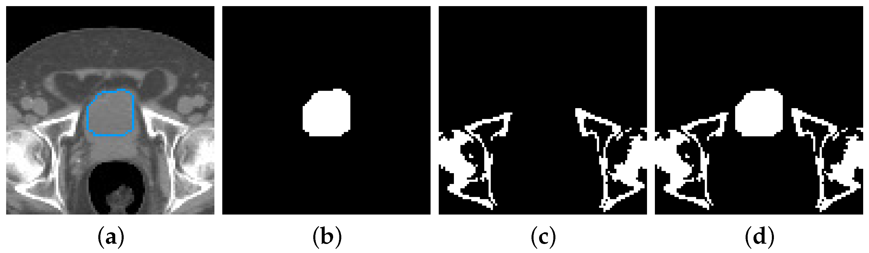
Figure 1. Image and structure set data from a single CT slice: (a) Delineation of a bladder (in blue) over the corresponding planning CT image (b) Bitmap representation of the bladder (c) Bony anatomy of the same CT, created with a density-based filter (d) Combination of the structure set and bony anatomy data.
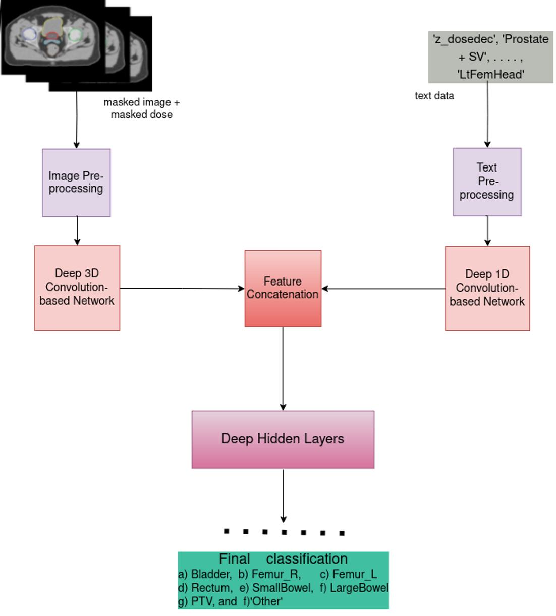
Biomedinformatics 03 00034 g001
Figure 2. Pictorial Representation of our Masking Step in the case of (a) images, and (b) doses of Prostate RT Patients.
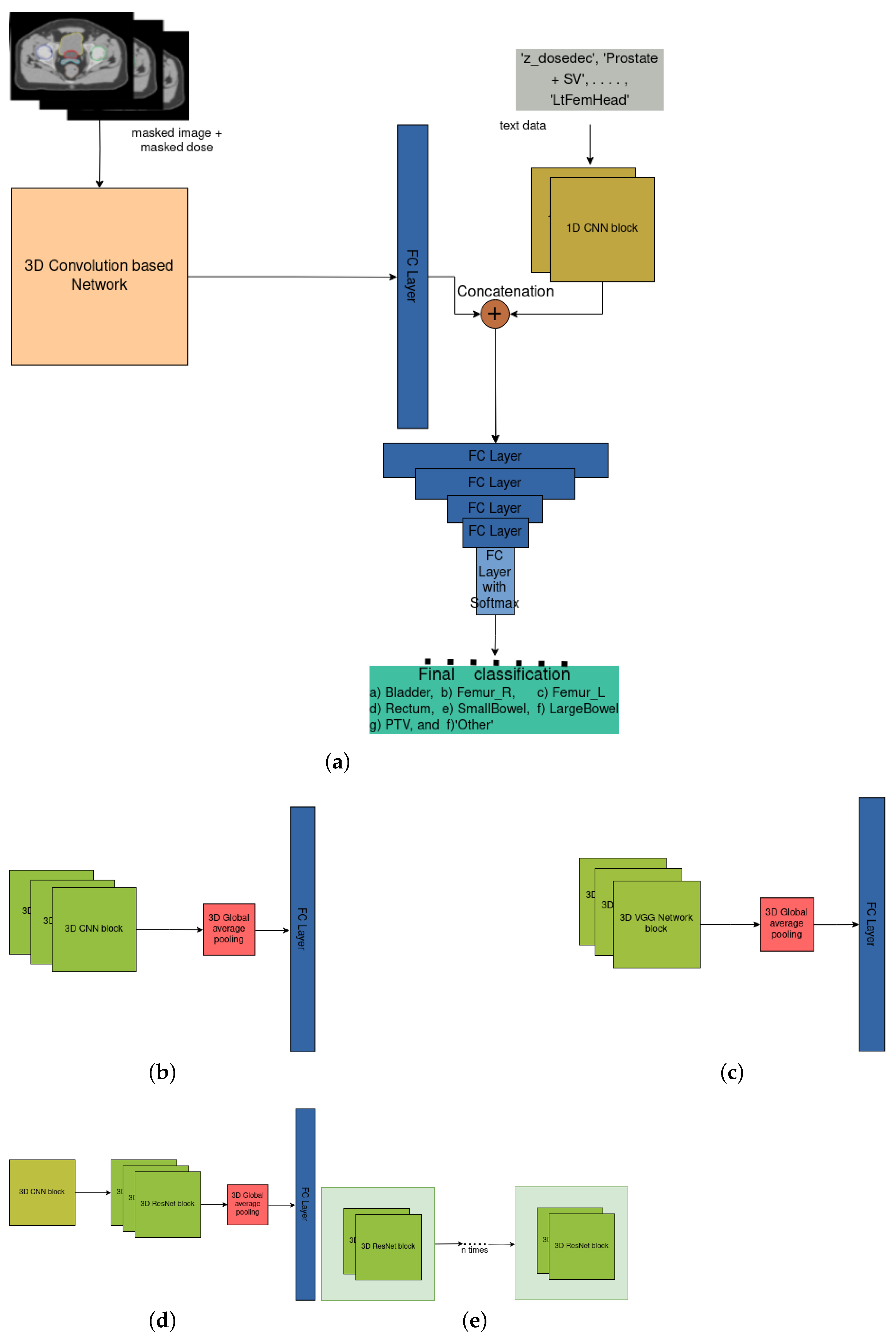
Biomedinformatics 03 00034 g002
Figure 3. Overview of our DNN architecture: (a) General architecture of our 3D Convolution-based network on vision-dose data and 1D CNN on text data, (b) Customized 3D CNN on vision-dose, (c) Customized 3D VGG network on vision-dose, (d) Customized 3D ResNet on vision-dose, (e) Stacked customized 3D VGG Network blocks with nested 3D ResNet blocks inside each block on vision-dose data.
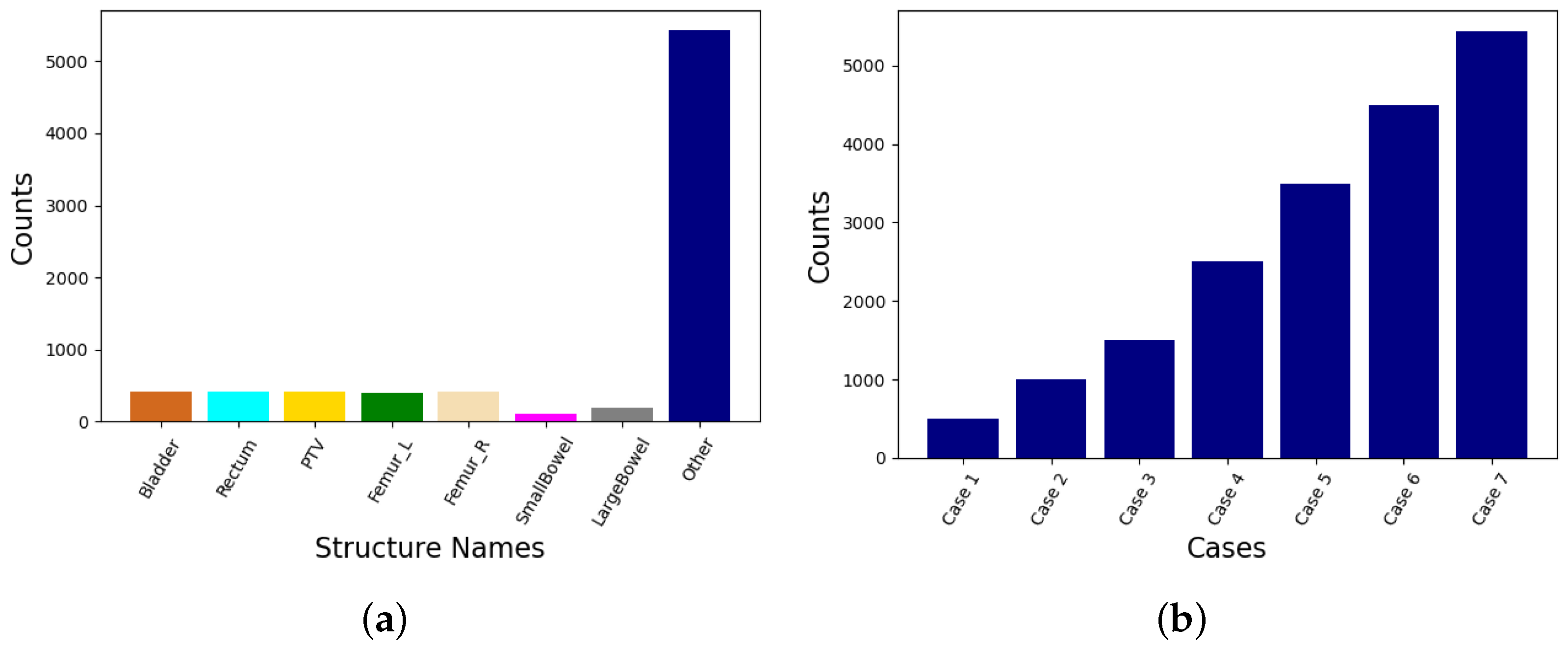
Biomedinformatics 03 00034 g003
Figure 4. Bar plots showing (a) the distribution of various data classes in the RT Prostate Structure Naming Dataset, and (b) the variation in the number of samples from the ‘Other’ class in different cases of consideration.
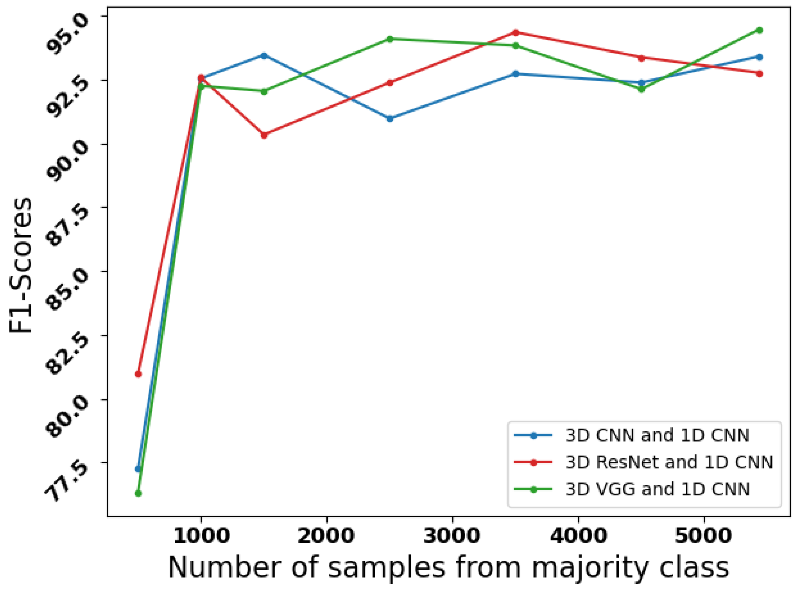
Biomedinformatics 03 00034 g004
Figure 5. Line curve showing the variation in F1-Scores of the model with variation in the number of samples from the majority ‘Other’ class.
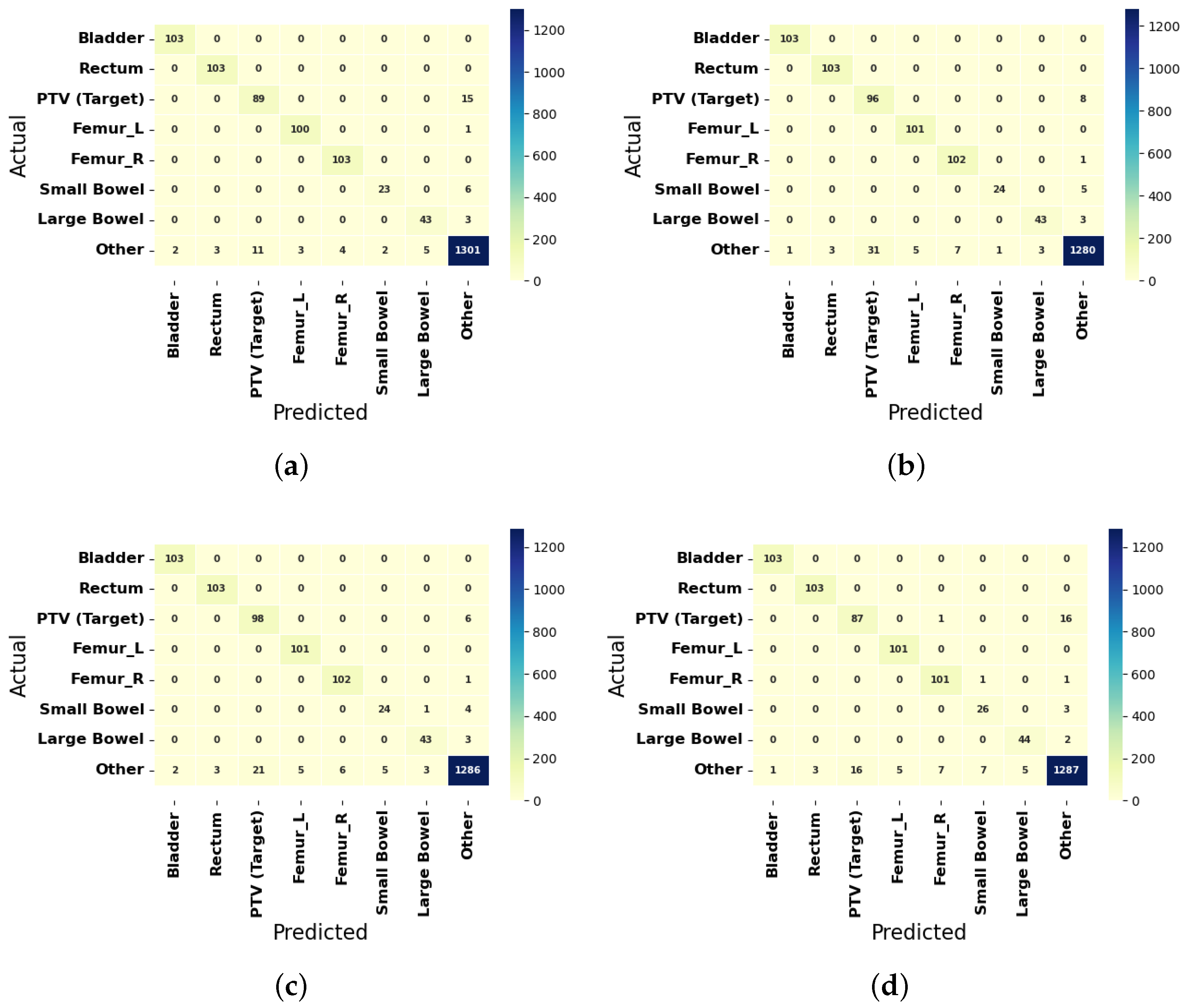
Biomedinformatics 03 00034 g005
Figure 6. Confusion Matrices of the best three predictions for the Prostate Cancer Patients by the F1-Scores are shown in (a) 3D VGG network and 1D CNN without undersampling, (b) 3D ResNet and 1D CNN with 3500 majority class samples, and (c) 3D VGG network and 1D CNN with 2500 majority class samples. Confusion Matrices of the best predictions of the architecture for the Prostate Cancer Patients by the F1-Scores are shown in (d) 3D CNN and 1D CNN with 1500 majority class samples.
Biomedinformatics 03 00034 g006
Table 1. Distribution of the Organ structure for the Prostate Cancer Patients.
Standard NamesVHA Physician Given Name CountsVCU Physician Given Name CountsTotal Physician Given Name CountsAvailable Given Name Counts
Bladder60950659519
Rectum71950769517
PTV (Target)71438752522
Femur_L69429723508
Femur_R70029729515
SmallBowel25049299145
LargeBowel3410341234
‘Other’11,03898012,0186763
Prostate Total15,065122516,2909723
Table 2. Distribution of the Physician Given Structure Names for the Prostate Cancer Patients.
Structure TypeStandard NamePatient 1Patient 2Patient 3
OARLargeBowelColon_Sigmoid--
OARFemur_RFemur_Head_RRtFemHeadHip Right
OARFemur_LFemur_Head_LLtFemHeadHip Left
OARBladderBladderbladderBladder
OARRectumRectumrectumRectum
OARSmallBowel-bowel-
TargetPTVPTV_7920PTV45GyPTV 2
‘Other’“Other”z post rectumptv4cmRectum − PTV
‘Other’“Other”BodynodalCTVfinalProstate + SV
‘Other’“Other”CTVpNONPTVBladPTV 1
‘Other’“Other”CouchInteriorCTVProsSVBladder − PTV
‘Other’“Other”PenileBulbExternalSeminal Vesicles
‘Other’“Other”ProstateFinalISOSeed Marker 1
‘Other’“Other”z_rectuminptvMarkedISODose 104 [%]
‘Other’“Other”z_dosedecCTVBstSeed Marker 3
Table 3. Performance of the CNN-based Models for the Prostate cancer patients during data selection.
Data ModalityMethodPrecision (in %)Recall (in %)F1-Score (in %)
struc+ image+ dose+ text3D CNN and 1D CNN91.9392.9392.42
struc+ image+ dose+ text3D ResNet and 1D CNN92.7293.7493.2
struc+ image+ dose+ text3D VGG and 1D CNN93.5192.9993.19
masked image+ masked dose+ text3D CNN and 1D CNN93.6593.2993.4
masked image+ masked dose+ text3D ResNet and 1D CNN91.0594.8392.76
masked image+ masked dose+ text3D VGG and 1D CNN94.6694.3994.45
Table 4. Model performances for the Prostate cancer patients with varying data modalities.
Masked ImageMasked DoseTextMethodPrecision (in %)Recall (in %)F1-Score (in %)
--3D CNN71.7574.8172.99
--3D ResNet73.9474.2473.92
--3D VGG76.1974.4674.82
--3D CNN74.1870.7972.17
--3D ResNet74.0162.9466.39
--3D VGG81.5377.9879.45
-3D CNN93.691.5291.93
-3D ResNet94.2393.6593.82
-3D VGG93.094.993.8
--1D CNN92.1894.2493.17
-3D CNN and 1D CNN93.3192.4992.83
-3D ResNet and 1D CNN91.3395.1893.15
-3D VGG and 1D CNN92.2491.3591.71
-3D CNN and 1D CNN91.8693.6692.61
-3D ResNet and 1D CNN90.1394.9792.29
-3D VGG and 1D CNN91.8293.4292.54
3D CNN and 1D CNN93.6593.2993.4
3D ResNet and 1D CNN91.0594.8392.76
3D VGG and 1D CNN94.6694.3994.45
Table 5. Model performances for the Prostate cancer patients with variation in the majority class samples.
Total Samples from ‘Other’ ClassMethodPrecision (in %)Recall (in %)F1-Score (in %)
5003D CNN and 1D CNN70.6289.3277.26
5003D ResNet and 1D CNN76.4787.2180.98
5003D VGG and 1D CNN71.7183.6176.33
10003D CNN and 1D CNN90.9994.2492.54
10003D ResNet and 1D CNN89.0896.9192.57
10003D VGG and 1D CNN89.8295.1692.25
15003D CNN and 1D CNN91.6595.4693.46
15003D ResNet and 1D CNN86.6395.390.34
15003D VGG and 1D CNN88.7996.3592.05
25003D CNN and 1D CNN87.8294.790.97
25003D ResNet and 1D CNN88.8696.792.38
25003D VGG and 1D CNN92.5695.7694.09
35003D CNN and 1D CNN91.7493.7592.72
35003D ResNet and 1D CNN93.695.4794.35
35003D VGG and 1D CNN92.4895.3693.83
45003D CNN and 1D CNN92.3492.5692.38
45003D ResNet and 1D CNN91.5495.4593.37
45003D VGG and 1D CNN91.4292.9592.12
5432 (No Sampling)3D CNN and 1D CNN93.6593.2993.4
5432 (No Sampling)3D ResNet and 1D CNN91.0594.8392.76
5432 (No Sampling)3D VGG and 1D CNN94.6694.3994.45
Table 6. Model performances with 3D VGG nested ResNet and 3D VGG with Leaky ReLU activation for the Prostate cancer patients while varying the majority class samples.
Total Samples from ‘Other’ ClassMethodPrecision (in %)Recall (in %)F1-Score (in %)
5003D VGG with nested ResNet and 1D CNN86.7596.3790.62
5003D VGG with LeakyReLU and 1D CNN85.5796.2889.74
10003D VGG with nested ResNet and 1D CNN87.3795.4990.92
10003D VGG with LeakyReLU and 1D CNN83.5697.2988.55
15003D VGG with nested ResNet and 1D CNN89.6796.2792.64
15003D VGG with LeakyReLU and 1D CNN91.6695.493.44
25003D VGG with nested ResNet and 1D CNN90.893.3892.02
25003D VGG with LeakyReLU and 1D CNN87.9296.2691.5
35003D VGG with nested ResNet and 1D CNN90.57 495.692.89
35003D VGG with LeakyReLU and 1D CNN88.5694.7591.44
45003D VGG with nested ResNet and 1D CNN90.9793.3392.11
45003D VGG with LeakyReLU and 1D CNN92.6992.3592.51
5432 (No Sampling)3D VGG with nested ResNet and 1D CNN92.1994.7193.36
5432 (No Sampling)3D VGG with LeakyReLU and 1D CNN91.9594.2993.04
Table 7. Class-wise performances of the top three Models for the Prostate cancer patients.
ClassVGG (with 5432 Majority Class Samples)ResNet (3500 Majority Class Samples)VGG (2500 Majority Class Samples)
Precision (in %)Recall (in %)F1-Score (in %)Precision (in %)Recall (in %)F1-Score (in %)Precision (in %)Recall (in %)F1-Score (in %)
Bladder98.110099.0499.0410099.5298.110099.04
Rectum97.1710098.5697.1710098.5697.1710098.56
PTV (Target)89.085.5887.2575.5992.3183.1282.3594.2387.89
Femur_L97.0999.0198.0495.2810097.5895.2810097.58
Femur_R96.2610098.193.5899.0396.2394.4499.0396.68
Small Bowel92.079.3185.1996.082.7688.8982.7682.7682.76
Large Bowel89.5893.4891.4993.4893.4893.4891.4993.4892.47
‘Other’98.1197.7597.9398.6996.1797.4198.9296.6297.76
Disclaimer/Publisher’s Note: The statements, opinions and data contained in all publications are solely those of the individual author(s) and contributor(s) and not of MDPI and/or the editor(s). MDPI and/or the editor(s) disclaim responsibility for any injury to people or property resulting from any ideas, methods, instructions or products referred to in the content.

