
Detection of Myocardial Infarction Using Hybrid Models of Convolutional Neural Network and Recurrent Neural Network

Abstract
:
1. Introduction
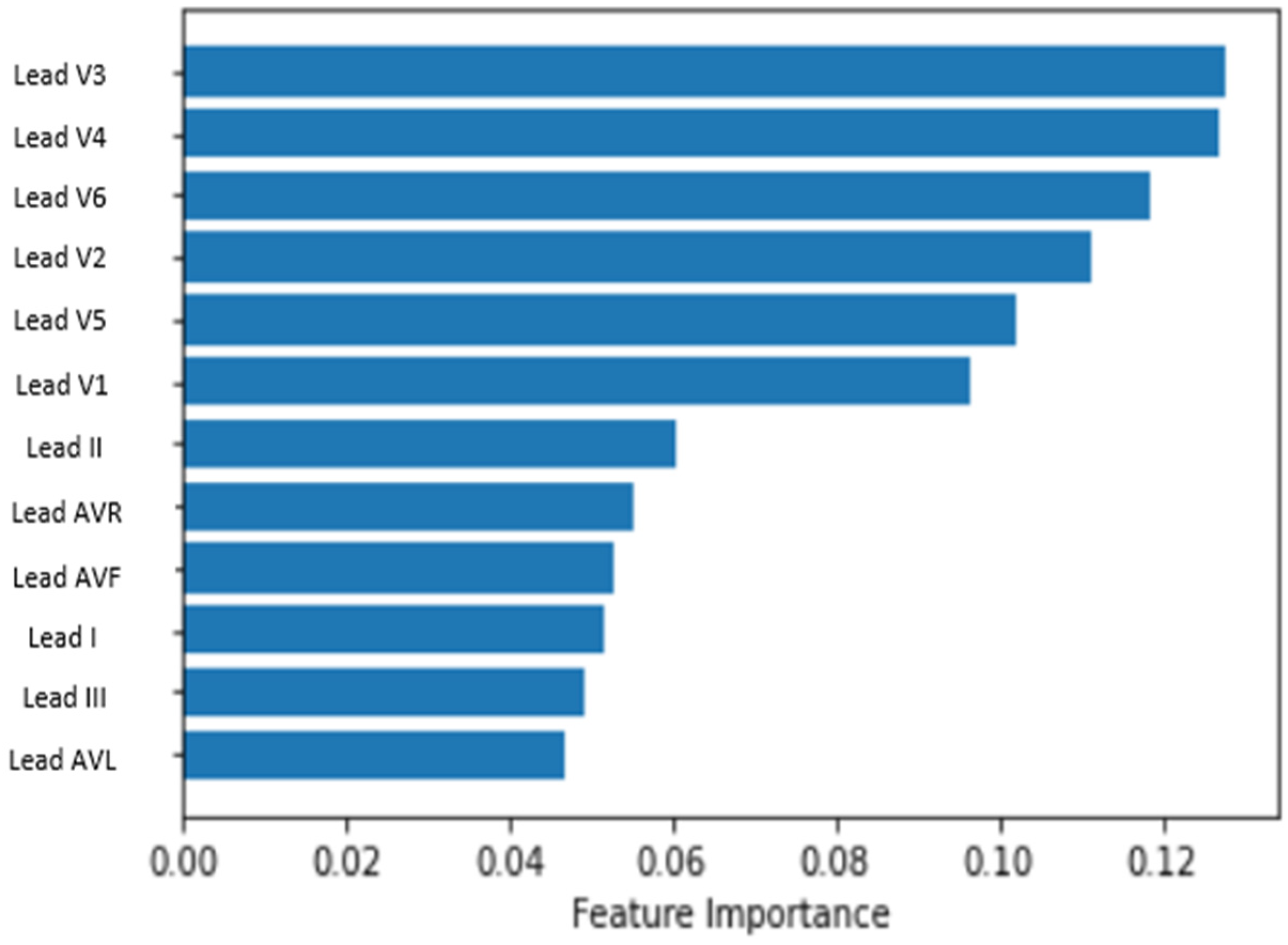
- Identification of most relevant leads for MI detection from the PTB XL dataset for efficient use of computational resources in model development and training.
- Proposed models with straightforward architecture that better use the inherent capabilities of CNN and LSTM/BILSTM.
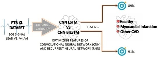
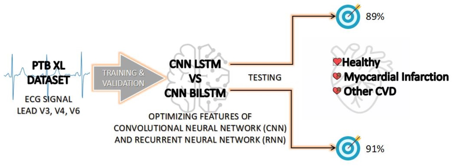
- Development of CNN LSTM and CNN BILSTM models to predict MI with three outputs: MI, Healthy and Other CVD.
2. Related Works
3. Materials and Methods
3.1. Dataset
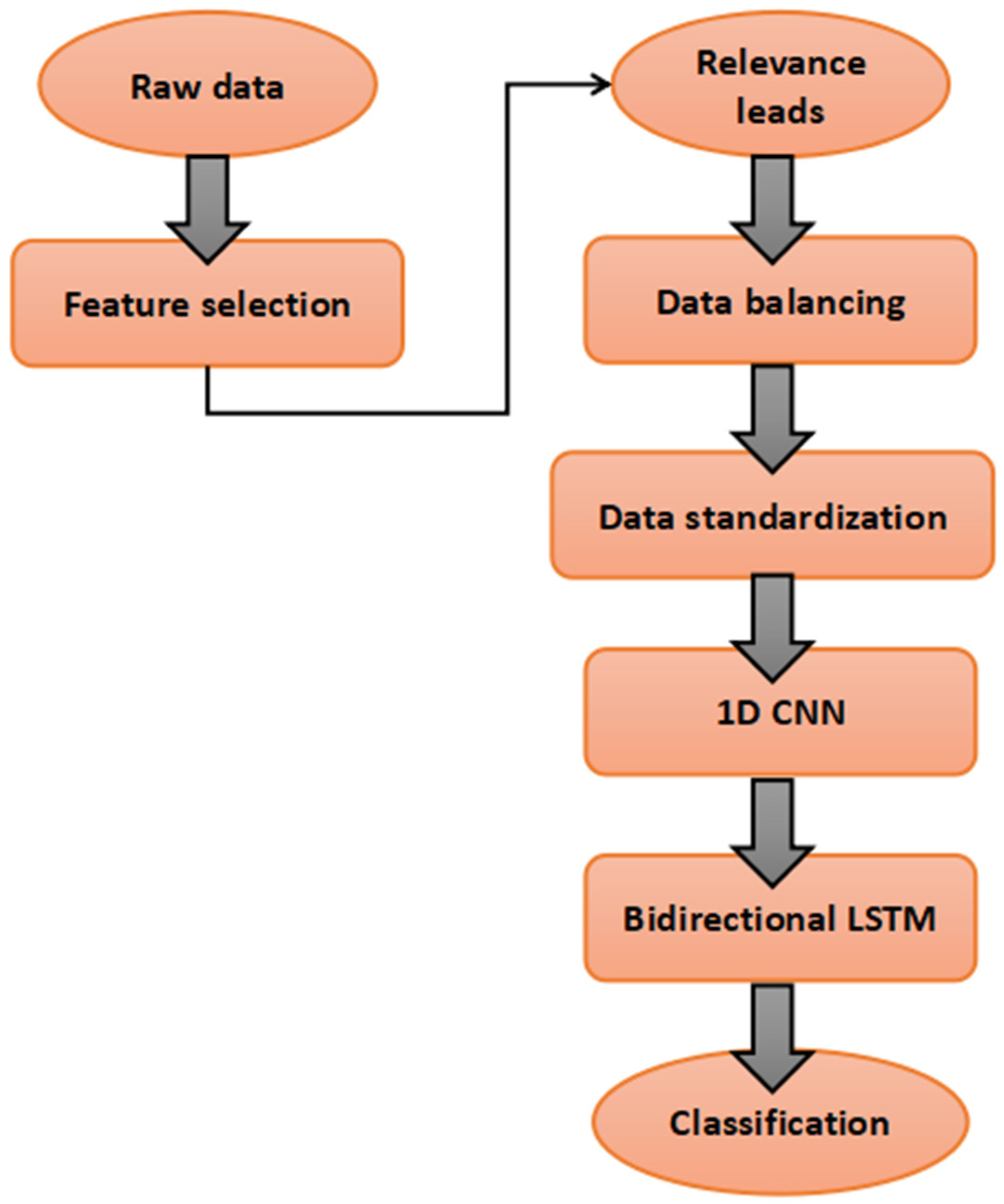
3.2. Data Cleaning and Selection of ECG Lead
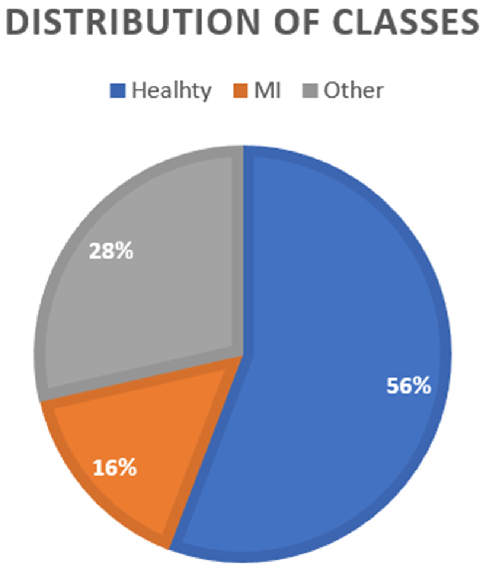
3.3. Data Balancing
3.4. Proposed Model
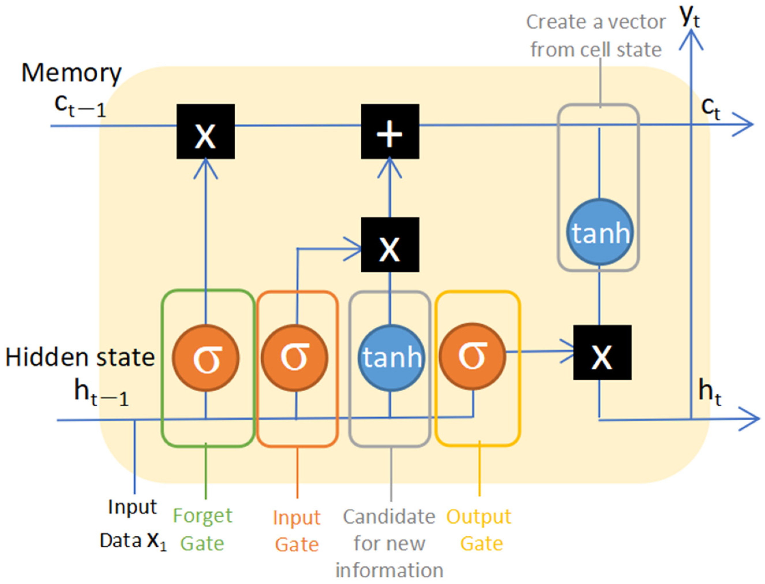
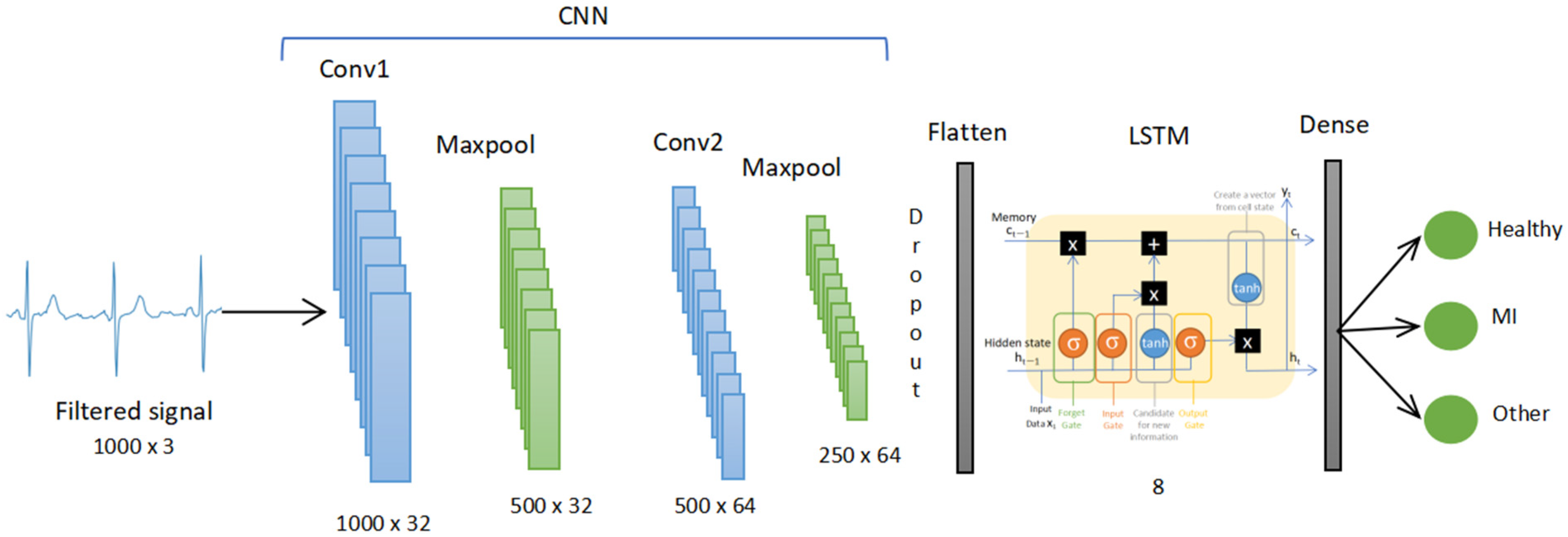
3.4.1. CNN LSTM
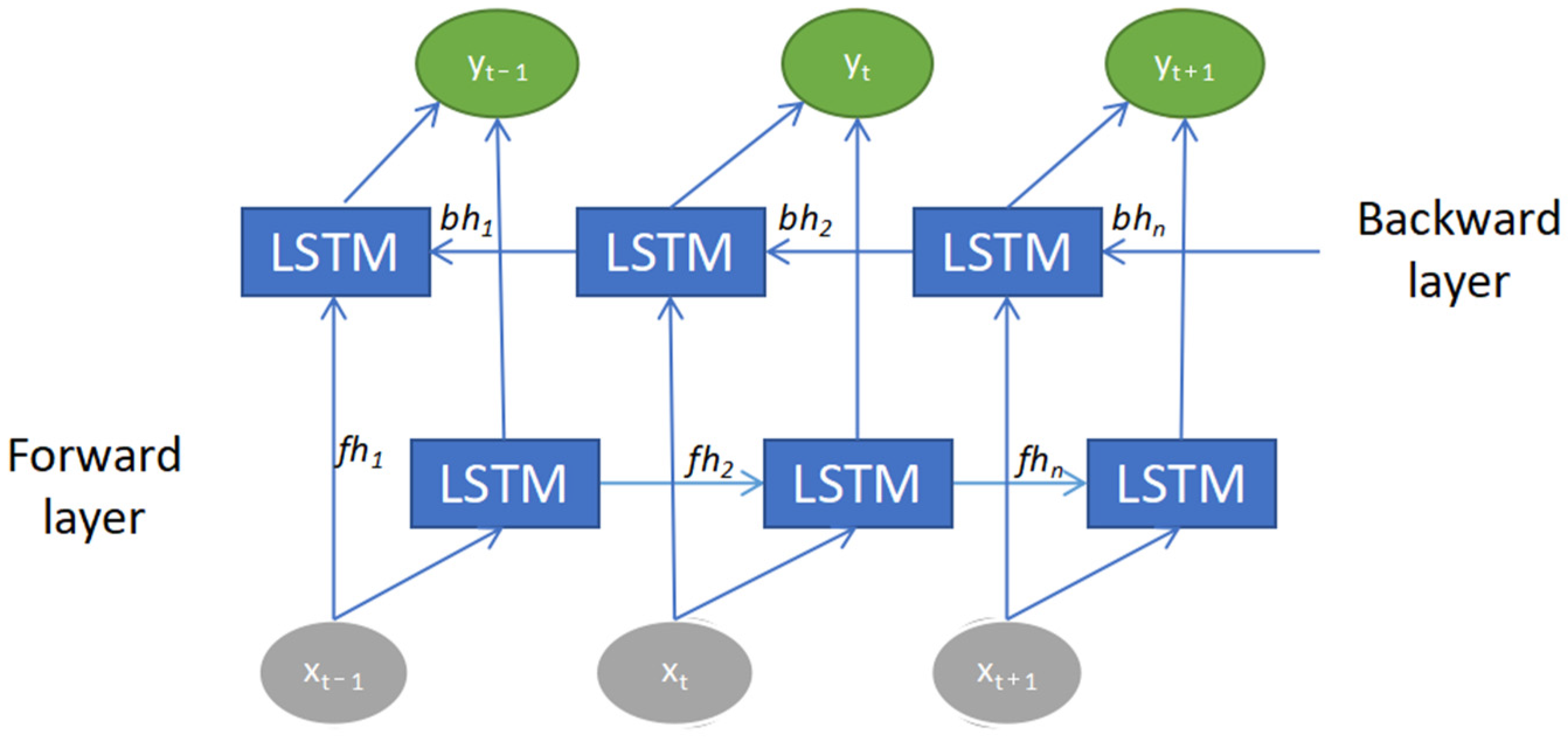
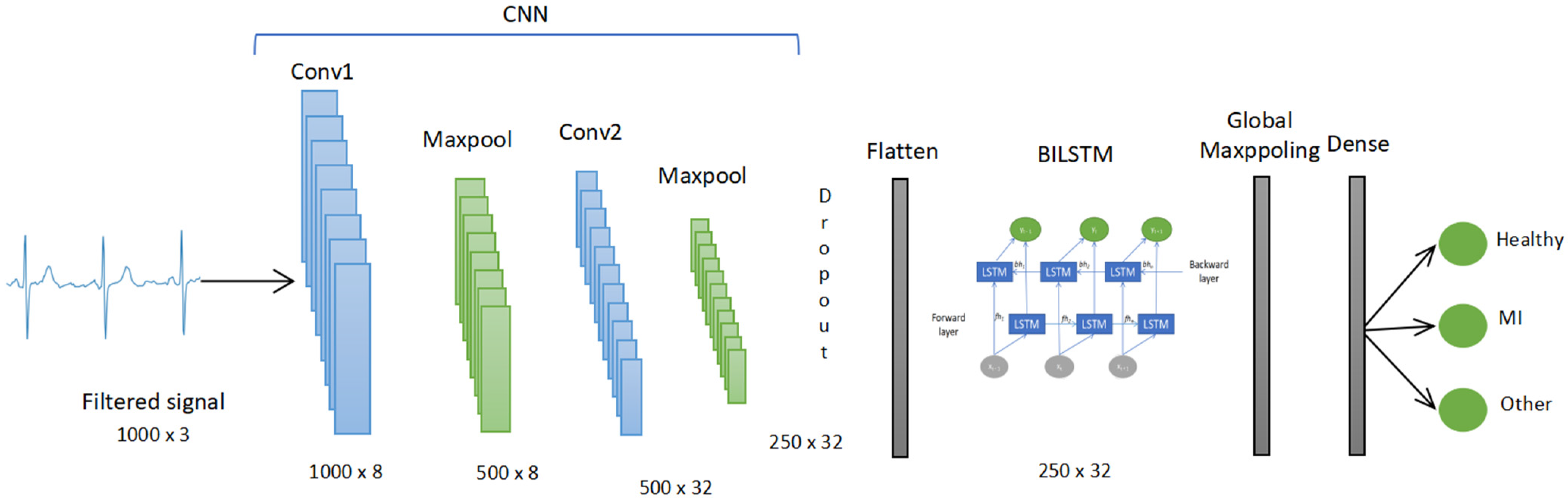
3.4.2. CNN BILSTM
3.5. Evaluation Metrics
4. Results
4.1. Selection of ECG Leads
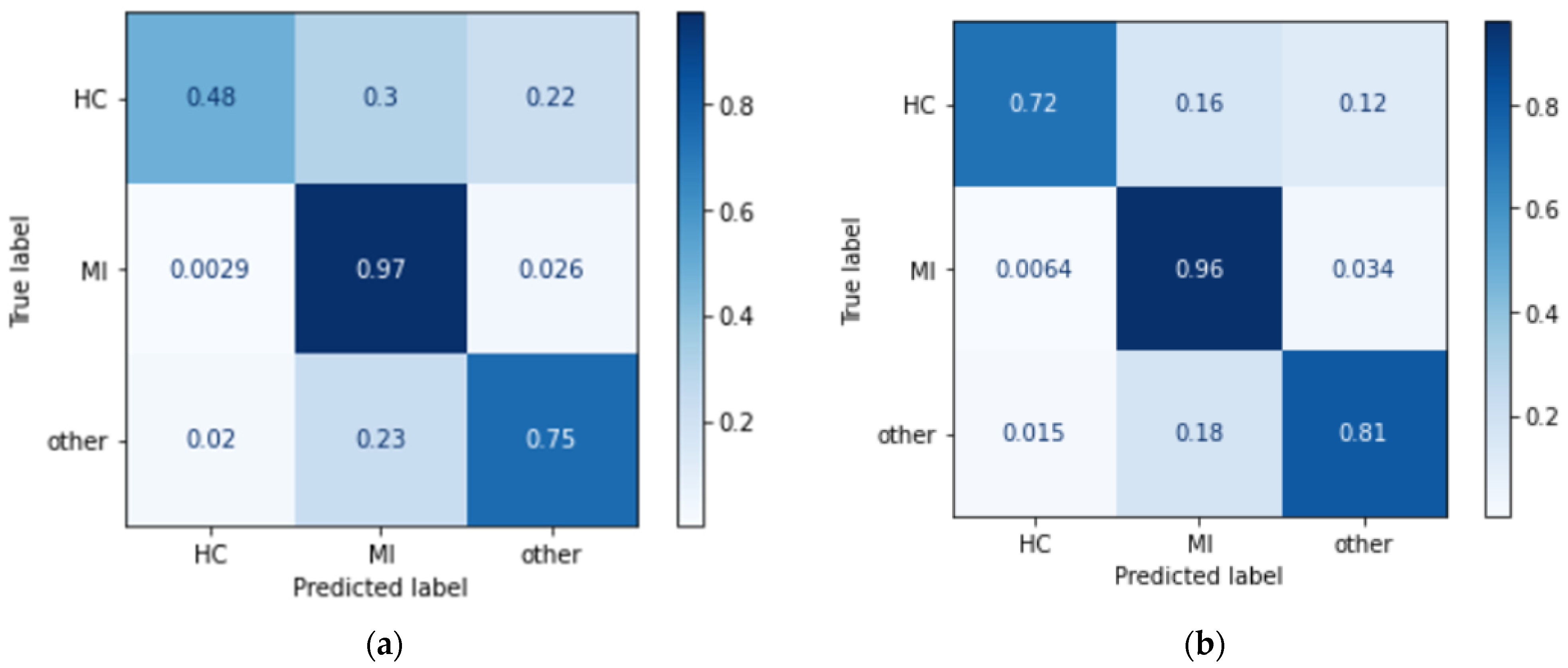
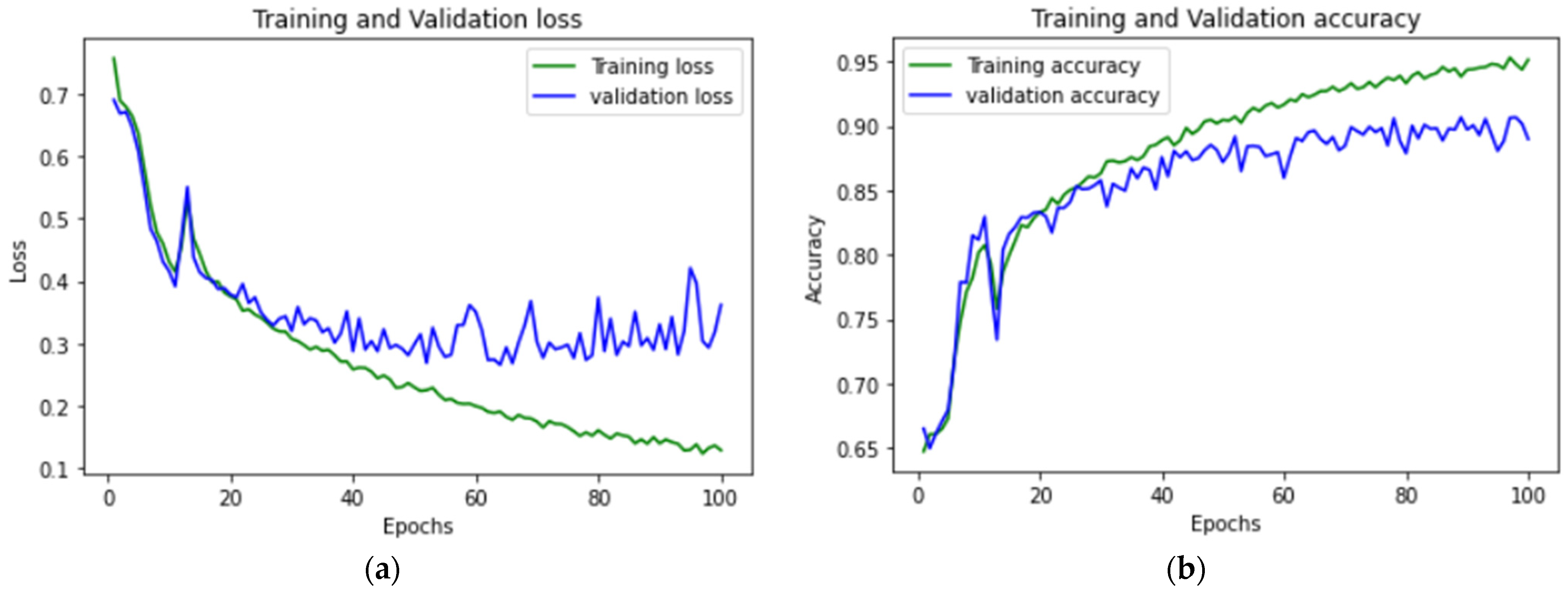
4.2. Model Performance
5. Discussion
6. Conclusions
Author Contributions
Funding
Data Availability Statement
Conflicts of Interest
References
- Cardiovascular Diseases. Available online: https://www.who.int/health-topics/cardiovascular-diseases#tab=tab_1 (accessed on 4 January 2023).
- Electrocardiogram (ECG or EKG). Available online: https://www.heart.org/en/health-topics/heart-attack/diagnosing-a-heart-attack/electrocardiogram-ecg-or-ekg (accessed on 4 January 2023).
- Learning the PQRST EKG Wave Tracing. Available online: https://www.registerednursern.com/learning-the-pqrst-ekg-wave-tracing/ (accessed on 4 January 2023).
- PR Interval. Available online: https://litfl.com/pr-interval-ecg-library/ (accessed on 4 January 2023).
- Sun, L.; Lu, Y.; Yang, K.; Li, S. ECG Analysis Using Multiple Instance Learning for Myocardial Infarction Detection. IEEE Trans. Biomed. Eng. 2012, 59, 3348–3356. [Google Scholar] [CrossRef] [PubMed]
- Chumachenko, D.; Butkevych, M.; Lode, D.; Frohme, M.; Schmailzl, K.J.; Nechyporenk, A. Machine Learning Methods in Predicting Patients with Suspected Myocardial Infarction Based on Short-Time HRV Data. Sensors 2022, 22, 7033. [Google Scholar] [CrossRef] [PubMed]
- Dhawan, A.; Briain, W.; George, S.; Gussak, I.; Bojovic, B.; Panescu, D. Detection of acute myocardial infarction from serial ECG using multilayer support vector machine. In Proceedings of the 2012 Annual International Conference of the IEEE Engineering in Medicine and Biology Society, San Diego, CA, USA, 28 August–1 September 2012. [Google Scholar]
- Dohare, A.K.; Kumar, V.; Kumar, R. Detection of myocardial infarction in 12 lead ECG using support Vector Machine. Appl. Soft Comput. 2018, 64, 138. [Google Scholar] [CrossRef]
- Thatipelli, T.; Kora. P. Classification of Myocardial Infarction using Discrete Wavelet. Int. Res. J. Eng. Technol. (IRJET) 2017, 4, 429–432. [Google Scholar]
- Zhang, X.; Li, R.; Dai, H.; Liu, Y.; Zhou, B.; Wang, Z. Localization of myocardial infarction with multi-lead bidirectional gated recurrent unit neural network. IEEE Access 2019, 7, 161152–161166. [Google Scholar] [CrossRef]
- Deep Learning, vs. Machine Learning: Beginner’s Guide. Available online: https://www.coursera.org/articles/ai-vs-deep-learning-vs-machine-learning-beginners-guide (accessed on 10 February 2023).
- Kagiyama, N.; Shrestha, S.; Farjo, P.D.; Sengupta, P.P. Artificial Intelligence: Practical Primer for Clinical Research in Cardiovascular Disease. J. Am. Heart Assoc. 2019, 8, e012788. [Google Scholar] [CrossRef]
- Mirza, A.H.; Nurmaini, S.; Partan, R.U. Automatic classification of 15 leads ECG signal of myocardial infarction using one dimension convolutional neural network. Appl. Sci. 2022, 12, 5603. [Google Scholar] [CrossRef]
- Choudhary, P.S.; Dandapat, S. Multibranch 1D CNN for detection and localization of myocardial infarction from 12 lead electrocardiogram signal. In Proceedings of the 2021 IEEE 18th India Council International Conference (INDICON), Guwahati, India, 19–21 December 2021. [Google Scholar]
- Rajendra, U.A.; Fujita, H.; Oh, S.L.; Hagiwara, Y.; Tan, J.H.; Adam, M. Application of deep convolutional neural network for automated detection of myocardial infarction using ECG signals. Inf. Sci. 2017, 415–416, 190–198. [Google Scholar]
- Ibrahim, L.; Mesinovic, M.; Yang, K.W.; Eid, M.A. Explainable prediction of acute myocardial infarction using machine learning and Shapley Values. IEEE Access 2020, 8, 210410–210417. [Google Scholar] [CrossRef]
- Li, W.; Tang, Y.M.; Yu, K.M.; To, S. SLC-gan: An automated myocardial infarction detection model based on generative adversarial networks and convolutional neural networks with single-lead electrocardiogram synthesis. Inf. Sci. 2022, 589, 738–750. [Google Scholar] [CrossRef]
- Zhang, X.; Li, R.; Hu, Q.; Zhou, B.; Wang, Z. A new automatic approach to distinguish myocardial infarction based on LSTM. In Proceedings of the 2019 8th International Symposium on Next Generation Electronics (ISNE), Zhengzhou, China, 9–10 October 2019. [Google Scholar]
- Martin, H.; Morar, U.; Izquierdo, W.; Cabrera, A.; Adjouadi, M. Real-time frequency-independent single-lead and single-beat myocardial infarction detection. Artif. Intell. Med. 2021, 121, 102179. [Google Scholar] [CrossRef] [PubMed]
- Lui, H.W.; Chow, K.L. Multiclass classification of myocardial infarction with convolutional and recurrent neural networks for portable ECG devices. Inform. Med. Unlocked 2018, 13, 26–33. [Google Scholar] [CrossRef]
- Feng, K.; Pi, X.; Liu, H.; Sun, K. Myocardial infarction classification based on Convolutional Neural Network and recurrent neural network. Appl. Sci. 2019, 9, 1879. [Google Scholar] [CrossRef] [Green Version]
- Wu, L.; Huang, G.; Yu, X.; Ye, M.; Liu, L.; Ling, Y.; Liu, X.; Liu, D.; Zhou, B.; Liu, Y.; et al. Deep Learning Networks accurately detect st-segment elevation myocardial infarction and culprit vessel. Front. Cardiovasc. Med. 2022, 9, 797207. [Google Scholar] [CrossRef] [PubMed]
- Liu, W.; Wang, F.; Huang, Q.; Chang, S.; Wang, H.; He, J. MFB-CBRNN: A hybrid network for MI detection using 12-lead ecgs. IEEE J. Biomed. Health Inform. 2020, 24, 503–514. [Google Scholar] [CrossRef] [PubMed]
- Dey, M.; Omar, N.; Ullah, M.A. Temporal Feature-Based Classification Into Myocardial Infarction and Other CVDs Merging CNN and Bi-LSTM From ECG Signal. IEEE Sens. J. 2021, 21, 21688–21695. [Google Scholar] [CrossRef]
- Wagner, P.; Strodthoff, N.; Bousseljot, R.D.; Kreiseler, D.; Lunze, F.I.; Samek, W.; Schaeffter, T. PTB-XL, a large publicly available electrocardiography dataset. Sci. Data 2020, 7, 154. [Google Scholar] [CrossRef]
- Kumar, V.; Lalotra, G.S.; Sasikala, P.; Rajput, D.S.; Kaluri, R.; Lakshmanna, K.; Shorfuzzaman, M.; Alsufyani, A.; Uddin, M. Addressing Binary Classification over Class Imbalanced Clinical Datasets Using Computationally Intelligent Techniques. Healthcare 2022, 10, 1293. [Google Scholar] [CrossRef]
- Gogul, I.; Kumar, V.S. Flower species recognition system using convolution neural networks and transfer learning. In Proceedings of the 2017 Fourth International Conference on Signal Processing, Communication and Networking (ICSCN), Chennai, India, 16–18 March 2017. [Google Scholar]
- Part of Course 321 One Dimensional Convolutional Neural Networks. Available online: https://e2eml.school/convolution_one_d.html (accessed on 10 April 2023).
- Long Short Term Memory: Architecture of LSTM. Available online: https://www.analyticsvidhya.com/blog/2017/12/fundamentals-of-deep-learning-introduction-to-lstm (accessed on 13 February 2023).
- How to Develop a Bidirectional LSTM for Sequence Classification in Python with Keras. Available online: https://machinelearningmastery.com/develop-bidirectional-lstm-sequence-classification-python-keras (accessed on 13 February 2023).
- Shyamalee, T.; Meedeniya, D. Glaucoma Detection with Retinal Fundus Images Using Segmentation and Classification. Mach. Intell. Res. 2022, 19, 563–580. [Google Scholar] [CrossRef]
- Maturo, F.; Verde, R. Pooling Random Forest and functional data analysis for biomedical signals supervised classification: Theory and application to Electrocardiogram Data. Stat. Med. 2022, 41, 2247–2275. [Google Scholar] [CrossRef]
- Sabri, M.; Maturo, F.; Verde, R.; Riffi, J.; Yahyaouy, A. Classification of ECG signals based on functional data analysis and machine learning techniques. In Proceedings of the Conference: IES 2022—Innovation and Society 5.0: Statistical and Economic Methodologies for Quality Assessment, Capua, Italy, 27–28 January 2022. [Google Scholar]
- Pfisterer, F.; Beggel, L.; Sun, X.; Scheipl, F.; Bischl, B. Benchmarking time series classification—Functional data vs. machine learning approaches. arXiv 2019, arXiv:1911.07511. [Google Scholar]


| Layer Type | Output Shape | Parameter |
|---|---|---|
| Conv1d-1 | 1000,32 | 992 |
| Activation_1 | 1000,32 | 0 |
| Batch_normalization_1 | 1000,32 | 128 |
| Max_pooling1d_1 | 500,32 | 0 |
| Conv1d_2 | 500,64 | 20,544 |
| Activation_2 | 500,64 | 0 |
| Batch_normalization_2 | 500,32 | 256 |
| Max_pooling1d_2 | 250,64 | 0 |
| Dropout_1 | 250,64 | 0 |
| Time_distributed_1 | 250,64 | 0 |
| LSTM | 8 | 2336 |
| Dense_1 | 3 | 27 |
| Total params: 24,283 | ||
| Trainable params: 24,091 | ||
| Non-trainable params: 192 |
| Layer Type | Output Shape | Parameter |
|---|---|---|
| Conv1d-1 | 1000,8 | 248 |
| Activation_1 | 1000,8 | 0 |
| Batch_normalization_1 | 1000,8 | 32 |
| Max_pooling1d_1 | 500,8 | 0 |
| Conv1d_2 | 500,32 | 2592 |
| Activation_2 | 500,32 | 0 |
| Batch_normalization_2 | 500,32 | 128 |
| Max_pooling1d_2 | 250,32 | 0 |
| Dropout_1 | 250,32 | 0 |
| Time_distributed_1 | 250,32 | 0 |
| Bidirectional_1 | 250,32 | 6272 |
| Global_max_pooling1d_1 | 32 | 0 |
| Dense_1 | 3 | 99 |
| Total params: 9371 | ||
| Trainable params: 9291 | ||
| Non-trainable params: 80 |
| Performance Parameter | CNN LSTM Testing Result | CNN BILSTM Testing Result |
|---|---|---|
| Accuracy | 89% | 91% |
| Recall | Healthy: 48% | Healthy: 72% |
| MI: 97% | MI: 96% | |
| Other: 75% | Other: 81% | |
| Precision | Healthy: 52% | Healthy: 60% |
| MI: 89% | MI: 91% | |
| Other: 92% | Other: 91% | |
| F1-score | Healthy: 50% | Healthy: 65% |
| MI: 93% | MI: 93% | |
| Other: 83% | Other: 86% |
| No | Study | Architecture | Dataset | Additional Process | ECG Leads Used | Denoising | F1-Score |
|---|---|---|---|---|---|---|---|
| 1 | Hin Wan Lui et al. [20] | CNN | PTB and AF Challenge | - | Lead I | Yes | 59.70% |
| 2 | Hin Wan Lui et al. [20] | CNN with stacking decoding | PTB and AF Challenge | Stacking decoding | Lead I | Yes | 75.90% |
| 3 | Hin Wan Lui et al. [20] | CNN-LSTM | PTB and AF Challenge | - | Lead I | Yes | 73.00% |
| 4 | Hin Wan Lui et al. [20] | CNN-LSTM with stacking decoding | PTB and AF Challenge | Stacking decoding | Lead I | Yes | 94.60% |
| 5 | Monisha Dey et al. [24] | CNN-BILSTM | PTB | Manual feature extraction | 12 leads | Yes | 99.52% |
| 6 | Proposed model | CNN-BILSTM | PTB XL | - | Lead V3, V4 V6 | No | 93% |
Disclaimer/Publisher’s Note: The statements, opinions and data contained in all publications are solely those of the individual author(s) and contributor(s) and not of MDPI and/or the editor(s). MDPI and/or the editor(s) disclaim responsibility for any injury to people or property resulting from any ideas, methods, instructions or products referred to in the content. |
© 2023 by the authors. Licensee MDPI, Basel, Switzerland. This article is an open access article distributed under the terms and conditions of the Creative Commons Attribution (CC BY) license (https://creativecommons.org/licenses/by/4.0/).
Share and Cite
Hasbullah, S.; Mohd Zahid, M.S.; Mandala, S. Detection of Myocardial Infarction Using Hybrid Models of Convolutional Neural Network and Recurrent Neural Network. BioMedInformatics 2023, 3, 478-492. https://doi.org/10.3390/biomedinformatics3020033
Hasbullah S, Mohd Zahid MS, Mandala S. Detection of Myocardial Infarction Using Hybrid Models of Convolutional Neural Network and Recurrent Neural Network. BioMedInformatics. 2023; 3(2):478-492. https://doi.org/10.3390/biomedinformatics3020033
Chicago/Turabian StyleHasbullah, Sumayyah, Mohd Soperi Mohd Zahid, and Satria Mandala. 2023. "Detection of Myocardial Infarction Using Hybrid Models of Convolutional Neural Network and Recurrent Neural Network" BioMedInformatics 3, no. 2: 478-492. https://doi.org/10.3390/biomedinformatics3020033