Article

Beyond the Tide: A Comprehensive Guide to Sea-Level-Rise Inundation Mapping Using FOSS4G

1
GIS Center, Florida International University, Miami, FL 33199, USA
2
Institute of Environment, Florida International University, Miami, FL 33199, USA
*
Author to whom correspondence should be addressed.
Geomatics 2023, 3(4), 522-540; https://doi.org/10.3390/geomatics3040028
Submission received: 4 November 2023 / Revised: 22 November 2023 / Accepted: 23 November 2023 / Published: 28 November 2023
(This article belongs to the Special Issue GIS Open Source Software Applied to Geosciences)

Abstract

:
Sea-level rise (SLR) is a critical consequence of climate change, posing significant threats to coastal regions worldwide. Accurate and efficient assessment of potential inundation areas is crucial for effective coastal planning and adaptation strategies. This study aimed to explore the utility of free and open-source software for geospatial (FOSS4G) tools for mapping SLR inundation, providing cost-effective solutions that are accessible to researchers and policymakers. We employed a combination of geospatial data, including high-resolution elevation models, tidal data, and projected SLR scenarios. Utilizing widely available FOSS4G tools, like QGIS, GDAL/OGR, and GRASS GIS, we developed an integrated workflow to map inundation extents, using a passive bathtub approach for various SLR scenarios. We demonstrate the approach through a case study in Virginia Key, Florida, however, the methodology can be replicated in any area where the input datasets are available. This paper demonstrates that FOSS4G tools offer a reliable and accessible means to map SLR inundation, empowering stakeholders to assess coastal vulnerabilities and to devise sustainable adaptation measures. The open-source approach facilitates collaboration and reproducibility, fostering a comprehensive understanding of the potential impacts of SLR on coastal ecosystems and communities.

1. Introduction

Climate change has become a severe issue for the planet, with an increase in the average global temperature leading to more frequent and severe weather events [1,2]. This rise in temperature causes ice sheets and glaciers to melt, contributing to sea-level rise (SLR) [3]. With record-breaking temperatures this year in southern states in the United States (e.g., Nevada, Arizona, Texas, and Florida [4,5]), coupled with the trend of increasing ocean temperature and the unprecedented melting speed of ice, an inevitable sea-level rise is occurring. Even small increases in sea levels pose heightened risk when combined with king tides and storm surges, especially considering that approximately 400 million people live within 20 m of sea level and within 20 km of the coastline worldwide [6]. Sea-level rise could result in a series of consequences, such as saltwater intrusion into inland rivers contaminating freshwater resources and harming agricultural lands [7,8]. Coastal ecosystems—like mangroves, marshes, and coral reefs—can be altered, resulting in the loss of habitats for certain species [9,10]. For human communities, shoreline infrastructure and properties are vulnerable to flooding, and homeowners may be forced to relocate, significantly disrupting the local economy [11]. Thus, to cope with the impact of sea-level rise and to prepare for future climate change, it is crucial to map the inundation in different sea-level-rise scenarios. This paper presents an alternative to propriatery software approaches to achieve this.
The remainder of the paper is structured as follows. Section 1.1 gives an overview of the related literature, while Section 1.2 explains the novelty of our contribution. Section 2 describes the datasets and algorithms necessary for mapping SLR. More specifically, Section 2.1 discusses elevation and water surface datasets and related vertical reference systems, while Section 2.2 explains the mapping process. Our FOSS4G (free and open-source software for geospatial) implementation is described in Section 2.3, followed by the description of a case study in Section 2.4. The results of a case study demonstrating the approach are presented in Section 3, and finally, Section 4 concludes the work and places it in context.

1.1. Previous Work

Currently, various models are used in SLR inundation modeling. Based on the different spatial scales, complexity of computation, and data involved in the models, SLR models can be generally divided into hydrodynamic models and GIS-based approaches [12]. Hydrodynamic models—such as the SLOSH (Sea, Lake, and Overland Surges from Hurricanes) model tailored to specific shoreline intricacies [13], Delft3D focusing on hydrodynamics and sediment transport [14], and ADCIRC (Advance Circulation Model for Coastal Ocean Hydrodynamics) modeling coastal water levels and currents—aim to replicate the dynamics of water inundation [15]. Although they are effective for predicting hurricane-driven storm surges, these models are constrained to specific areas, due to their intricate demands for expertise, data, and computational power. By contrast, GIS-based models are emerging as a more accessible method to map SLR inundation. Requiring decent data quality and computational resources, they are also easily adaptable to various regions [16]. Medium-resolution GIS techniques sufficiently address the needs of scientific research, coastal management, and spatial planning in understanding coastal processes and assessing hazards [12]. Prominent GIS-based models include SLAMM (Sea-Level-Affecting-Marshes Model), which relies on elevation data, BTELSS (Barataria–Terrebonne-Ecological-Landscape Spatial Simulation) addressing regional coastal dynamics [17,18], and the widely used Bathtub model [19,20]. Williams and Lück-Vogel [12]’s enhanced version of the Bathtub model offers improved accuracy in storm surge contexts by considering additional parameters. Some GIS models, like DIVA, even delve into the broader impacts of SLR, including socioeconomic and biophysical implications, as well as the adaptive strategies’ costs and benefits [21,22]. The web applications NOAA (National Oceanic and Atmospheric Administration)’s Sea-Level-Rise Viewer (https://coast.noaa.gov/digitalcoast/tools/slr.html, accessed on 3 November 2023) and Climate Central’s Coastal-Risk Screening Tool (https://coastal.climatecentral.org/, accessed on 3 November 2023) are just two examples that popularize SLR inundation mapping by making SLR-scenario maps available to the public.
While multiple examples of flood-related FOSS4G solutions exist [23,24,25], most models and studies rely on proprietary software. For example, Lichter and Felsenstein [26] crafted an automated method utilizing ArcGIS geo-processing commands in Python to locally gauge the financial implications of SLR and intense flooding. Li et al. [27] and Perini et al. [28] both developed their coastal inundation models with the aid of ESRI’s cost-distance tool, while both models take into account hydrological connectivity to the coastline, and the latter also factors in the beach slope that sea-borne inundation water must traverse. Additionally, NOAA’s popular SLR Viewer tool employs ArcGIS software for SLR inundation mapping [29]. While the capabilities of proprietary software are undeniably useful for modeling SLR scenarios, their proprietary nature limits broader adoption and utilization.
With the advancement of the open-data policy issued by the Office of Management and Budget (OMB) in 2013, accessibility to geospatial data has significantly improved [30]. In the context of U.S. policy, the Federal Geographic Data Committee (FGDC), founded in 1990, aims to promote the coordinated development, utilization, sharing, and dissemination of geospatial data across all governmental levels, the private sector, non-profit entities, and academic institutions [31]. In 2001, the geospatial one-stop initiative introduced a portal for the discovery and retrieval of geospatial assets from various governmental bodies, and it has been embraced by professionals, from urban planners and researchers to policymakers, all of whom depend on spatial data for informed decision making [32]. The Geospatial Data Act of 2018 further emphasized the importance of public accessibility, endorsing data sharing across governmental tiers, all while heeding privacy and security concerns [33]. This Act has underscored the principles of collaboration, transparency, and efficiency in geospatial data usage. With the progress made in open-data policies, the development of free and open-source software (FOSS) has also kept pace. The adoption of FOSS offers several advantages, including cost reduction, vendor independence, heightened customizability, assured interoperability, and robust community support. There has been a notable momentum in the geospatial domain towards such open-source paradigms, namely free and open-source software for geospatial (FOSS4G). FOSS4G’s value, particularly in an economic context, has been highlighted in developing nations [34]. Addressing the issue of global coastal inundation, particularly in resource-limited settings, necessitates the creation of an open-source tool for sea-level-rise inundation mapping. Building on recent open-data policies and advancements in free and open software, the groundwork is now laid for crafting a dedicated approach to mapping sea-level-rise inundation at local scales.

1.2. Contribution and Significance of Study

This research presents an open-source framework designed to map SLR inundation, following NOAA’s passive-coastal inundation mapping framework [35]. We leveraged various open-source GIS-based tools, including GDAL, QGIS, and GRASS GIS. Beyond the simple bathtub model, our methodology incorporated hydrological connectivity; however, due to computing constraints, some influencing factors of SLR were omitted from the model (see limitations in Section 2.2.1). Harnessing a blend of high-resolution elevation models, tidal data, and projected SLR scenarios, we formulated an integrated workflow, using FOSS4G tools to chart inundation extents across diverse SLR situations. Our approach highlighted that FOSS4G tools present a viable and economic approach to mapping SLR inundation. This not only aids stakeholders in gauging coastal vulnerabilities but also helps in shaping resilient adaptation strategies. The adoption of an open-source strategy promotes widespread collaboration and ensures reproducibility, laying the foundation for a more exhaustive understanding of SLR effects on coastal systems. While the case study we present was conducted on a localized scale in Virginia Key, FL (Section 3), our approach is both scalable and adaptable to other areas where input datasets are available.

2. Materials and Methods

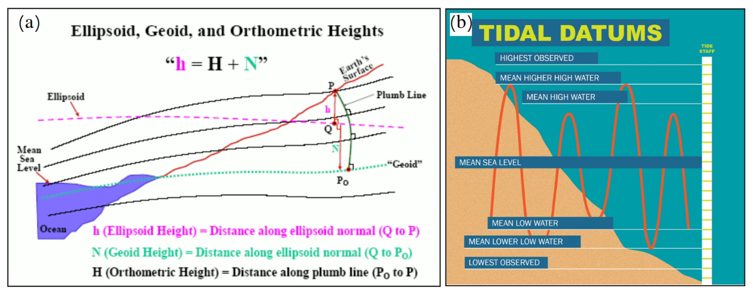
2.1. Surface and Water Elevation Data

Digital elevation models (DEMs) are the representation of land elevation (topographic) or water depth (bathymetric). These datasets serve as the most valuable resources for coastal mapping applications [36]. The process of SLR inundation mapping deals with the interaction of land and water, and, therefore, relies on not only topographic and bathymetric elevation but also datasets representing water levels [37]. As multiple elevation datasets have to be used in the process, the first challenge is maintaining consistency between them, in terms of their spatial reference. While horizontal datum transformations are basic functionality in most GIS software, vertical datum transformations are less commonly used. However, to map coastal inundation, all datasets must reference elevations in the same system. These reference systems, developed to measure heights and depths on Earth’s surface, are called vertical datums [38]. They can be established using ellipsoidal, orthometric or tidal models. Figure 1a illustrates ellipsoidal model heights (h, N) that use a simplified, geometric surface to represent Earth’s shape and size and orthometric model heights (H), which is a physical, gravimetric model that approximates mean sea level. In the United States, DEMs are created by various government agencies and other actors, in varying detail. This includes local, state, and federal organizations. An overview of this complex data ecosystem is provided by Juhász et al. [39]. While the nationally available 1-arc-second-spatial-resolution-(30 m) National Elevation Dataset is not adequate for accurate coastal inundation mapping, high-resolution datasets are increasingly being created and made available publicly [40]. These provide enough detail to facilitate coastal and marine spatial planning on localized scales. A discussion of DEM resolution in the context of SLR mapping is given by Cooper et al. [41].
Tidal datums reference water levels according to certain tidal stages [38]. While geodetic and orthometric datums are more precise and they can be used over a larger area, tidal levels vary by time and by location; therefore, tidal datums always refer to one particular location. Figure 1b shows common tidal datums, while Table 1 lists the difference in elevation values of a specific tidal station in Virginia Key, FL. The Mean Higher High Water (MHHW) is the average height of the highest tide recorded at a station over a period. It is more meaningful, for example, for land development purposes than lower tidal datums [42]; therefore, it is a common reference datum to measure coastal inundation, as areas that are below the MHHW surface are likely to be flooded daily during a normal high tide. For other purposes—such as permitting—other tidal surfaces, such as the Mean High Water (MHW), are used. Table 1 shows that in Virginia Key, FL, the MHHW surface is 7 cm above the NAVD88 (North American Vertical Datum of 1988) orthometric datum, and 64 cm above the mean sea level at that location. In addition, oceans and seas are not flat surfaces and they deviate locally and regionally, due to land movement, varying temperature, and other factors [43,44]. This necessitates the integration of accurate representation of tidal surfaces in the inundation mapping process, as opposed to using a constant elevation value in modeling the inundation extent. A simple, commonly used approach to generating a digital representation of tidal surfaces is using data from tidal stations (see, e.g., [45]); however, a sufficient number of tidal gauges must be available to cover the study area. Another approach in the United States is to use VDatum, a database and software developed by NOAA, designed to vertically transform geospatial data among a variety of tidal, orthometric, and ellipsoidal vertical datums [46]. However, VDatum covers only the continental United States, Puerto Rico, and the U.S. Virgin Islands; therefore, other areas need to use other approaches to general local tidal surfaces [47]. Software with similar functionality to VDatum exists for other areas, such as the Australian-Coastal-Vertical-Datum-Transformation (AusCoastVDT) Software [48] and the Vertical-Datum Conversion Tool from the Canadian Geodetic Survey [49]. As tidal surfaces are usually sampled at distinct locations, a continuous surface resembling the resolution and spatial reference of other input datasets should be interpolated [29].

2.2. Bathtub Approach to Mapping SLR Inundation

Coastal areas become flooded as they submerge below surrounding water levels, due to the rise in sea levels. This is typically simulated using a “bathtub” approach. This simple model assumes that areas that are below a water reference surface are filled with water, like a bathtub. This approach relies on digital representations of the topography (DEMs) and water surface, as described in Section 2.1. The process can be formalized as follows:
I x , y = 1 if D x , y W x , y 0 if D x , y > W x , y ,
where I is a binary variable indicating whether an area is inundated (1) or not inundated (0) at location ( x , y ) , while D and W are the DEM elevation value and projected water level, respectively, at that location. The bathtub can be “filled” with or without hydrological connectivity. In the latter case, only areas that are connected to the main water body (i.e., the ocean or the sea) are considered flooded. This can be achieved by multiplying I in Equation (1) by C x , y , which represents hydrological connectivity, i.e., whether a location is connected (1) or not connected (0) to the main body of water. Areas where I x , y ( I x , y × C x , y ) can be considered low-lying.
Modeling SLR inundation in a GIS environment is a multi-step process that is usually computed using a combination of standard, cell-based raster operations. While most commonly used desktop GIS software does not have a dedicated tool to perform this task, the process is well-documented and has been described before (see, e.g., [51]). A general flowchart is given in Figure 2. The process relies on three inputs: a raster DEM representing elevation values, a baseline raster surface representing the surface on which the SLR is measured, and a numerical SLR value that represents the rise in sea levels above that reference surface. The MHHW is commonly used as a baseline surface (tidal surface), as it is a reliable reference point for understanding the upper limits of daily tidal fluctuations. We refer to the SLR scenario as an x-meter increase in sea levels above the MHHW. The process starts by creating an increased water surface that is x m above the baseline surface (step 1). With reference to Equation (1), W = t + x , where t is the tidal surface. This new surface W represents the water surface in the bathtub modeling process, to which the topography (DEM) is compared. Next, the water surface is subtracted from the DEM (step 2). The resulting surface is negative if the water surface is below the DEM. In step 3, a cell-based classification is performed that classifies this surface into a binary map where cell values of 1 represent areas that fall below the water surface; in other words, “bathtubs” filled with water. Hydrological connectivity is evaluated in steps 4–6, where the binary map produced in step 3 is first recategorized by grouping cells that form physically discrete areas together. Then, categories that represent inundated areas connected to the main body of water are retained. The surface is identical to I in Equation (1). Subsequent steps are optional, but can be used for specific purposes. For example, projected water depths can be generated by using I as a mask surface to overlay with the water depth surface generated in step 2. Additionally, a raster-to-vector conversion can be used to extract inundation polygons, to use in vector-based spatial operations and visualization (step 8).

2.2.1. Limitations of the Bathtub Mapping Approach

While the passive inundation modeling approach provides a valuable tool for understanding potential flood risks in various scenarios, it has its inherent limitations. These are given below:
  • The approach relies on static input data; however, over time, natural and artificial processes can significantly alter the landscape, potentially leading to inaccurate flood predictions.
  • The approach does not consider the dynamic interplay of water flow, wave action, and wind. This can lead to an oversimplification of flood scenarios, especially in areas prone to storm surges or rapidly changing water levels.
  • We assume a universal rise in water levels across the entire study domain; however, factors such as tidal variations, river discharges, and localized rainfall can cause significant disparities in water-level changes across a region. This is more prominent over large study areas.
  • The accuracy and resolution of the data inputs, such as DEMs, directly impact the reliability of passive inundation models.
  • The current approach does not account for spatial variations in land cover and other environmental factors; however, the grid-based approach can be extended to include these.
It is essential for researchers and policymakers to recognize these limitations when interpreting results from passive inundation models. While they offer valuable insights, they should ideally be used in conjunction with other modeling techniques and real-world data for a comprehensive understanding of flood risks.

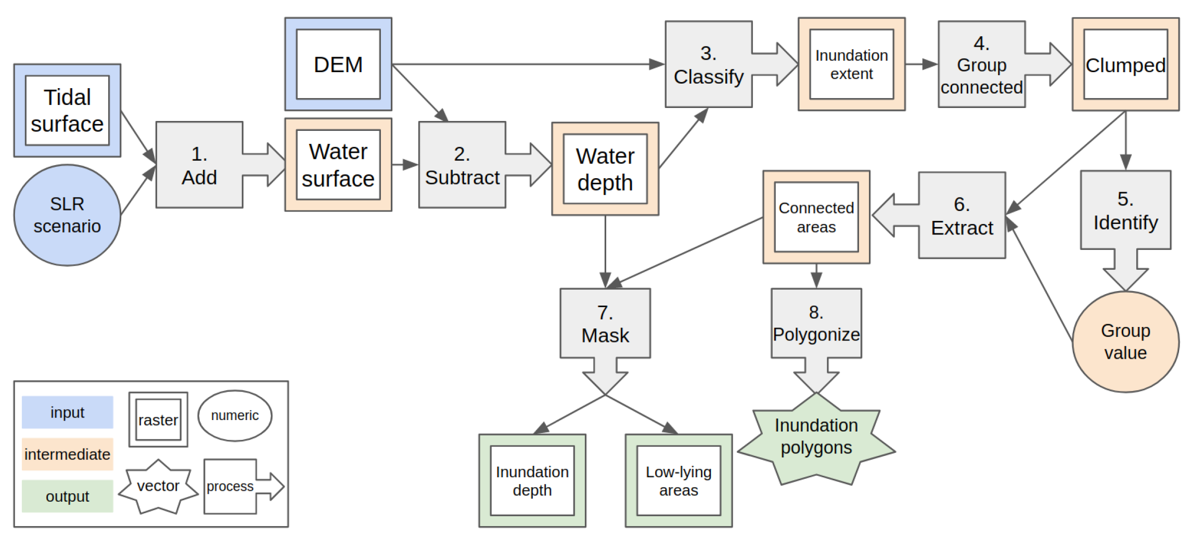
2.3. FOSS4G Implementation

While the implementation of the bathtub approach has been described before, it has been mainly done with proprietary tools, such as the ESRI ArcGIS suite of software [29,47,51]. In this section, we describe an alternative environment that utilizes FOSS4G software tools to implement bathtub modeling of SLR inundation.

Software and Tools

Our implementation uses three widely used FOSS4G software frameworks: namely, GDAL/OGR, GRASS GIS, and QGIS. These software frameworks represent an ensemble of geospatial tools and algorithms, each purpose-built to excel in specific geospatial tasks, such as raster algebra, vectorization, data transformation, and more. It is the seamless integration and collaboration among these tools and algorithms that culminate in the creation of a comprehensive desktop GIS software solution.
In essence, GDAL/OGR (https://gdal.org, accessed on 3 November 2023) provides abstract data models, to represent raster and vector geospatial data. It also contains useful utility tools, to translate between formats as well as to process data [52]. GDAL/OGR facilitates seamless integration into scientific workflows, enabling spatial data professionals to efficiently manage and extract meaningful insights from complex geospatial datasets.
GRASS GIS (https://grass.osgeo.org, accessed on 3 November 2023) is a multi-purpose GIS software used for the production, analysis, and presentation of geospatial data. It is among the most comprehensive GIS software available, with its development work dating back to 1982 [53]. With an extensive array of tools for raster and vector data processing, terrain analysis, hydrological modeling, and more, GRASS GIS provides the means to conduct geospatial analyses, all within a flexible and customizable environment. Its integration of geostatistical, image analysis, and visualization capabilities renders it an indispensable tool for spatial research.
QGIS (https://qgis.org, accessed on 3 November 2023) is desktop GIS software widely employed in scientific research, due to its robust geospatial data handling capabilities and extensive analytical tools [54]. Offering a user-friendly interface, QGIS enables researchers to visualize, analyze, and manipulate spatial data. Its adaptability through plugins and support for numerous data formats further enhances its utility, facilitating complex geospatial analyses and fostering collaborative scientific exploration. In addition to its native algorithms, QGIS also provides an interface to run GDAL/OGR and GRASS GIS algorithms.
All three software frameworks were released as open-source software and are official projects of the Open Source Geospatial Foundation (OSGeo (https://osgeo.org, accessed on 3 November 2023)), which is an umbrella organization that fosters the development and promotion of open-source geospatial technologies and supports collaborative efforts within the geospatial community. These software frameworks can be interfaced in various ways. GDAL/OGR, QGIS, and GRASS GIS all provide application programming interfaces (APIs) that allow the integration of their algorithms into custom-built software. However, this can be considered advanced use-case, and for end uses such as GIS analysts and coastal professionals, this is usually not necessary. More convenient ways to access the functionality necessary for coastal inundation mapping are through graphical user interfaces (GUIs), such as desktop software environments, and through the command line.
Table 2 relates the general workflow described in Figure 2 to specific software and algorithms. Specific implementation of these steps in the context of the case study presented in Section 2.4 and Section 3 is given in Appendix A and is also provided as supporting material (https://doi.org/10.17605/OSF.IO/XEPGR, accessed on 3 November 2023).

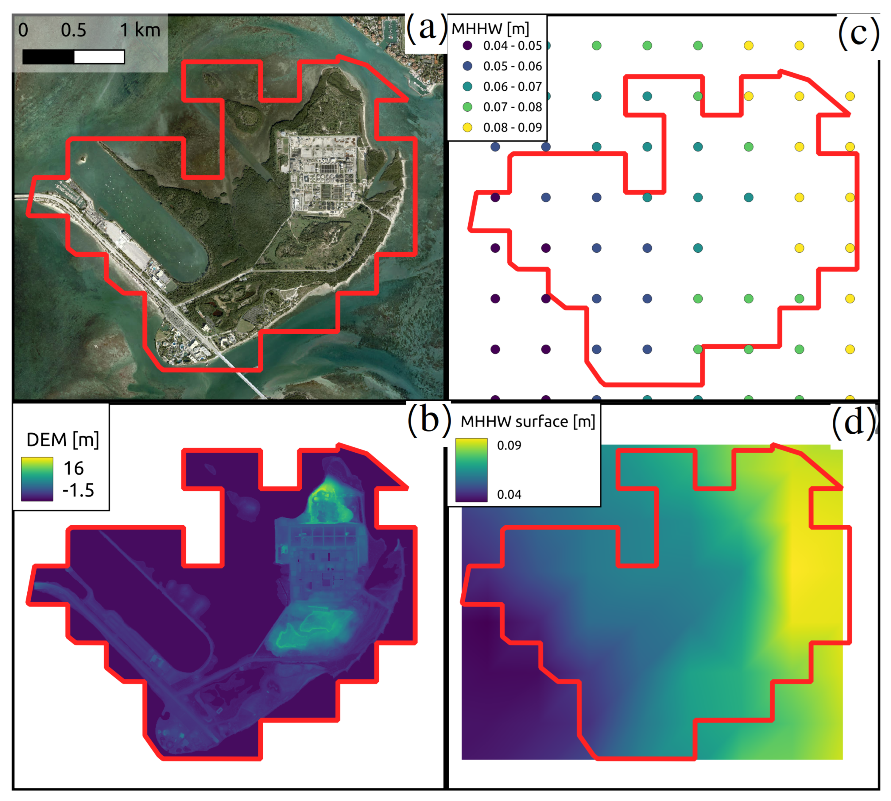
2.4. Description of the Case Study

We demonstrate the implementation with a case study in Virginia Key, which is an approximately 3.5 km2 barrier island in Miami, FL, USA. The island constitutes a mix of built-up and natural areas and houses the Miami Seaquarium and a wastewater facility, as well being home to large mangrove wetlands. NOAA tidal station #8723214 (https://tidesandcurrents.noaa.gov/stationhome.html?id=8723214, accessed on 3 November 2023) is located on the southern part of the island. We adapted the extrapolated intermediate-sea-level scenario specific to this location for the year 2060. The amount of SLR was 0.44 m (1.44 ft). In the USA, this can be determined for each tidal station with sufficient observations, using the Interagency Sea Level Rise Scenario Tool maintained by NASA (https://sealevel.nasa.gov/task-force-scenario-tool?psmsl_id=1858, accessed on 3 November 2023). Other scenarios and detailed methodological description of determining SLR are given by Sweet et al. [55]. It should be noted that for the same year (2060) there are significant differences between scenarios ranging from 0.3 m (low) to 0.69 m (high). The other main input was a LiDAR-based, bare-earth, hydro-enforced DEM provided by Miami-Dade County from 2021 [56]. Elevation values were referenced in meters in relation to NAVD88.
As areas below the MHHW are susceptible to inundation, we used this surface to identify inundated areas. The MHHW was determined at the Virginia Key tidal station and was 0.07 m above the NAVD88 reference surface [50]. However, the ocean is not a flat surface, and there can be a significant amount of variation in the height of tidal surfaces [57]. For this reason, we sampled the MHHW at multiple locations and interpolated a continuous tidal surface, using these distinct points. The MHHW was also expressed in meters, in reference to NAVD88. Section 3 demonstrates this process for Virginia Key. Step-by-step instructions are provided in Appendix A.

3. Results

3.1. Preparation of the Datasets

As described in Section 2.1, coastal inundation modeling requires high-quality input-elevation datasets that represent various surfaces. The DEM representing ground elevations was reprojected to the North American Datum 1983 (NAD83)/Universal Transverse Mercator (UTM) zone 17N coordinate system and resampled to 2.5 m pixel resolution, using gdal_translate (https://gdal.org/programs/gdal_translate.html, accessed on 3 November 2023). This resolution balances computational efficiency and results. Previous studies conducted in Southeast Florida routinely utilized 5 m spatial resolution DEMs [51,58,59]; therefore, our choice can be considered adequate for local-scale modeling of inundation. The study area and the corresponding DEM is shown in Figure 3a,b. The difference in elevation within the study area is  17 m between the lowest and highest points. The highest elevation area is located within the coastal dunes of the northern tip of the island.
While a common approach is using the MHHW surface value from the nearest tidal station as a reference, we recognize that MHHW varies in space. We used NOAA’s VDatum software to sample the MHHW at distinct locations shown in Figure 3c around the study area. VDatum was used to convert between orthometric and tidal datums, more specifically we expressed the MHHW in reference to NAVD88 so that the elevations could be directly compared to the DEM. Figure A3 shows the correct setup to transform MHHW to NAVD88 values in VDatum. It has to be noted that the VDatum coverage area did not extend far beyond the shoreline. Unlike our study area, coastal mapping projects may aim to extend inland, which requires special steps to extend the tidal surface inland as well [29,60]. In the next step, we used the TIN (Triangulated Irregular Network) approach to interpolate a continuous surface, using the same spatial reference and pixel size as the DEM. The TIN is an exact interpolation technique that retains the sampled values at those locations, and returns the interpolated elevation value based on linear interpolation between the sampled points within each triangle of the network. The interpolated surface is shown in Figure 3d. The difference between the MHHW was 5 cm between the Biscayne Bay and Atlantic sides of the study area. While this seems negligible, it already represents 11% of the projected SLR value in 2060. In addition, the difference over larger study areas can be more significant, which highlights the importance of using a more refined MHHW surface than using a constant value across the entire study area.
After preparing these datasets, all inputs of the modeling approach (see Figure 2) were available. The SLR value for the intermediate scenario in 2060 was 0.44 m. The DEM and the MHHW surface were available as single-band rasters in the NAD83 / UTM Zone 17N coordinate system with 2.5 m pixel resolution, pixel values representing MHHW elevations above NAVD88 orthometric datum.

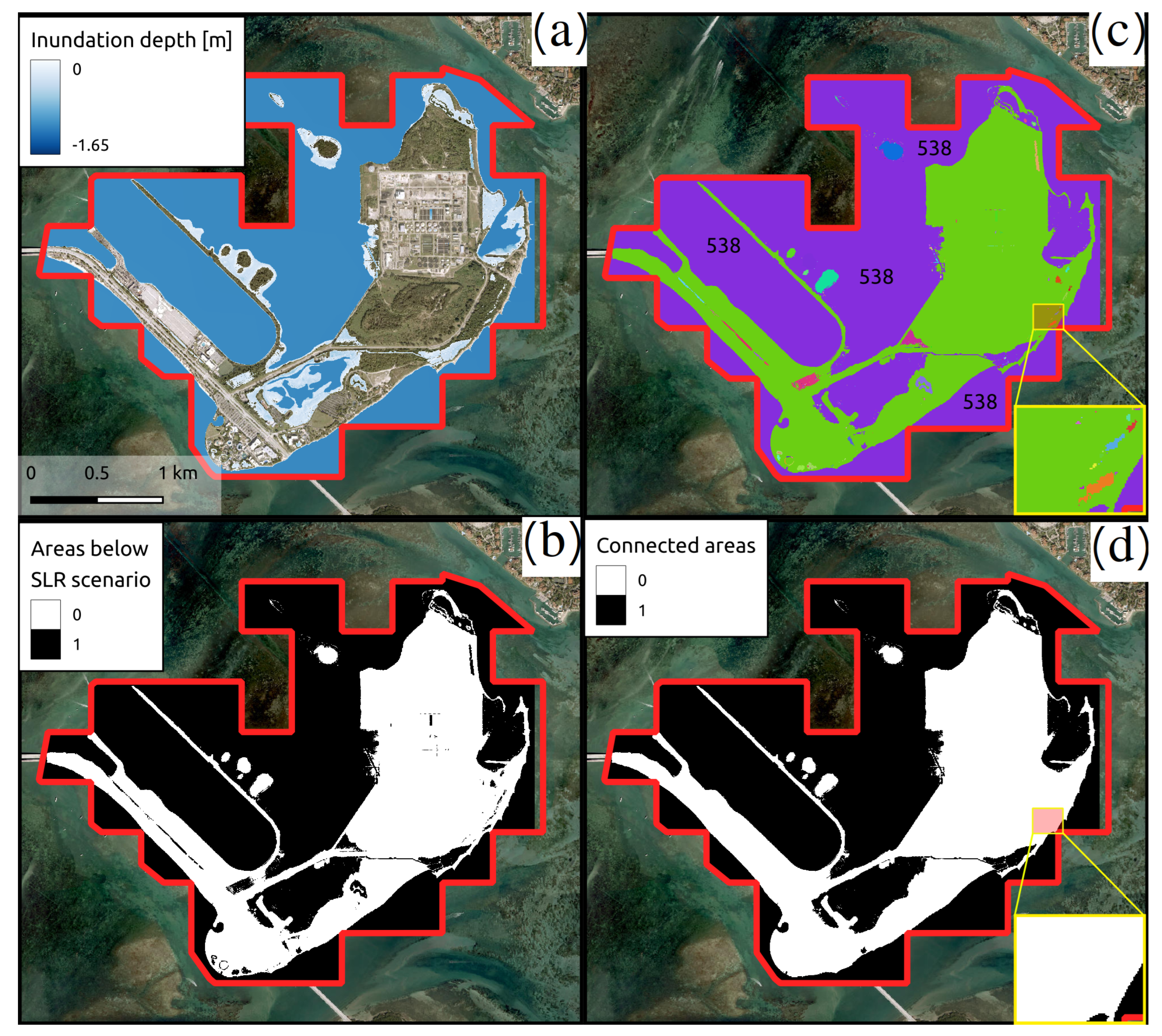
3.2. Simulating SLR Inundation

The SLR scenario value (0.44 m) could be added to the interpolated MHHW surface, using cell-based raster algebra. The new water surface represented MHHW in 2060 according to the intermediate SLR scenario (step 1). Equation (1) was implemented in two steps, first by subtracting the new water surface (W) from the DEM (D) (step 2), then evaluating pixel values to determine inundation extent (step 3). Figure 4a shows the inundation depth after step 2. As areas where D > W could not be considered inundated, these values were retained as 0. In step 3, a binary map was created, where negative values were reclassified and given the value of 1, representing areas that were below the SLR scenario (Figure 4b). The previous steps were executed using raster algebra, which is usually implemented in both FOSS and GIS software. GDAL provided a command-line interface through the gdal_calc python script (https://gdal.org/programs/gdal_calc.html, accessed on 3 November 2023). This was also accessible from the QGIS GUI in addition to QGIS’ own implementation.
Next, the hydrological connectivity was evaluated. The pixels in the the binary water extent map generated in step 3 (Figure 4b) took the value of 1 if the pixel was below the SLR scenario (hence, potentially inundated) or 0 if it lay above the SLR scenario (i.e., not inundated). Neighboring inundated cells could be grouped together to form physically distinct areas with the r.clump GRASS GIS algorithm (step 4). This tool finds all contiguous areas of the same cell value and assigns a unique category to these areas (also referred to as “clumps”). Figure 4c illustrates clumps within the study area. Unique categories are distinguished with different colors. In this figure, the category representing the main body of water is shown in purple, with the category ID 538. Identifying this category is a manual process and can be done in the QGUS GUI through the Identify tool (step 5).
Once the category number of the water body was identified in the clumped map, this area could be used to extract hydrologically connected areas (step 6). This was done by reclassifying the clumped raster map into a binary map, using gdal_calc. The result map is shown in Figure 4d. The difference between this output and the previously created map in Figure 4b is that inland areas below the SLR scenario were removed.
In step 7, the connected-areas raster layer could be used as a mask to extract low-lying areas that were below the SLR scenario but not hydrologically connected, as well as to exclude these areas from the inundation-depth raster created earlier, in step 2 (Figure 4a).
In step 8, raster–vector conversion was performed on the binary inundation map from step 3 and the connected-areas map from step 6. This conversion was done using the r.to.vect function available in GRASS GIS. The conversion process transformed the low-lying areas and the hydrologically connected areas from binary rasters into vector polygons. These vector datasets were more suitable for certain spatial analyses and could be integrated with other vector-based datasets for a comprehensive assessment. Other advantages of the vector format in this context are the potentially smaller size of the dataset over larger areas as well as vector-based visualization techniques. Visualization options are explored in Section 3.3 below.

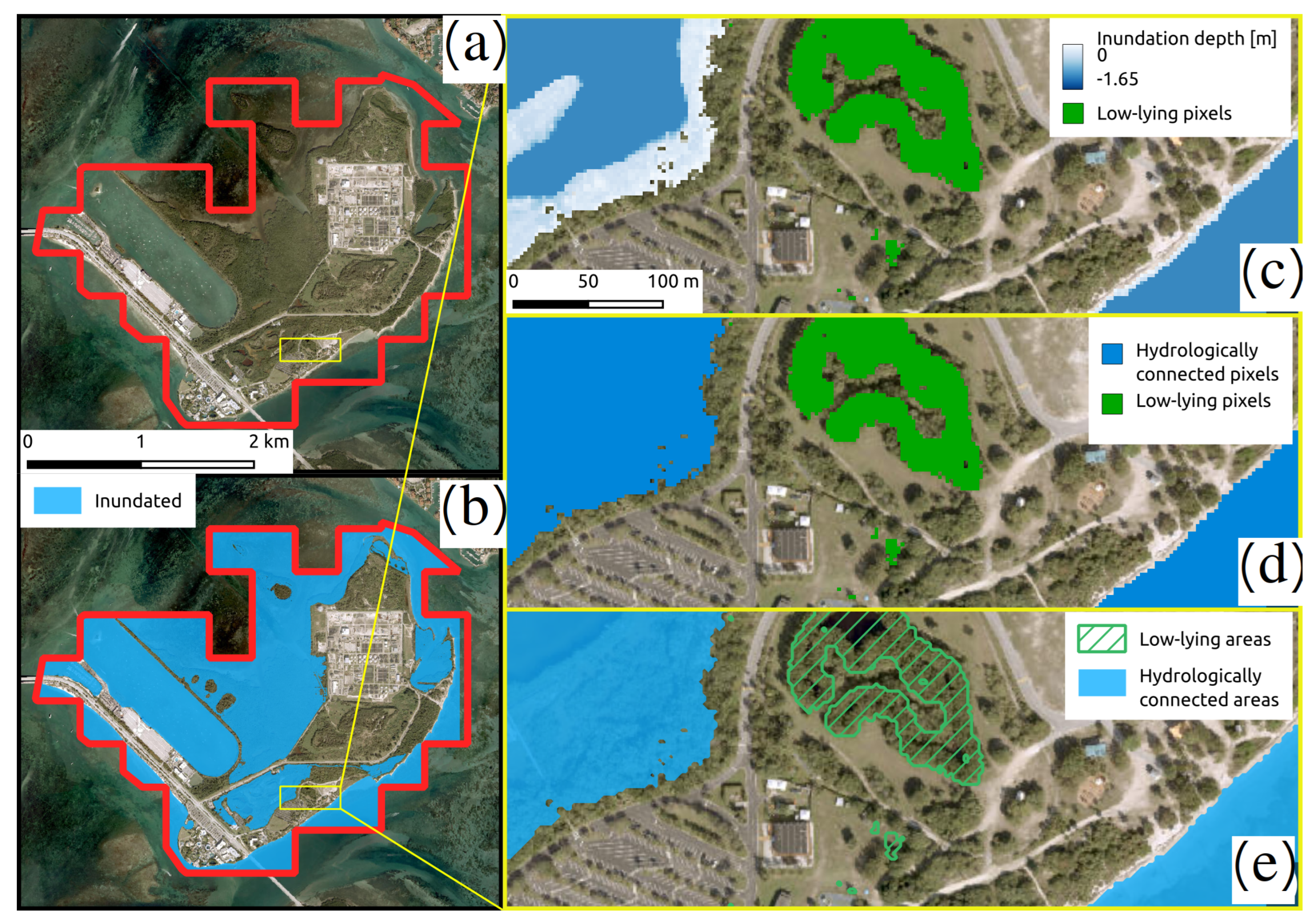
3.3. Visualization of SLR and Low-Lying Areas

Figure 5a,b show the study area with and without displaying coastal inundation under the 2060 intermediate SLR scenario (+0.44 m). SLR inundation is usually visualized using pre-rendered outputs similar to Figure 4a. There are two main approaches. First, similarly to Figure 4a and Figure 5c, inundation depth can be displayed with graduated colors. This approach was popularized by NOAA’s Sea Level Rise Viewer (https://coast.noaa.gov/slr/, accessed on 3 November 2023) [61] that can display the SLR for the contiguous United States. Furthermore, NOAA also allows the integration of these visuals into other applications by serving the data through application programming interfaces (APIs), OGC-(Open Geospatial Consortium)-compliant services, and ESRI-compatible maps. This allows other users to ingest SLR visualizations within their own GIS system [61]. A similar approach, shown in Figure 5d, displays pre-rendered, cell-based raster images, using a single color to represent inundated areas. Low-lying areas can be displayed with both of these approaches.
As described in Section 3.2, inundated and low-lying areas can also be converted into vector polygons, which opens up the flexibility of visualizing vector datasets. An example is given in Figure 5e, where in addition to the semi-transparent inundation polygon, low-lying areas are symbolized with dashed polygons. Outside of desktop GIS environments, the flexibility of vector visualization can be exploited in interactive web applications that show the impact of SLR [39].

4. Discussion and Conclusions

The escalating threat of sea-level rise due to climate change underscores the need for accurate and accessible tools to predict and visualize potential inundation scenarios. Historically, most studies and applications in this domain have relied heavily on proprietary tools, which often come with significant costs and limited accessibility. This creates barriers, especially for stakeholders in developing nations where resources are constrained, and the need for such tools is pressing.
Our study bridges this gap by presenting a comprehensive methodology for mapping SLR inundation using the bathtub approach, but with a distinct emphasis on leveraging the capabilities of free and open-source tools. This democratizes the inundation mapping process, making it accessible to a broader range of users, from researchers in resource-limited settings to local governments in developing nations. The case study of Virginia Key not only demonstrated the practical application of this approach but also emphasized the importance of accounting for spatial variations in tidal surfaces.
While the results derived from the bathtub model provide valuable insights, they are inherently constrained by the static nature of the input data and the absence of dynamic hydrological considerations. However, the adaptability and cost-effectiveness of FOSS4G tools ensure that the generated outputs can be tailored to diverse audiences, from policymakers to local communities.
In conclusion, our work offers a significant contribution by providing an alternative to proprietary tools for SLR inundation mapping. By harnessing the power of FOSS4G tools, we present a solution that is both accessible and customizable, catering especially to those in resource-limited settings. As the global community confronts the challenges of climate change, such tools will be pivotal in driving informed decision making and fostering proactive adaptation strategies.

Author Contributions

Conceptualization, L.J. and R.W.P.; methodology, L.J.; software, L.J.; validation, L.J.; formal analysis, L.J.; investigation, L.J. and J.X.; resources, L.J. and R.W.P.; data curation, L.J.; writing—original draft preparation, L.J. and J.X.; writing—review and editing, L.J., J.X. and R.W.P.; visualization, L.J. All authors have read and agreed to the published version of the manuscript.

Funding

This research was supported by the United States Environmental Protection Agency Region 4 Wetland Development Grant Program (#02D16822).

Institutional Review Board Statement

Not applicable.

Informed Consent Statement

Not applicable.

Data Availability Statement

Sample data and software are available from here: https://doi.org/10.17605/OSF.IO/XEPGR, accessed on 3 November 2023.

Conflicts of Interest

The authors declare no conflict of interest.

Appendix A. FOSS4G Implementation

The dataset as well as two Bash scripts that combine the steps described below are available (https://doi.org/10.17605/OSF.IO/XEPGR, accessed on 10 November 2023). The examples are designed to run on the Ubuntu 22.04 operating system. All software used in the study are platform-independent and can run on any operating system, including Microsoft Windows and macOS. Specific software versions are given below:
  • QGIS 3.34.0-Prizren;
  • GRASS GIS 7.8.7;
  • GDAL/OGR 3.4.1.
Our implementation in the case study utilized the command-line interfaces of this software, except for step 5, which was done manually in the QGIS GUI. However, all steps can be run purely in a desktop environment as well. This is illustrated below for step 1, and can be replicated by the user for the consecutive steps, if desired.

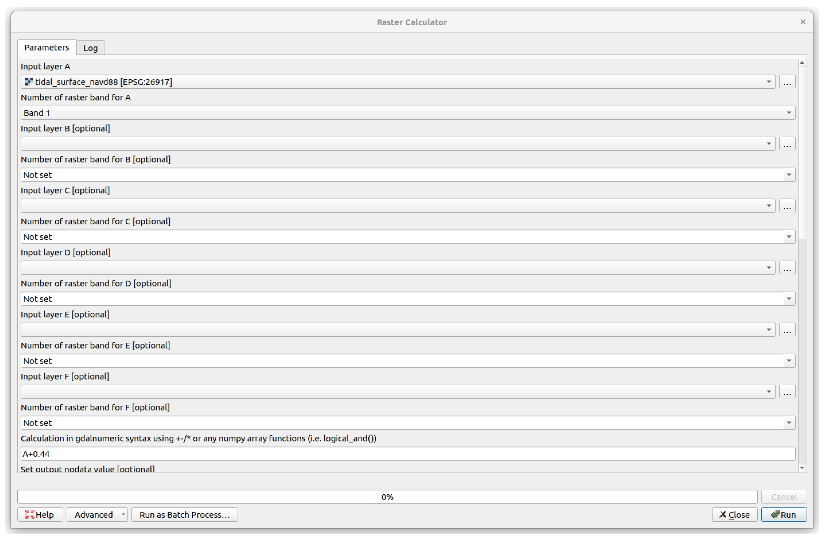
Appendix A.1. Step 1

Listing 1: Using raster algebra with gdal_calc to add a constant value to the tidal surface
  • gdal_calc.py --co COMPRESS=DEFLATE --calc=A+0.44 \
  •     --outfile=water_surface.tif -A tidal_surface_navd88.tif
The command above adds 0.44 (amount of SLR scenario in meters) to the input raster tidal_surface_navd88.tif, using cell-based raster algebra. The -A flag specifies the input dataset, the --calc parameter contains the raster algebra expression, in this case a simple addition operation. The -co COMPRESS=DEFLATE flag applies the DEFLATE lossless compression method to the output GeoTIFF. Figure A1 illustrates how to run the same tool within the QGIS GUI.
Figure A1. Running gdal_calc in QGIS.
Geomatics 03 00028 g0a1

Appendix A.2. Step 2

Listing 2: Using raster algebra with gdal_calc to calculate inundation depth
  • gdal_calc.py --co COMPRESS=DEFLATE --calc="(A <= B) ∗ (A - B)" \
  •     --outfile=depth.tif -A project_dem_metric.tif \
  •     -B water_surface.tif
The command above uses the DEM (project_dem_metric.tif) and the output of step 1 (water_surface.tif) labeled as A and B, respectively. The expression evaluates whether the DEM <= MHHW increases with the SLR scenario, and, if so, subtracts those values resulting in the water depth. All other values are retained as 0s, as the logical multiplier A <= B evaluates to 0.

Appendix A.3. Step 3

Listing 3: Using raster algebra with gdal_calc to create a binary inundation raster
  • gdal_calc.py --co COMPRESS=DEFLATE --calc="(A <= B) ∗ 1" \
  •     --outfile=single.tif -A project_dem_metric.tif \
  •     -B water_surface.tif
Instead of retaining water depth, this command generates a binary water extent raster.

Appendix A.4. Step 4

  • Listing 4: Running the r.clump GRASS GIS algorithm through a QGIS process on the command line
  • qgis_process run grass7:r.clump --distance_units=meters \
  •     --area_units=m2 --ellipsoid=EPSG:7019 --input=single.tif \
  •     --title=clumped.tif ---d=true --output=clumped.tif \
  •     --threshold=0 --GRASS_REGION_CELLSIZE_PARAMETER=0 \
  •     --GRASS_RASTER_FORMAT_OPT=‘COMPRESS=DEFLATE’
Grouping connected cells is done by running the r.clump GRASS GIS algorithm. Although GRASS GIS can be run natively, the command above uses the QGIS Process Executor engine. The advantage of this approach is that data conversion from GeoTIFF to GRASS’ native format and other settings are handled automatically.

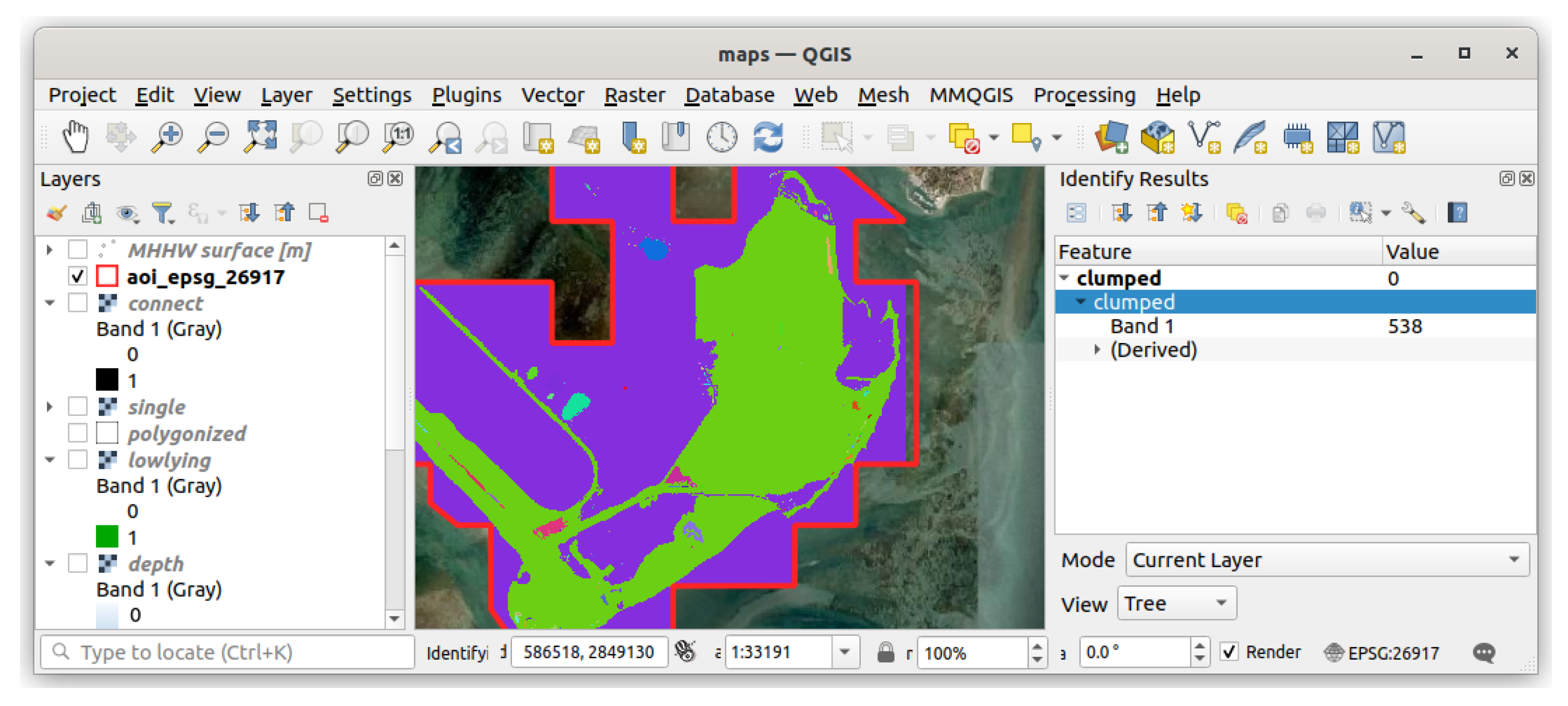
Appendix A.5. Step 5

The water surface can be visually identified in QGIS, using the Identify tool (Figure A2). In the case study, this corresponds to the value of 538.
Figure A2. Identifying the category representing the water extent in QGIS.
Geomatics 03 00028 g0a2

Appendix A.6. Step 6

  • Listing 5: Using raster algebra with gdal_calc to retain hydrologically connected areas
  • gdal_calc.py --NoDataValue "65535" --co COMPRESS=DEFLATE \
  •     --calc="(A == 538) ∗ 1" --outfile=connect.tif -A clumped.tif
The command above uses the category identified in the previous step. It retains pixels with the value of 1 if they belong to the hydrologically connected main body of water. All other pixels are classified as 0.

Appendix A.7. Step 7

Listing 6: Using raster algebra with gdal_calc to retain low-lying areas
  • gdal_calc.py --NoDataValue "65535" --co COMPRESS=DEFLATE \
  •     --calc="(A == 1) ∗ (B == 0) " --outfile=lowlying.tif \
  •     -A single.tif -B connect.tif
The command above retains low-lying areas with the pixel value of 1 by comparing the hydrologically connected output from the previous step with areas that are below the SLR scenario (step 3).

Appendix A.8. Step 8

  • Listing 7: Running the r.to.vect GRASS GIS algorithm through a QGIS process to vectorize a rester
  • qgis_process run grass7:r.to.vect --distance_units=meters \
  •     --area_units=m2 --ellipsoid=EPSG:7019 --input=connect.tif \
  •     --type=2 --column=value ---s=true ---v=false ---z=false \
  •     ---b=false ---t=false --output=polygonized.shp \
  •     --GRASS_REGION_CELLSIZE_PARAMETER=0 \
  •     --GRASS_OUTPUT_TYPE_PARAMETER=3 --GRASS_VECTOR_DSCO= \
  •     --GRASS_VECTOR_LCO= --GRASS_VECTOR_EXPORT_NOCAT=false
Listing 8: Using ogr2ogr to filter inundated areas from vectorized polygons
  • ogr2ogr -where "\"cat\" = 1" inundated.shp polygonized.shp
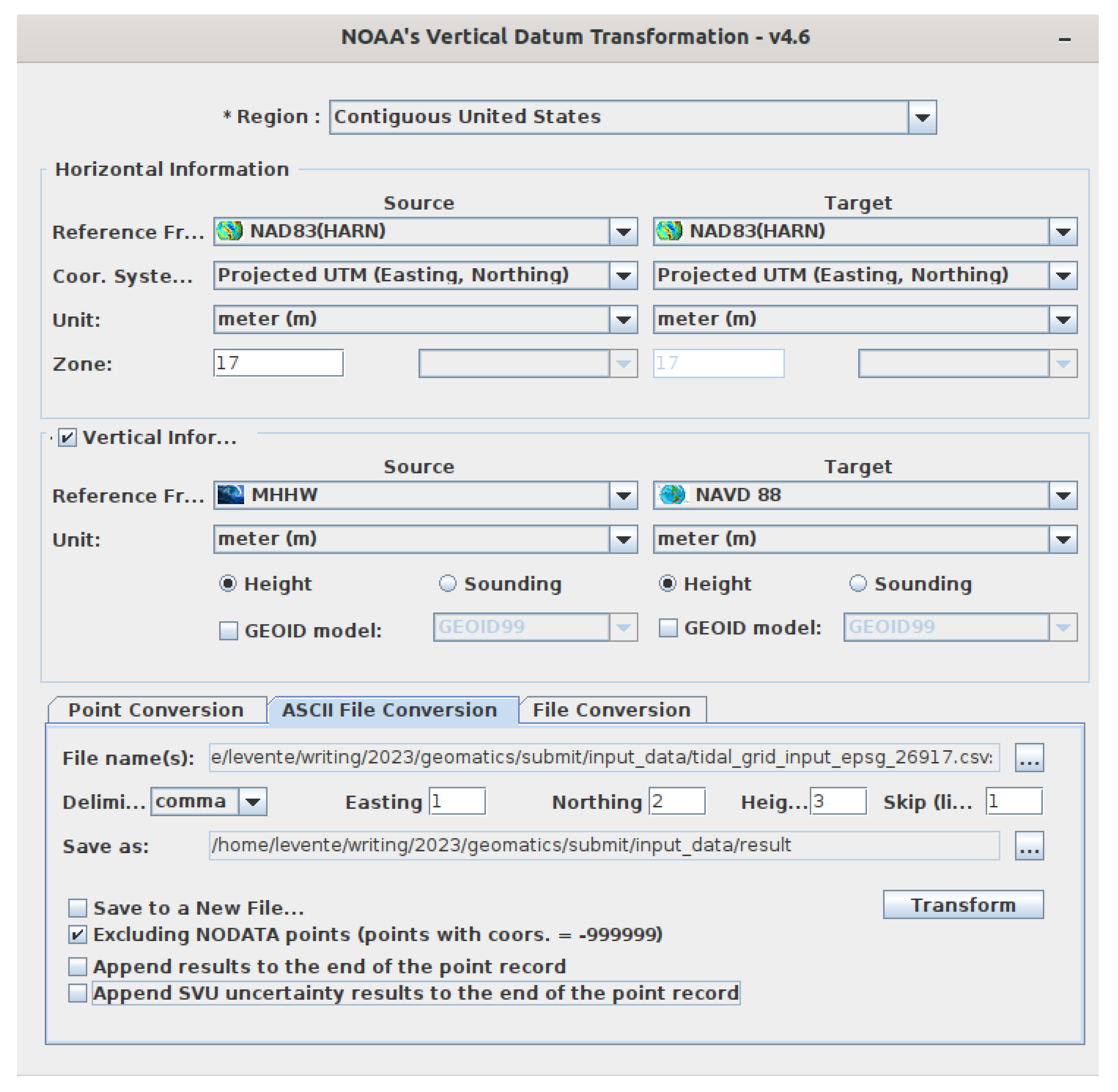
In a two-step process, first the GRASS GIS algorithm r.to.vect is used to convert the hydrologically connected raster dataset into an ESRI shapefile. Then, ogr2ogr can be used to retain only the polygons that were created with inundated pixels.

Appendix B. VDatum

Figure A3. Converting local MHHW grid to NAVD88 elevations, using VDatum.
Geomatics 03 00028 g0a3

References

  1. Sobel, A.H.; Camargo, S.J.; Hall, T.M.; Lee, C.Y.; Tippett, M.K.; Wing, A.A. Human influence on tropical cyclone intensity. Science 2016, 353, 242–246. [Google Scholar] [CrossRef] [PubMed]
  2. Xi, D.; Lin, N.; Gori, A. Increasing sequential tropical cyclone hazards along the US East and Gulf coasts. Nat. Clim. Chang. 2023, 13, 258–265. [Google Scholar] [CrossRef]
  3. Overland, J.; Dunlea, E.; Box, J.E.; Corell, R.; Forsius, M.; Kattsov, V.; Olsen, M.S.; Pawlak, J.; Reiersen, L.O.; Wang, M. The urgency of Arctic change. Polar Sci. 2019, 21, 6–13. [Google Scholar] [CrossRef]
  4. Bushard, B. Record-Breaking Summer: Jacksonville, Miami Break Daily High Temperature Records, after Hottest July Ever. Forbes. 4 September 2023. Available online: https://www.forbes.com/sites/brianbushard/2023/08/09/miami-phoenix-new-orleans-break-daily-high-temperature-records-heres-where-else-daily-records-have-fallen/ (accessed on 3 November 2023).
  5. Fortin, J.F.; Gahan, M.B. Phoenix Breaks Heat Record Set in 1974. The New York Times. 18 July 2023. Available online: https://www.nytimes.com/2023/07/18/us/phoenix-heat-record.html/ (accessed on 3 November 2023).
  6. Small, C.; Gornitz, V.; Cohen, J.E. Coastal hazards and the global distribution of human population. Environ. Geosci. 2000, 7, 3–12. [Google Scholar] [CrossRef]
  7. Ketabchi, H.; Mahmoodzadeh, D.; Ataie-Ashtiani, B.; Simmons, C.T. Sea-level rise impacts on seawater intrusion in coastal aquifers: Review and integration. J. Hydrol. 2016, 535, 235–255. [Google Scholar] [CrossRef]
  8. Snoussi, M.; Ouchani, T.; Niazi, S. Vulnerability assessment of the impact of sea-level rise and flooding on the Moroccan coast: The case of the Mediterranean eastern zone. Estuar. Coast. Shelf Sci. 2008, 77, 206–213. [Google Scholar] [CrossRef]
  9. Daniels, R.C.; White, T.W.; Chapman, K.K. Sea-level rise: Destruction of threatened and endangered species habitat in South Carolina. Environ. Manag. 1993, 17, 373–385. [Google Scholar] [CrossRef]
  10. Parkinson, R.W.; Wdowinski, S. Accelerating sea-level rise and the fate of mangrove plant communities in South Florida, U.S.A. Geomorphology 2022, 412, 108329. [Google Scholar] [CrossRef]
  11. French, G.T.; Awosika, L.F.; Ibe, C. Sea-level rise and Nigeria: Potential impacts and consequences. J. Coast. Res. 1995, 224–242. [Google Scholar]
  12. Williams, L.L.; Lück-Vogel, M. Comparative assessment of the GIS based bathtub model and an enhanced bathtub model for coastal inundation. J. Coast. Conserv. 2020, 24, 23. [Google Scholar] [CrossRef]
  13. Jelesnianski, C.P. SLOSH: Sea, Lake, and Overland Surges from Hurricanes; NOAA Technical Report NWS 48; US Department of Commerce, National Oceanic and Atmospheric Administration: Silver Spring, MD, USA, 1992. [Google Scholar]
  14. Roelvink, J.; Van Banning, G. Design and development of DELFT3D and application to coastal morphodynamics. Oceanogr. Lit. Rev. 1995, 11, 925. [Google Scholar]
  15. Luettich, R.A.; Westerink, J.J.; Scheffner, N.W. ADCIRC: An Advanced Three-Dimensional Circulation Model for Shelves, Coasts, and Estuaries. Report 1, Theory and Methodology of ADCIRC-2DD1 and ADCIRC-3DL; US Army Corps of Engineers: Washington, DC, USA, 1992. [Google Scholar]
  16. Mcleod, E.; Poulter, B.; Hinkel, J.; Reyes, E.; Salm, R. Sea-level rise impact models and environmental conservation: A review of models and their applications. Ocean. Coast. Manag. 2010, 53, 507–517. [Google Scholar] [CrossRef]
  17. Reyes, E.; White, M.L.; Martin, J.F.; Kemp, G.P.; Day, J.W.; Aravamuthan, V. Landscape modeling of coastal habitat change in the Mississippi Delta. Ecology 2000, 81, 2331–2349. [Google Scholar] [CrossRef]
  18. Martin, J.F.; White, M.L.; Reyes, E.; Kemp, G.P.; Mashriqui, H.; Day, J.W., Jr. Evaluation of Coastal Management Plans with a Spatial Model: Mississippi Delta, Louisiana, USA. Environ. Manag. 2000, 26, 117–129. [Google Scholar] [CrossRef]
  19. Feenstra, J.F. Handbook on Methods for Climate Change Impact Assessment and Adaptation Strategies; United Nations Environment Programme: Nairobi, Kenya, 1998. [Google Scholar]
  20. Cartwright, A.; Brundrit, G.; Fairhurst, L. Global climate change and adaptation—A sea-level rise risk assessment. In Phase Four: Adaptation and Risk Mitigation Measures for the City of Cape Town; Prepared for the City of Cape Town by LaquaR Consultants CC; Stockholm Environment Institute: Stockholm, Sweden, 2008. [Google Scholar]
  21. Hinkel, J.; Nicholls, R.J.; Vafeidis, A.T.; Tol, R.S.; Avagianou, T. Assessing risk of and adaptation to sea-level rise in the European Union: An application of DIVA. Mitig. Adapt. Strateg. Glob. Chang. 2010, 15, 703–719. [Google Scholar] [CrossRef]
  22. Brown, S.; Nicholls, R.J.; Lowe, J.A.; Hinkel, J. Spatial variations of sea-level rise and impacts: An application of DIVA. Clim. Chang. 2016, 134, 403–416. [Google Scholar] [CrossRef]
  23. Juhász, L.; Podolcsák, A.; Doleschall, J. Open Source Web GIS Solutions in Disaster Management–with Special Emphasis on Inland Excess Water Modeling. J. Environ. Geogr. 2016, 9, 15–21. [Google Scholar] [CrossRef]
  24. Ramanayake, K.; Vithanage, D.; Hettiarachchi, N.; Rathnayake, G.; Rajapaksha, S.; Fernando, N. Geo-enabled FOSS tool supports for immediate flood disaster response planning. In Proceedings of the 7th International Conference on Information and Automation for Sustainability, Colombo, Sri Lanka, 22–24 December 2014; pp. 1–6. [Google Scholar] [CrossRef]
  25. Dutta, U.; Singh, Y.K.; Prabhu, T.S.M.; Yendargaye, G.; Kale, R.G.; Kumar, B.; Khare, M.; Yadav, R.; Khattar, R.; Samal, S.K. Flood Forecasting in Large River Basins Using FOSS Tool and HPC. Water 2021, 13, 3484. [Google Scholar] [CrossRef]
  26. Lichter, M.; Felsenstein, D. Assessing the costs of sea-level rise and extreme flooding at the local level: A GIS-based approach. Ocean. Coast. Manag. 2012, 59, 47–62. [Google Scholar] [CrossRef]
  27. Li, X.; Grady, C.; Peterson, A.T. Delineating sea level rise inundation using a graph traversal algorithm. Mar. Geod. 2014, 37, 267–281. [Google Scholar] [CrossRef]
  28. Perini, L.; Calabrese, L.; Salerno, G.; Ciavola, P.; Armaroli, C. Evaluation of coastal vulnerability to flooding: Comparison of two different methodologies adopted by the Emilia-Romagna region (Italy). Nat. Hazards Earth Syst. Sci. 2016, 16, 181–194. [Google Scholar] [CrossRef]
  29. NOAA. Detailed Method for Mapping Sea Level Rise Inundation. In Method Description; NOAA Office for Coastal Management: Washington, DC, USA, 2017. Available online: https://coast.noaa.gov/data/digitalcoast/pdf/slr-inundation-methods.pdf (accessed on 3 November 2023).
  30. Styrin, E.; Luna-Reyes, L.F.; Harrison, T.M. Open data ecosystems: An international comparison. Transform. Gov. People Process. Policy 2017, 11, 132–156. [Google Scholar] [CrossRef]
  31. Rajabifard, A.; Binns, A.; Masser, I.; Williamson, I. The role of sub-national government and the private sector in future spatial data infrastructures. Int. J. Geogr. Inf. Sci. 2006, 20, 727–741. [Google Scholar] [CrossRef]
  32. Goodchild, M.F.; Fu, P.; Rich, P. Sharing geographic information: An assessment of the Geospatial One-Stop. Ann. Assoc. Am. Geogr. 2007, 97, 250–266. [Google Scholar] [CrossRef]
  33. The Geospatial Data Act of 2018. (P.L. 115-254), H.R. 302, Subtitle F, Sections 751–759. 2018. Available online: https://www.fgdc.gov/gda/online#:~:text=Extract%20of%20%E2%80%9CGeospatial%20Data%20Act,F%2C%20Sections%20751%20%E2%80%93%20759 (accessed on 3 November 2023).
  34. Choi, J.; Ahn, J.; Kim, H. A Cross National Comparison on the Awareness of Adopting FOSS4G to NSDI in Developing Countries. In Proceedings of the Free and Open Source Software for Geospatial (FOSS4G) Conference Proceedings, Seoul, Republic of Korea, 14–19 September 2015; Volume 15, p. 36. [Google Scholar] [CrossRef]
  35. NOAA. A Tutorial on Datums. 2023. Available online: https://vdatum.noaa.gov/docs/datums.html (accessed on 3 November 2023).
  36. National Research Council. Mapping the Zone: Improving Flood Map Accuracy; National Academies Press: Washington, DC, USA, 2009. [Google Scholar] [CrossRef]
  37. Gesch, D.B.; Gutierrez, B.T.; Gill, S.K. Coastal Elevations. In Coastal Sensitivity to Sea-Level Rise: A Focus on the Mid-Atlantic Region; Titus, J.G., Anderson, K.E., Cahoon, D.R., Gesch, D.B., Gill, S.K., Gutierrez, B.T., Thieler, E.R., Williams, S.J., Eds.; U.S. Climate Change Science Program: Washington, DC, USA, 2009; pp. 25–42. [Google Scholar]
  38. NOAA. National Tidal Datum Epoch. 2023. Available online: https://tidesandcurrents.noaa.gov/datum-updates/ntde/ (accessed on 3 November 2023).
  39. Juhász, L.; Hochmair, H.H.; de Santana, S.A.; Fu, Z.J. Sea Level Rise Impact Assessment Tool—A Web-Based Application for Community Resilience in Coral Gables, Florida. Int. J. Spat. Data Infrastructures Res. 2020, 15, 36–55. [Google Scholar] [CrossRef]
  40. Danielson, J.J.; Poppenga, S.K.; Tyler, D.J.; Palaseanu-Lovejoy, M.; Gesch, D.B. Coastal National Elevation Database; USGS Fact Sheet 2018–3037; U.S. Geological Survey: Reston, VA, USA, 2018. [Google Scholar] [CrossRef]
  41. Cooper, H.M.; Fletcher, C.H.; Chen, Q.; Barbee, M.M. Sea-level rise vulnerability mapping for adaptation decisions using LiDAR DEMs. Prog. Phys. Geogr. Earth Environ. 2013, 37, 745–766. [Google Scholar] [CrossRef]
  42. Harris, D.L. Tides and Tidal Datums in the United States; Technical Report SR-7; United States Army Corps of Engineers, Coastal Engineering Research Center: Fort Belvoir, VA, USA, 1981. [Google Scholar]
  43. Adhikari, S.; Ivins, E.R.; Frederikse, T.; Landerer, F.W.; Caron, L. Sea-level fingerprints emergent from GRACE mission data. Earth Syst. Sci. Data 2019, 11, 629–646. [Google Scholar] [CrossRef]
  44. Katsman, C.A.; Sterl, A.; Beersma, J.J.; van den Brink, H.W.; Church, J.A.; Hazeleger, W.; Kopp, R.E.; Kroon, D.; Kwadijk, J.; Lammersen, R.; et al. Exploring high-end scenarios for local sea level rise to develop flood protection strategies for a low-lying delta—the Netherlands as an example. Clim. Chang. 2011, 109, 617–645. [Google Scholar] [CrossRef]
  45. Shen, S.; Kim, K. Assessment of Transportation System Vulnerabilities to Tidal Flooding in Honolulu, Hawaii. Transp. Res. Rec. 2020, 2674, 207–219. [Google Scholar] [CrossRef]
  46. Parker, B.; Milbert, D.; Hess, K.; Gill, S. National VDatum—The implementation of a national vertical datum transformation database. In Proceedings of the Proceeding from the US Hydro’2003 Conference, Biloxi, MS, USA, 24–27 March 2003; Available online: https://vdatum.noaa.gov/download/publications/2003_parker_USHydro_nationalvdatum.pdf (accessed on 3 November 2023).
  47. Paoa, N.; Fletcher, C.H.; Anderson, T.R.; Coffman, M.; Habel, S. Probabilistic sea level rise flood projections using a localized ocean reference surface. Sci. Rep. 2023, 13, 2257. [Google Scholar] [CrossRef]
  48. SeaGIS. AusCoastVDT, Software Version 1.20, Grid Version 3.0, User Manual Version 1.3. 2019. Available online: https://www.icsm.gov.au/sites/default/files/AusCoastVDT_v1.20.zip (accessed on 3 November 2023).
  49. Canadian Geodetic Survey. Vertical Datum Transformations. 2022. Available online: https://webapp.csrs-scrs.nrcan-rncan.gc.ca/geod/data-donnees/datum-transformation.php?locale=en (accessed on 3 November 2023).
  50. NOAA. NOAA/NOS/CO-OPS Datums for Station 8723214, Virginia Key, Biscayne Bay FL. 2023. Available online: https://tidesandcurrents.noaa.gov/datums.html?id=8723214 (accessed on 3 November 2023).
  51. Zhang, K.; Dittmar, J.; Ross, M.; Bergh, C. Assessment of sea level rise impacts on human population and real property in the Florida Keys. Clim. Chang. 2011, 107, 129–146. [Google Scholar] [CrossRef]
  52. Warmerdam, F. The geospatial data abstraction library. In Open Source Approaches in Spatial Data Handling; Advances in Geographic Information Science; Hall, G.B., Leahy, M.G., Eds.; Springer: Berlin/Heidelberg, Germany, 2008; Volume 2, pp. 87–104. [Google Scholar] [CrossRef]
  53. Neteler, M.; Bowman, M.H.; Landa, M.; Metz, M. GRASS GIS: A multi-purpose open source GIS. Environ. Model. Softw. 2012, 31, 124–130. [Google Scholar] [CrossRef]
  54. Flenniken, J.M.; Stuglik, S.; Iannone, B.V. Quantum GIS (QGIS): An introduction to a free alternative to more costly GIS platforms: FOR359/FR428, 2/2020. EDIS 2020, 2020, 7. [Google Scholar] [CrossRef]
  55. Sweet, W.; Hamlington, B.; Kopp, R.; Weaver, C.; Barnard, P.; Bekaert, D.; Brooks, W.; Craghan, M.; Dusek, G.; Frederikse, T.; et al. Global and Regional Sea Level Rise Scenarios for the United States: Updated Mean Projections and Extreme Water Level Probabilities Along U.S. Coastlines; NOAA Technical Report NOS 01; National Oceanic and Atmospheric Administration, National Ocean Service: Silver Spring, MD, USA, 2022. [Google Scholar]
  56. GPI Geospatial Inc. Miami-Dade County LiDAR DEM; Miami-Dade Open Data Hub: Miami, FL, USA, 2021; Available online: https://mdc.maps.arcgis.com/home/item.html?id=8c48d4bb8d9a42908f4936f698a2961a (accessed on 3 November 2023).
  57. Gill, S.K.; Schultz, J.R. Tidal Datums and Their Applications; Report; NOAA, NOS Center for Operational Oceanographic Products and Services: Washington, DC, USA, 2001. [Google Scholar] [CrossRef]
  58. Zhang, K. Analysis of non-linear inundation from sea-level rise using LIDAR data: A case study for South Florida. Clim. Chang. 2011, 106, 537–565. [Google Scholar] [CrossRef]
  59. Ann Conyers, Z.; Grant, R.; Roy, S.S. Sea level rise in Miami Beach: Vulnerability and real estate exposure. Prof. Geogr. 2019, 71, 278–291. [Google Scholar] [CrossRef]
  60. NOAA. Technical Considerations for Use of Geospatial Data in Sea Level Change Mapping and Assessment; NOAA Technical Report NOS 2010-1; NOAA: Washington, DC, USA, 2010. [Google Scholar]
  61. Marcy, D.; Brooks, W.; Draganov, K.; Hadley, B.; Haynes, C.; Herold, N.; McCombs, J.; Pendleton, M.; Ryan, S.; Schmid, K.; et al. New Mapping Tool and Techniques for Visualizing Sea Level Rise and Coastal Flooding Impacts. In Solutions to Coastal Disasters 2011; ASCE: Anchorage, AK, USA, 2011; pp. 474–490. [Google Scholar] [CrossRef]
Figure 1. Illustration of referencing elevation data to different vertical datums (a) [35] and commonly used tidal datums (b) [38].
Geomatics 03 00028 g001
Figure 2. General workflow of the SLR mapping process.
Geomatics 03 00028 g002
Figure 3. Satellite photo of the Virginia Key study area (red outline) (a). LiDAR-based DEM of the study area with NAVD88 elevations (b). Locations where MHHW was sampled (NAVD88) (c). Interpolated, continuous MHHW surface (d).
Geomatics 03 00028 g003
Figure 4. Inundation depth is calculated by subtracting an SLR scenario from the DEM of the study area (a). Binary map showing pixels below SLR-increased MHHW (b). Grouping cells that form physically discrete areas into ‘clumps’ (c). Binary inundation map representing areas that are hydrologically connected to the main body of water (d).
Geomatics 03 00028 g004
Figure 5. Satellite view of Virginia Key, FL (a). Inundated areas in Virginia Key under the 2060 intermediate scenario (+0.44 m) (b). SLR visualization methods using graduated colors (raster) (c), simple colors (raster) (d), and vector polygons (e).
Geomatics 03 00028 g005
Table 1. Tidal datums for Virginia Key, Biscayne Bay, FL Tidal Station (#8723214) for Tidal Epoch 1983–2001 along with their relative elevation values compared to Mean Higher High Water [50].
DatumDescriptionValue [m]
Max. TideHighest Observed Tide1.09
MHHWMean Higher High Water0.00
MHWMean High Water−0.02
NAVD88 1North American Vertical Datum of 1988−0.07
MSLMean Sea Level−0.34
MLWMean Low Water−0.64
MLLWMean Lower Low Water−0.68
Min. TideMinimum Observed Tide−1.08
STDTStation Datum−3.77
1 NAVD88 is an orthometric datum.
Table 2. Steps of SLR inundation mapping workflow with FOSS4G tools.
Step DescriptionInput(s)Output(s)SoftwareTool
1Add SLR scenario to tidal
surface raster
Tidal surface (raster)
SLR value (numeric)
Water surface (raster)GDALgdal_calc
2Subtract DEM from water
surface
Water surface (raster)
DEM
Inundation depth (raster)GDALgdal_calc
3Create inundation extentInundation depth (raster)
DEM
Binary water extent (raster)GDALgdal_calc
4Group connected cellsBinary water extent (raster)Clumped (raster)GRASS GISr.clump
5Identify hydrologically
connected areas
Clumped (raster)Max value (numeric)QGIS
GDAL
identify
gdalinfo
6Extract hydrologically
connected water surface
Clumped (raster)
Max value (numeric)
Connected areas (raster)GDALgdal_calc
7Conflate water depth with
inundation mask
Connected areas (raster)
Water depth (raster)
Inundation depth (raster)
Low-lying areas (raster)
GDALgdal_calc
8 *Polygonize inundation extentInundated areas (raster)Inundation areas (vector)GRASS GIS
GDAL/OGR
r.to.vect
ogr2ogr
* Optional steps.
Disclaimer/Publisher’s Note: The statements, opinions and data contained in all publications are solely those of the individual author(s) and contributor(s) and not of MDPI and/or the editor(s). MDPI and/or the editor(s) disclaim responsibility for any injury to people or property resulting from any ideas, methods, instructions or products referred to in the content.

