Article

Comparative Analysis of Algorithms to Cleanse Soil Micro-Relief Point Clouds

by
Simone Ott
1,*,
Benjamin Burkhard
1,
Corinna Harmening
2,
Jens-André Paffenholz
3 and
Bastian Steinhoff-Knopp
4
1
Institute of Physical Geography and Landscape Ecology, Leibniz University of Hannover, 30167 Hannover, Germany
2
Geodetic Institute Karlsruhe (GIK), Karlsruhe Institute of Technology (KIT), 76131 Karlsruhe, Germany
3
Institute of Geo-Engineering, Clausthal University of Technology (TUC), 38678 Clausthal-Zellerfeld, Germany
4
Coordination Unit Climate and Soil, Thünen-Institute, 38116 Braunschweig, Germany
*
Author to whom correspondence should be addressed.
Geomatics 2023, 3(4), 501-521; https://doi.org/10.3390/geomatics3040027
Submission received: 11 October 2023 / Revised: 20 November 2023 / Accepted: 23 November 2023 / Published: 26 November 2023

Abstract

:
Detecting changes in soil micro-relief in farmland helps to understand degradation processes like sheet erosion. Using the high-resolution technique of terrestrial laser scanning (TLS), we generated point clouds of three 2 × 3 m plots on a weekly basis from May to mid-June in 2022 on cultivated farmland in Germany. Three well-known applications for eliminating vegetation points in the generated point cloud were tested: Cloth Simulation Filter (CSF) as a filtering method, three variants of CANUPO as a machine learning method, and ArcGIS PointCNN as a deep learning method, a sub-category of machine learning using deep neural networks. We assessed the methods with hard criteria such as F1 score, balanced accuracy, height differences, and their standard deviations to the reference surface, resulting in data gaps and robustness, and with soft criteria such as time-saving capacity, accessibility, and user knowledge. All algorithms showed a low performance at the initial measurement epoch, increasing with later epochs. While most of the results demonstrate a better performance of ArcGIS PointCNN, this algorithm revealed an exceptionally low performance in plot 1, which is describable by the generalization gap. Although CANUPO variants created the highest amount of data gaps, we recommend that CANUPO include colour values in combination with CSF.

1. Introduction

The importance of healthy soils is impossible to overestimate, as it is the foundation of food security and many other life-sustaining ecosystem services. One major driving factor of soil degradation is the process of soil erosion. Current global rates of soil erosion are already far above the natural soil formation rates. Moreover, climate change, as well as land use changes, will exacerbate the situation [1,2].
Knowledge about drivers and actual soil erosion rates at the local scale is key to mitigating the degradation process, in particular, as relevant land management actions are at the local level. Consequently, high-resolution acquisition techniques such as unmanned aerial vehicle (UAV) photogrammetry or terrestrial laser scanning (TLS) have already been used in various studies to determine soil loss due to erosion under controlled conditions [3,4,5,6,7,8]. However, the findings can only be transferred to a limited extent to field conditions with actual agricultural tillage and cultivation of crops. In addition to silting, soil settlement, shrinkage, and swelling, sheet erosion is a significant process that changes the soil micro-relief [9].
Two specific challenges therefore exist in the assessment of soil surface change. Firstly, as the focus lies specifically on the detection of small-scale erosion processes, such as sheet erosion or incipient formation of rill erosion, changes at the microscale level (millimetre to centimetre differences) have to be detectable. At that scale, particular difficulties like strong data noise and an increased influence of outliers occur. Secondly, when changes in field conditions are assessed, it can be seen that the influences of varying environmental conditions increase (e.g., crops). Thus, the acquired data have to be cleaned by removing the environmental condition (e.g., growing crop) of different measurement epochs (the term “measurement epoch” is abbreviated as “epoch” in the following and should not be confused with the term epoch as it is used in the field of machine learning) from the data set.
The separation of 3D point clouds into meaningful subsets is a task that is addressed by many applied filtering and classification algorithms. In principle, the point cloud is grouped into subsets based on characteristics like geometry or radiometry, mostly based on their spatial relation to each other (segmentation) or a combination of specific pre-defined features, which are labelled on a point-by-point basis (classification) [10,11]. Point clouds are mostly divided into separate ground points from points representing vegetation [12,13].
These approaches can be categorized according to their complexity, as shown in Figure 1 (top). Filtering algorithms simply extract subsets of point clouds based on specific criteria like intensity or reflectance values. In contrast to the segmentation process, not all filtering algorithms need neighbourhood as feature information [14]. In contrast, classification methods use statistical or machine learning methods [14].
Since classification algorithms are predominantly machine learning algorithms, they can be categorized into unsupervised, supervised, or semi-supervised classification algorithms [10]. While unsupervised classification depends only on simple parametrization set by the user without further data labelling, the point cloud division by supervised classifications requires pre-categorization. Semi-supervised classification uses partly categorized training data as a basis for the classifier to allocate the unlabelled data. Deep learning is a more complex sub-category of machine learning, using different stacked layers of information for the iterative decision process. Nguyen et al. (2013) and Sarker (2021) [15,16] categorized the subdivision methods for 3D point clouds into five classes: edge-based methods (based on the shape of objects), region-based methods (based on neighbourhood information), attributes-based methods (clustering attributes and spatial information), model-based methods (grouping points based on geometric primitive shapes), and graph-based methods (point clouds considered in terms of a graph with connected vertices). Graph-based methods are mainly used in deep learning algorithms, where point clouds are structured at different levels [15]. In this paper, we therefore distinguish between the sub-category of machine learning applications, which requires a higher degree of human intervention and are not based on deep neuronal networks, and the more complex sub-category of machine learning, deep learning, where a deep neuronal network leads to minimal human intervention during the learning process. Figure 1 illustrates the different categorizations of partitioning algorithms.
Depending on which method the algorithm is based on, it is more or less sensitive to noise. The quality of the structuring of a highly dense 3D point cloud (in this study, 0.4 points per cm2) at the microscale therefore particularly depends on the choice of the algorithm. While graph-based methods are robust against noise or uneven density, edge-based and region-based methods are sensitive to noise [15]. Therefore, the question arises as to choosing the right method when investigating changes in soil micro-relief at the plot scale. The following questions are addressed in this study:
(1)
Can well-known methods provide sufficiently accurate results in separating vegetation from soil at the plot scale?
(2)
Can these algorithms maintain their level of accuracy at different epochs during the examined vegetation growing period and different plots?
(3)
To what extent does the choice of the algorithm affect the results?
(4)
Does the complexity of the application increase the accuracy of the results?
As we focus on the applicability and possible time-saving capacity of methods to detect dynamics in the soil surface micro-relief, three well-known applications were tested for their performance and their aftereffects in the estimation of soil surface changes like soil loss. We tested the filter algorithm Cloth Simulation Filter (CSF) [17] and the region-based classification algorithm CANUPO [18] as supervised machine learning applications, both implemented in the open-source software CloudCompare (version 2.12 beta). As a deep learning method, we used the graph-based algorithm PointCNN [19], which was integrated as an extension in the software ArcGIS Pro (version 2.9). The basic assumption is that as the complexity of used methods increases, the accuracy improves, and consequently, errors are reduced regardless of different starting points such as varying plot positions or changing vegetation height.

2. Materials and Methods

2.1. Data Acquisition
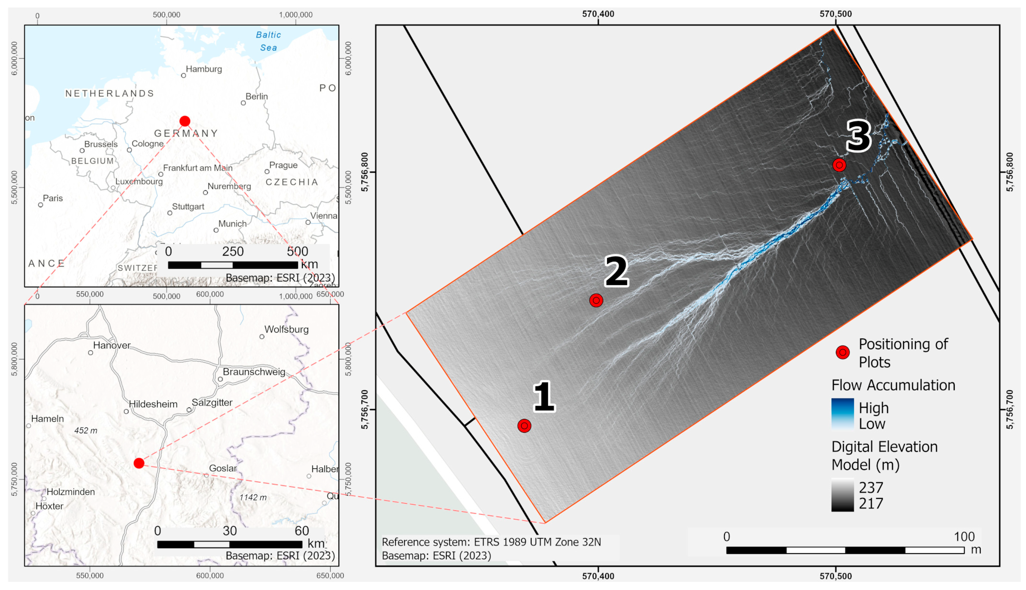
2.1.1. Study Site

The study area is located in the southern part of the German federal state Lower Saxony, near the village of Lamspringe (Figure 2). The area under investigation is situated on cropland, which is, since the year 2000, part of a long-term soil erosion monitoring program [20]. The region is characterized by a slightly hilly landscape; therefore, the height ranges from 217 to 237 m above sea level with slope gradients between 5 and 14 degrees at the study site. The predominant soil type is shallow stagnic Luvisol. Mean annual precipitation is 795 mm [21], which is in line with the average for Germany. This is also the case for the mean yearly erosivity (R-factor of the Universal Soil Loss Equation USLE [22]) between 2001 and 2017, which is at about 73 [N/h/yr] [23].

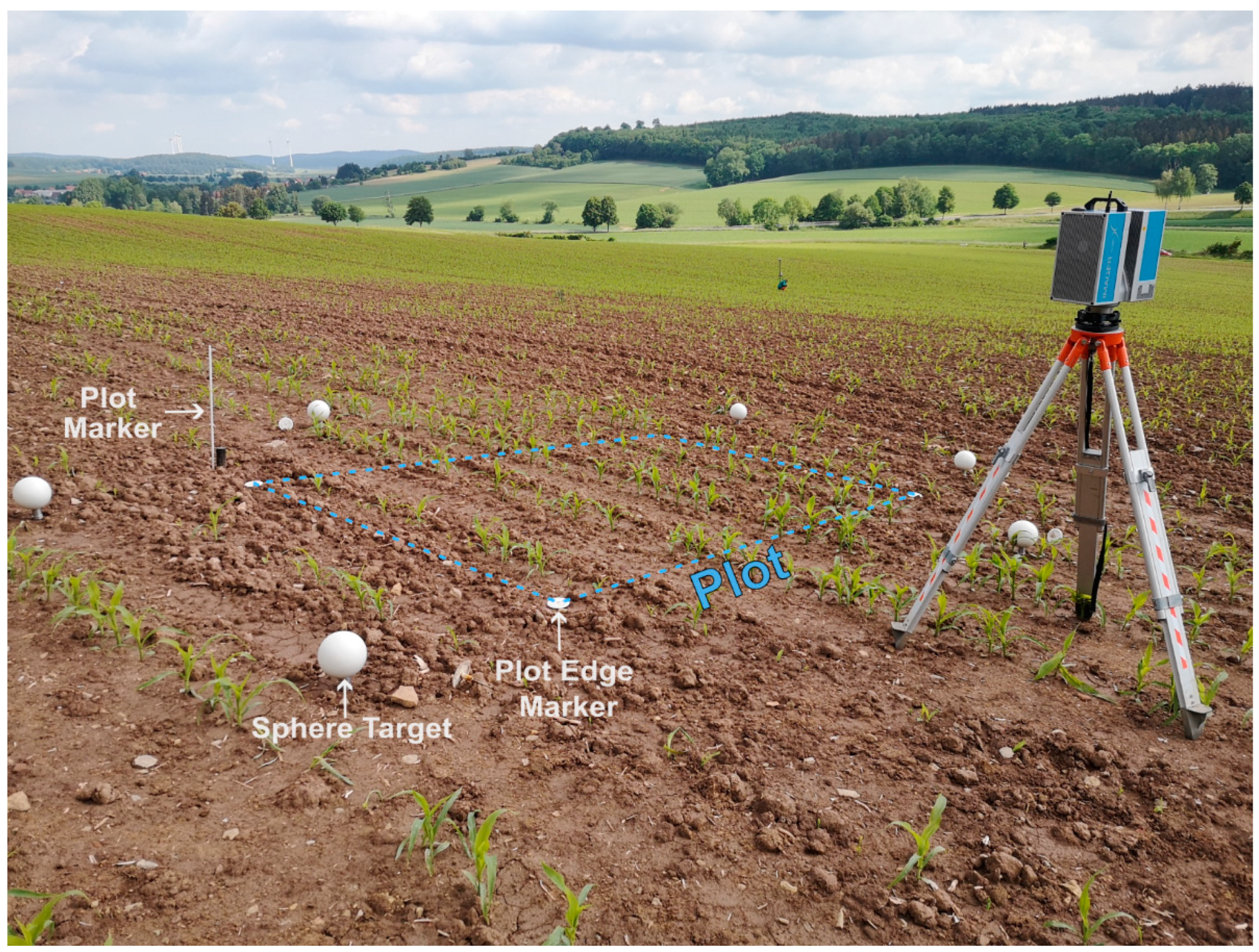
2.1.2. Field Campaign

The field campaign was conducted from 11 May 2022 to 8 June 2022, using three plots in a thalweg. The field measurements were performed on a weekly basis, starting immediately after sowing. For plot 3, the measurement started one week later. All plots covered 2 m × 3 m and were selected based on previously recorded erosion events [20] that considered different gradients in the micro-topography and slope. Specifications of the different characteristics underlying each plot are listed in Table 1. Most soil erosion events are expected to occur when low soil cover coincides with heavy rainfall occurrence. The plots were placed on cropland with late sown field crops, in this case, maize, to increase the probability that measurable erosion events accompanied by changes in the micro-relief will occur.
For each plot, a 3D point cloud was obtained weekly from two stations at a distance of about 1 m with a mean incidence angle of roughly 50 degrees. Masking of soil aggregates, tyre marks, and growing vegetation led to inhomogeneous point densities, which did not allow simple modelling via a planar surface. Growing field crops led to an increasing heterogeneity of the point density on the soil surface and a decline in the points representing the soil surface over time. The utilized laser scanner Zoller+Fröhlich (Z+F) IMAGER 5010X (scan setting with high quality, which results in approx. 0.4 points per cm2) has an integrated high dynamic range camera, providing additional RGB colour information for the 3D point cloud.
In order to set up a stable reference coordinate system, each plot was established with six control points (CP), temporarily marked with spheres (145 mm diameter) at a distance of 1 m around the plot. The measurement set-up is shown in Figure 3.
The CP positions, as well as the edges of the plot, were marked by ground sleeves driven 25 cm deep into the soil. The ground sleeves remained in the soil during the entire field campaign, whereas the spheres were removed after each measurement epoch to avoid interference with the agricultural cultivation procedures. The absolute positions of the CP were observed by determining coordinates before the weekly data acquisition procedure with a Trimble R8s GNSS System using an RTK-positioning with respect to a close-by SAPOS reference station and a measurement duration of 3 min per CP. The relatively high measurement duration allows obtaining a higher quality of reference coordinates for the subsequent registration of the point clouds.
In the following chapters, the data processing steps following the data acquisition in the field are described in detail. A first overview of the data processing is given in the workflow in Figure 4.

2.2. Data Processing

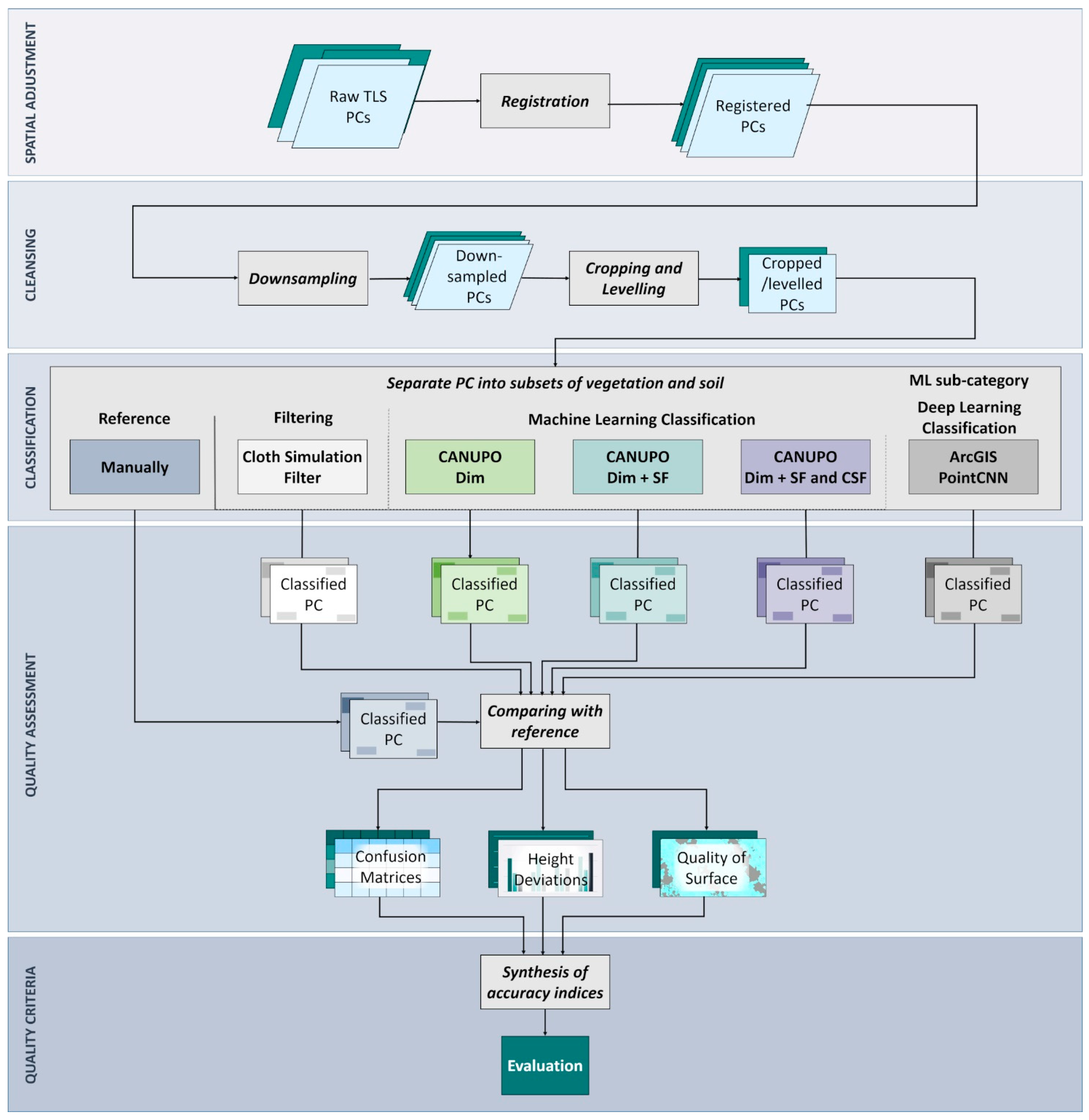
2.2.1. Spatial Adjustment and Cleansing of Point Clouds

In order to test the performance of different classification methods in our setting, we conducted the following procedure using the software Z+F LaserControl for the registration of the point clouds and the open-source software CloudCompare (version 2.12 beta), as well as the software ArcGIS Pro (2.9) for the subsequent steps.
Based on the coordinates, a target-based registration was carried out using the sphere targets (shown in Figure 3). After registration of the two 3D point clouds of the same plot across all epochs, the plot-based point clouds were downsampled using voxel grid filtering with a voxel size of 1 mm, i.e., the downsampled point clouds have an average point spacing of 1 mm [24]. This step aims for a better handling of the data and for reducing outliers and noise.
In order to further optimize data handling, the point clouds were cropped to cut the point clouds to the plot size as the area of interest.
Height differences due to a general inclination of the terrain can cause inaccuracies when using filters (resp. classificators), especially when the algorithm operates with geometrical information. Since the area under investigation has a small size, there are no large slope deviations within the plot. This simplifies the levelling of the point cloud into a horizontal position by transforming the local coordinates. Assuming a uniform tilt, the points were converted by the difference to the horizontal plane. The processed point cloud can be transformed back into the original position after processing.

2.2.2. Vegetation Detection

As the measurements were taken under field conditions, disturbing objects, like vegetation, had to be eliminated to obtain a “clean” representation of the soil surface. This is equivalent to a binary classification problem, separating points in the point clouds into soil and vegetation. Long-term soil cover as stones, as well as mulch and other plant residues, were considered to be part of the soil surface. The epoch-wise data acquisition scheme allows for a spatio-temporal analysis. One of the challenges are changing disturbing objects, e.g., growing vegetation, which may lead to varying shadowing effects on the soil surface.
As the problem of objects covering surface information occurs commonly, many algorithms to create subsets of point clouds have been developed or modified [25,26,27,28]. In this study, we used the methods CSF [17] and CANUPO (CAractérisation de NUages de POints) [18], implemented in the open-source software CloudCompare (V2.12.beta), as well as PointCNN [19] integrated as an extension of the software ArcGIS Pro (2.9).
The geometrical filter CSF computes a horizontal “cloth” grid covering the inverted point cloud surface. The point cloud and cloth grid are projected to a horizontal plane, and the nearest corresponding point of the point cloud to each of the next cloth nodes (interconnection points of the cloth, describing the structure of the cloth) is captured. Afterwards, the filter algorithm compares the distance of the original point cloud to the computed surface and separates the points into ground and non-ground points based on a threshold. For further information, please refer to [17].
In contrast to CSF, the CANUPO algorithm uses three dimensions and compares the spatial relationship of each point in the point cloud to its adjacent points at multiple scales. The number of scales, taking into account as diameters around each point, is one of the variable input settings (see Figure 1, region-based methods).
As a result, structures are identifiable that are only recognizable by referring points to the positions of their neighbourhood, in our case, elongated structured vegetation and the smoother soil surface. In its basic implementation, CANUPO considers dimensionality as a classification parameter, but there is also the option to include scalar fields as additional parameters [18]. In this study, we integrated the RGB values acquired during the TLS scanning process into the data processing steps. For this purpose, the RGB values are converted into scalar fields (SF) using the combination of the three colour bands. The intention for using this additional data is to increase the separability between living vegetation and mulch residues with similar dimensionalities but different colouring.
To achieve better results, CANUPO, including dimensionality and RGB-based scalar fields, is carried out by using CSF afterwards, as CSF is very useful in correcting outliers in the Z-direction.
As an easy-to-use representative of deep learning approaches, we also tested PointCNN implemented in ArcGIS Pro (2.9). This extension uses a generalized principle of Convolutional Neural Networks (CNN) [29]. The point cloud is first divided into blocks of a specific number of points, which are then included in the model training (see Figure 1, graph-based methods). Basically, the algorithm restructures the dense point cloud hierarchically based on local correlations of point features (e.g., RGB values, intensity) [30].
The X-Conv operator aggregates information of neighbouring points in local regions into representative points with an increased number of channels, comprising therefore more information per point. More information on the application of CNN specifically for point cloud classification can be found in [19].
After pre-testing different settings, the input parameters, which led to the best results, were finally adopted in each case. We manually selected the training and validation datasets proportionally according to class distribution across the point cloud. The ratios which produced the best results during the test phase, were used in this study (see Table 2). Training and validation data, as well as training and testing data, covered different areas of the point cloud. The different classification approaches that were tested and the initial parameter settings are listed in Table 2.

2.2.3. Quality Assessment

In order to obtain a reference for the different partitioned point cloud results, manually cleaned point clouds were generated using cropping tools of the software CloudCompare (V2.12.beta) to separate vegetation points from soil surface information. All manually cleaned results were compared with the generated reference point cloud representing the soil surface. As litter is considered part of the soil, the top layer with mulch residues was assigned to the soil surface even though mulch has a high structural similarity with living vegetation and may influence the results.
Thus, a confusion matrix [31] could be generated comparing points falsely classified as soil with points falsely classified as part of the vegetation. The focus of the evaluation lies on the accuracy in capturing vegetation; therefore, the confusion matrix represents a true positive (TP) as vegetation points correctly eliminated, a false negative (FN) as leftover vegetation, a false positive (FP) as soil being eliminated, and a true negative (TN) as correctly not-filtered points representing soil surface.
As the last step, we calculated the F1 score [32] (Equation (1)) as a harmonized mean of precision and recall. Precision depicts the proportion of positives classified (Equation (2)), while recall measures the relation of true positives to all actual positives (Equation (3)). If both precision and recall are equally high, the F1 score, ranking between 0 and 1, is high as well. Hence, an F1 score of 0.5 could be interpreted as moderate, considering the balance between precision and recall.
F 1   score = 2 Precision   ×   Recall   Precision + Recall
Precision = TP TP + FP
Recall = TP TP +   FN
As our data were highly imbalanced, we also used the balanced accuracy as a further comparable quality indicator. Balanced accuracy [33] (Equation (4)) considers the prevalence of the class and therefore recall (Equation (3)) and selectivity are used in the equation. Selectivity calculates the relation of true negatives to all actual negatives (Equation (5)). Balanced accuracy also ranges from 0 to 1, with 1 standing for the best possible classifier. A balanced accuracy of 0.5 could be interpreted as a random guess.
Balanced   Accuracy = Recall + Selectivity 2
Selectivity = TN TN + FP

3. Results

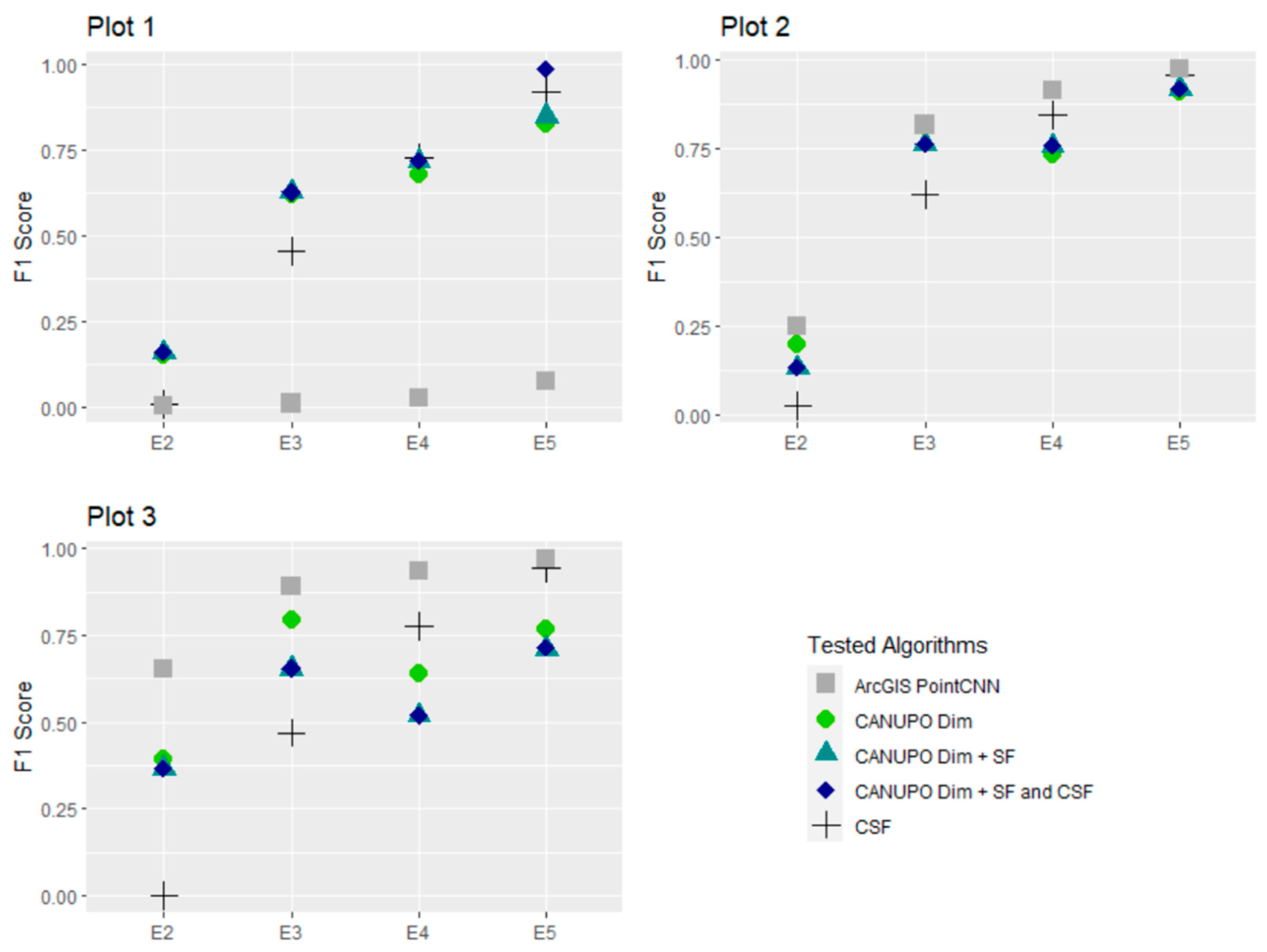
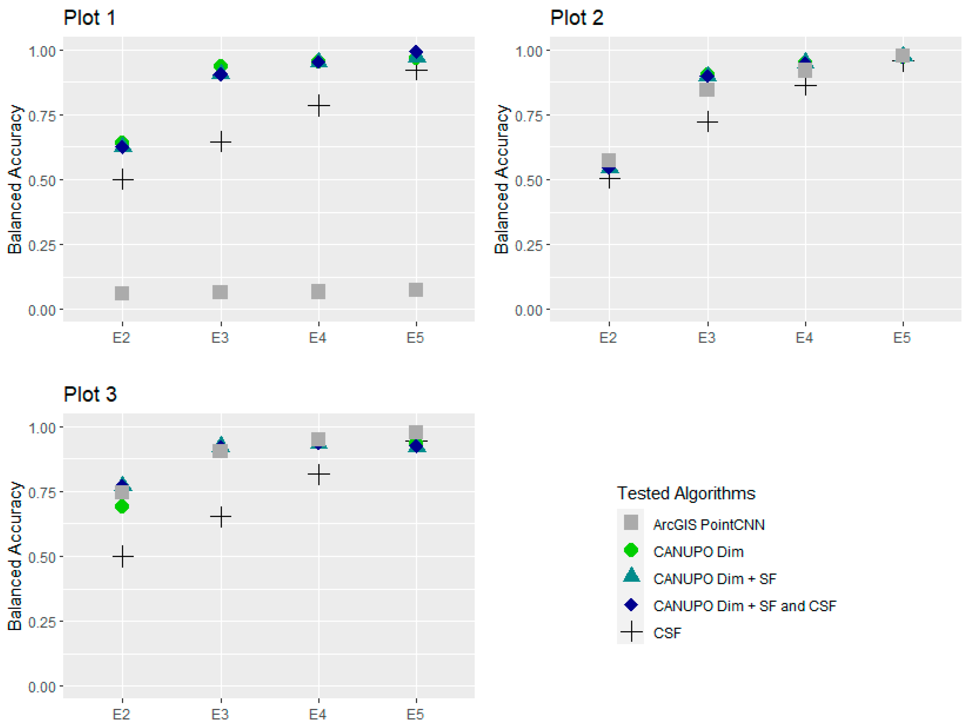
3.1. Accuracy Assessment

The described methods were implemented for all three plots of the field campaign. As stated earlier, the focus of the study lies on applicability and time saving capacity. Thus, the training data for CANUPO variations and ArcGIS Pro PointCNN was composed of all epochs for each plot, knowing that individual calculations would produce more accurate results. Afterwards, the generated classifiers were applied to each epoch of each plot separately.
To obtain an idea of the baseline data, first, the result of the manually generated reference data is shown in Table 3.
During the field campaign, the proportion of the vegetation points in the total point cloud increased exponentially, up to 15.34% in plot 3. Data gaps in the soil surface due to shadowing by vegetation become apparent in the decrease in point clouds representing the soil surface, especially in E5 for all plots. For further comparison of the algorithm performances in the different plots, it must be considered that the data acquisition in plot 3 started one week later. Since there is no vegetation in E1, this epoch is not considered in the direct comparison of the algorithm performance in vegetation detecting, but since training comprised all epochs, it could have an influence on the performance in the subsequent epochs.
The comparison of the F1 score (0 stands for either recall or precisionare of the value 0 as well, and 1 shows high matches for both precision and recall) for each tested algorithm depicts an increase with the proceeding of the timeline (Figure 5). The highest F1 scores are consistently achieved in E5 with median values over the different algorithms of 0.85, 0.92, and 0.77 for plots 1, 2, and 3, respectively. Most of the tested variations show F1 scores above 0.9 for E5, punctuating the very good performance in the scene with the highest vegetation. Accordingly, the lowest values are obtained for the epoch with the first germination with a sharp increase in the F1 score afterwards. In E2, median values for the plots are 0.15, 0.13, and 0.37, which means severely insufficient performance, presumably because of low height and structure differences that could be used for differentiation between mulch and living vegetation, for example. CSF, as a filtering tool based on height, turns out to be the one with the highest differences during the timeline because of the increasing number of points above the calculated cloth. Apart from this, caution must be exercised when directly comparing the F1 scores with CSF. Since CSF is based on height differentiation, there are no parts of the plot that are falsely categorized as vegetation (false positive). This automatically sets the precision value to 1.0 and accordingly increases the influence of recall in the F1 score. Nonetheless, comparing the tested classifications, the ArcGIS PointCNN algorithm shows the highest score for all epochs of Plots 2 and 3. Interestingly, the performance for plot 1 falls sharply out of line. Most differences between the classifications appear in plot 3, which could not only be the consequence of missing data from E1 for the training but also a different soil structure because the lower slope area, where plot 3 was located, had more stone content. Apart from E2, the overall performance for all tested algorithms—except CSF and ArcGIS PointCNN for plot 1—is satisfactory when considering the F1 score.
The balanced accuracy reveals a slightly different picture of the performance of the partitioning algorithms (Figure 6). With the balanced accuracy, the performance indicator of the used tools is cleared of the class imbalance naturally contained in the data and therefore can be considered as a more reliable performance indicator. In Figure 6, the increasing trend of the performance indicator corresponding to growing vegetation also turns up, but with a lower gradient curve. The difference in the performances between E2 and E3 is lower than in Figure 5 but is still striking. This shows that, apart from the corrected imbalance, the vegetation points in E2 are still comparably poorly recognized. For E2, only the median value for plot 3 with 0.74 can be considered to have a good performance, while plots 1 and 2 show median values of 0.63 and 0.54 and therefore moderate to unsatisfying results. Despite the low performance of ArcGIS PointCNN at Plot 1, all balanced accuracy values are located above 0.5, considering the quantity of the two classes. However, apparently, CSF shows lower performances for all plots and epochs with a median value of 0.76 and a direct dependency on vegetation height/ground cover, as the correlation with the timeline shows. As already mentioned above, false positive points are missing in CSF, which limits a direct comparison, as changes in balanced accuracy are solely based on changing recall values. In contrast to the F1 Score, ArcGIS PointCNN does not seem to have the highest rating in plots 2 and 3 for the balanced accuracy. The overall median is 0.79 (0.91 excluding Plot 3 performance), whereas the CANUPO variations all reveal an overall balanced accuracy median of 0.92 to 0.93.
Since we focused on changes in the soil microstructure using the classified point clouds, beyond the general evaluation indicators, the spatial distribution of falsely classified points and point subsets are of interest. Figure 7 shows as an example distribution of the point separation variables for the three different tested segmentation approaches on plot 2 in E2 and E5. For CANUPO, the best performing stand-alone variation with the inclusion of dimensionality and scalar field, without further usage of CSF, is shown.
Figure 7 reveals that no parts of the plot are falsely categorized as vegetation (false positive) because of the filtering method itself. This leads automatically to precision values of 1.0. Furthermore, Figure 7 shows that the seedbeds, in particular, are a problem, especially for CSF but also for all tested algorithms, as the seedbeds lie below the general soil surface. This becomes especially evident in E2, where the field crop is just sprouting, almost no true positive subsets are detected, and a recall of 0.0 is calculated. In contrast to CSF, the machine learning classification CANUPO has a higher rate of true positives in E2 and E5 but also a higher percentage of false positive parts, where soil is classified as vegetation. ArcGIS PointCNN also shows some false positive subsets, but altogether a lower falsely classified rate. In general, false positives appear mainly in E5 for CANUPO variations near the points representing crop. The higher false positive rates become obvious in the precision rates listed in Table 4. While the very high mean precision rate (1.0) of CSF shows that no false positives were detected, because of the filtering method itself, and only the low recall values contribute to an overall deficient F1 score, the CANUPO variations come off with the lowest precision values for all tested variations. Apart from that, of all points that should be classified as vegetation, CANUPO shows a solid hit rate, with a better performance when more variables are used. Nonetheless, despite the extremely low rates on Plot 1, ArcGIS PointCNN reveals the best scores both for precision and recall. The increasing trend of recall with increasing epoch can also be interpreted as a side effect of the increased hit probability with growing vegetation.

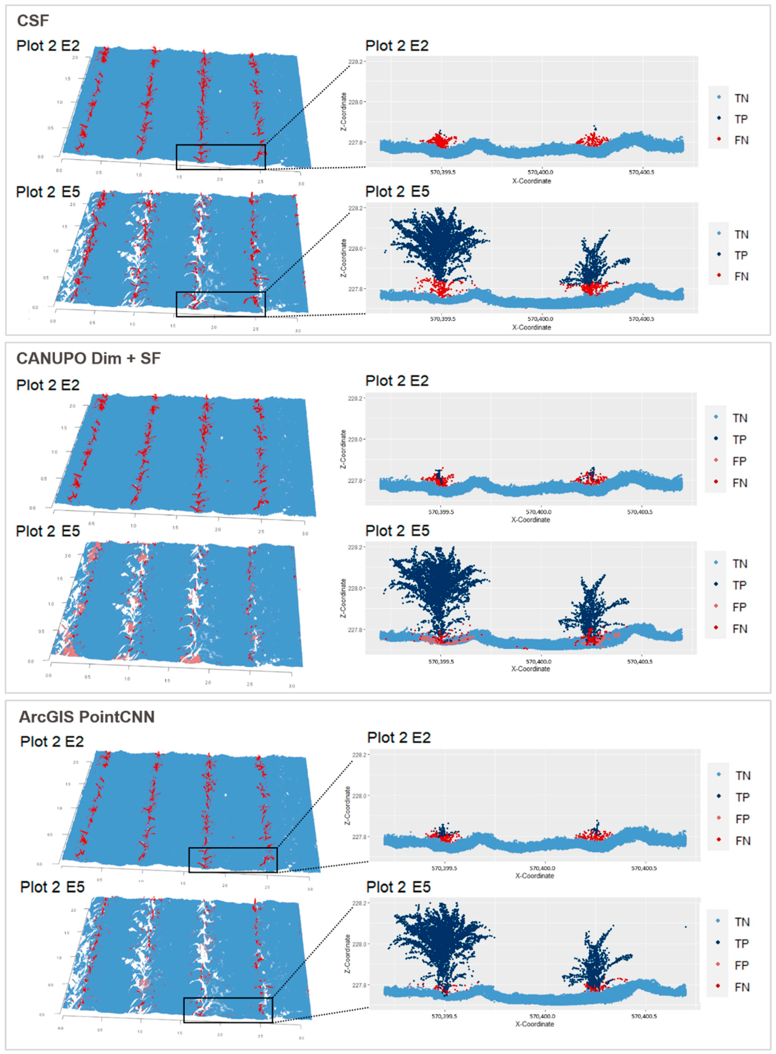
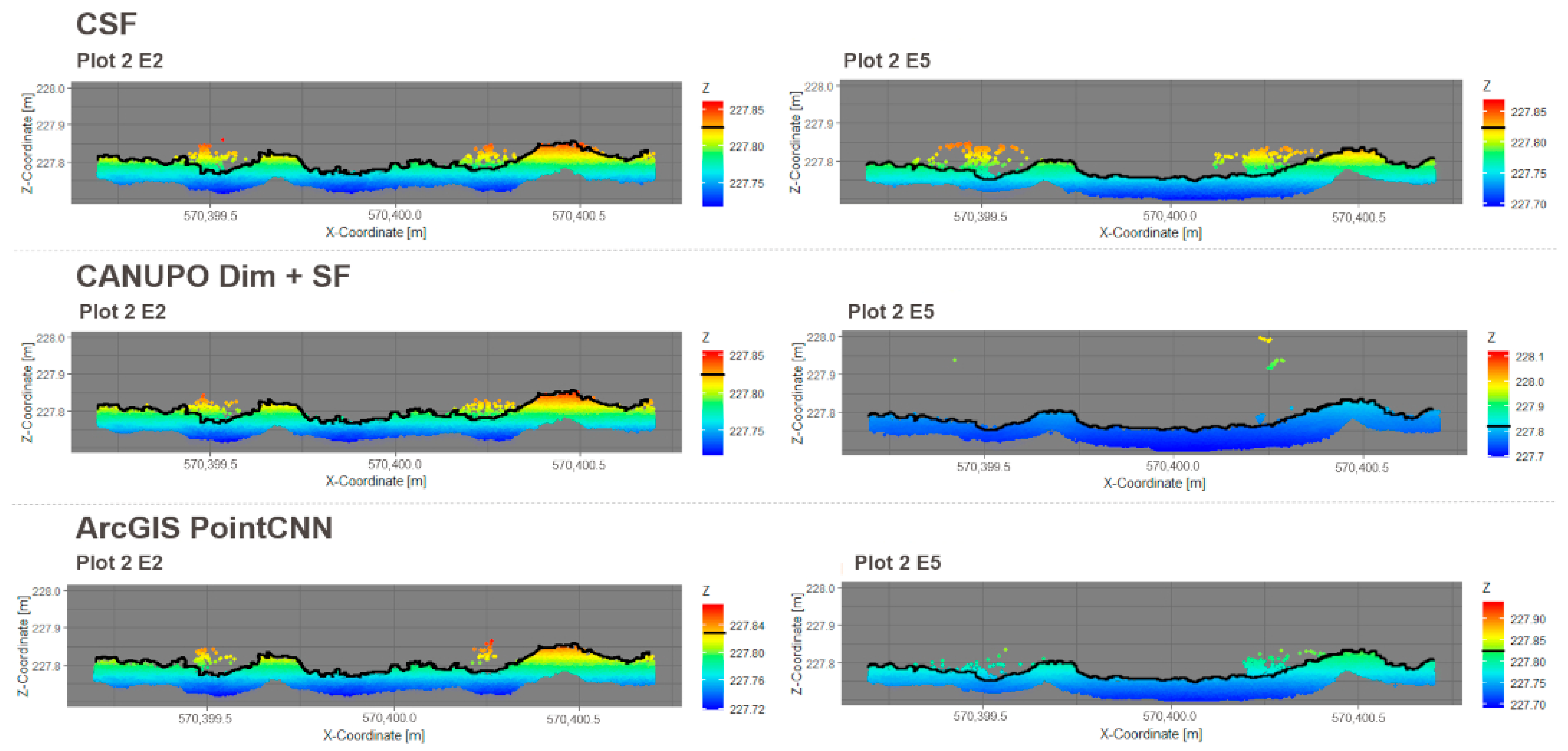
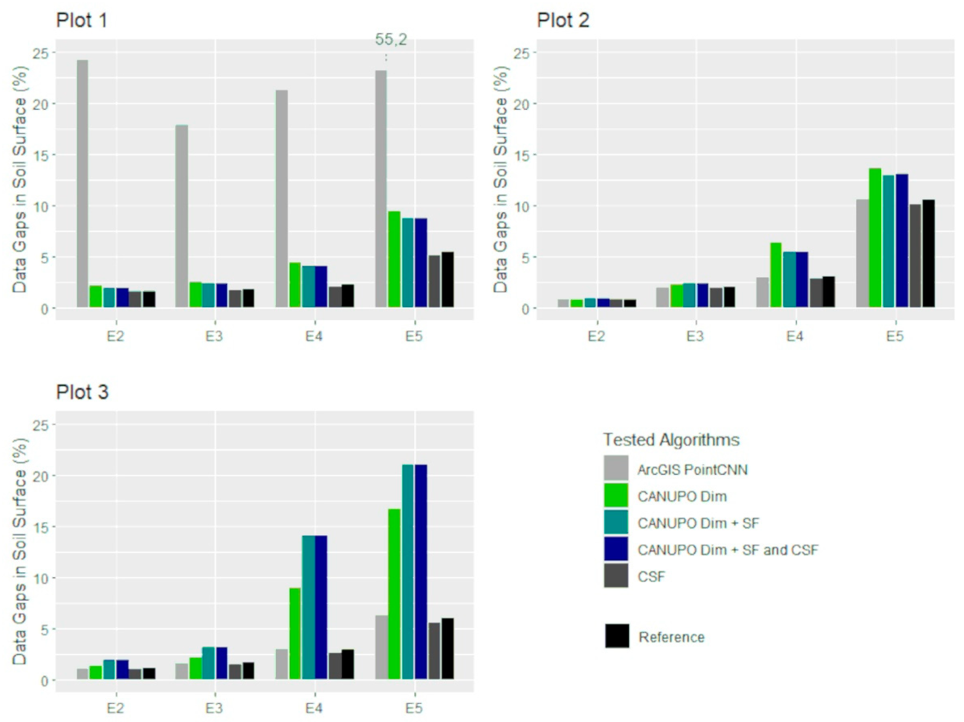
3.2. Effects of Algorithms on Soil Surface Detection

In conclusion, the characteristic values listed above show, despite the strong outliers of plot 1, a tendency in favour of the deep learning approach (PointCNN) and similar results generated from different CANUPO variations. However, the main subject of the evaluation should clearly be its effects on soil surface detection. The choice of algorithm has an impact on subsequent calculations and conclusions about soil surface changes.
As one factor correlating with soil erosion detection, the following section focuses on height differences but also the changes in the underlying data quality arising from algorithm choice. Table 5 gives an overview of the average surface height differences in comparison with the corresponding reference surface and standard deviations (SD) of the height difference calculations compared to the reference soil surface. While CSF shows, in general (with the exception of ArcGIS PointCNN variation in plot 1 with 2.4 mm), the highest mean height deviations in comparison to the reference surface (0.1–0.8 mm), the lowest average height deviations arise with the usage of CANUPO variations (0.0–0.5 mm). Results of ArcGIS PointCNN are comparable except for plot 1. The more interesting aspect seems to be the standard deviation of the discrepancy between the height values of the surfaces cleaned by an algorithm and the manually created reference surface. The best values are produced with the combination of CANUPO and CSF (SD: 0.8–1.5 mm). The ArcGIS PointCNN application stands out because it has comparatively high standard deviations but low average height deviations. Despite the results of ArcGIS PointCNN for plot 1, the height differences are not significant but can still give clues to the performance of the algorithms.
The exemplary cross-sections of plot 2 with the absolute Z-coordinates (shown in Figure 8) reveal the functioning of the different filtering and classification tools. The simple filtering of points due to their relative height values results in a surface without any strong outliers. The range of the Z-coordinates stays similar regardless of the proceeding epoch. Hence, the increasing height differences to the reference arise from the growing vegetation between E2 and E4. The highest range difference to the reference surface shows the CANUPO variation with the integration of scalar field information. The difference in the highest points reaches up to 90 cm in the displayed subsection of plot 2, E5. Nonetheless, most of the outliers can be corrected using CSF afterwards (CANUPO Dim + SF and CSF, not shown in Figure 8). Overall, the crop is captured quite well vertically with CANUPO. The problem with single outliers also exists when using ArcGIS PointCNN, as can be seen in the deviating range of plot 2, E5 in Figure 8.
The comparison of height structure as a result of point cloud segmentation shows that CANUPO has a solid hit rate but a slightly lower standard deviation due to the deep learning approach. However, another factor affecting data quality when comparing soil structure changes over time is the data availability in the horizontal direction. As a result of data acquisition over a time period of six weeks, the quality of the reference data itself is subject to variability. As stated before, the growing of the field crop leads to increasing shadowing with the resulting expansion of parts in the soil surface with no data availability. These data gaps in the reference soil surface range from 0.8% (plot 2 E2) to 10.6% (plot 2 E5). Depending on the classification process used, the gaps where no data is provided for surface structure analysis alternates. Figure 9 relates the number and size of data gaps depending on the tested algorithms relative to each other. In plot 1, ArcGIS PointCNN shows very high divergences in all four epochs, with the result of more than half of the soil surface (55.2%) being deleted in E5. Despite that outcome, not only does the trend of increasing data gaps with the proceeding time step crystallize strongly but also the increase in data gaps due to growing vegetation in subsequent epochs. While CSF shows slightly lower percentages of no data parts in the horizontal direction than the reference surface, the CANUPO variations produce bigger holes in the soil surface with ranges from 0.8% (plot 2 E2 CANUPO Dim) to 21.1% (plot 3 E5 CANUPO Dim + SF and CSF). This is concurrent with the extracted high counts of FN points for CSF, respectively; high counts for FP points for CANUPO variations (see Section 3.1). Detection of vegetation seems to be the biggest challenge in plot 3. Comparing the data gaps, the fact that the bare surface of E1 is missing in the training data in plot 3 becomes evident. Apparently, the bare soil surface as reference is very important for the training of the CANUPO classifier, as (apart from ArcGIS Point CNN of plot 1) the highest gaps appear in E4 and E5 of plot 3. As the combination with RGB values (CANUPO Dim + SF and CANUPO Dim + SF and CSF) especially stands out, the colour of soil, which changes in the course of the weekly measurements depending on the soil moisture, in E1 could be of importance. Furthermore, since the shadowing of vegetation leads to data gaps in the reference soil surface, the reference of the bare ground in E1 below the vegetation can influence the region-growing model.

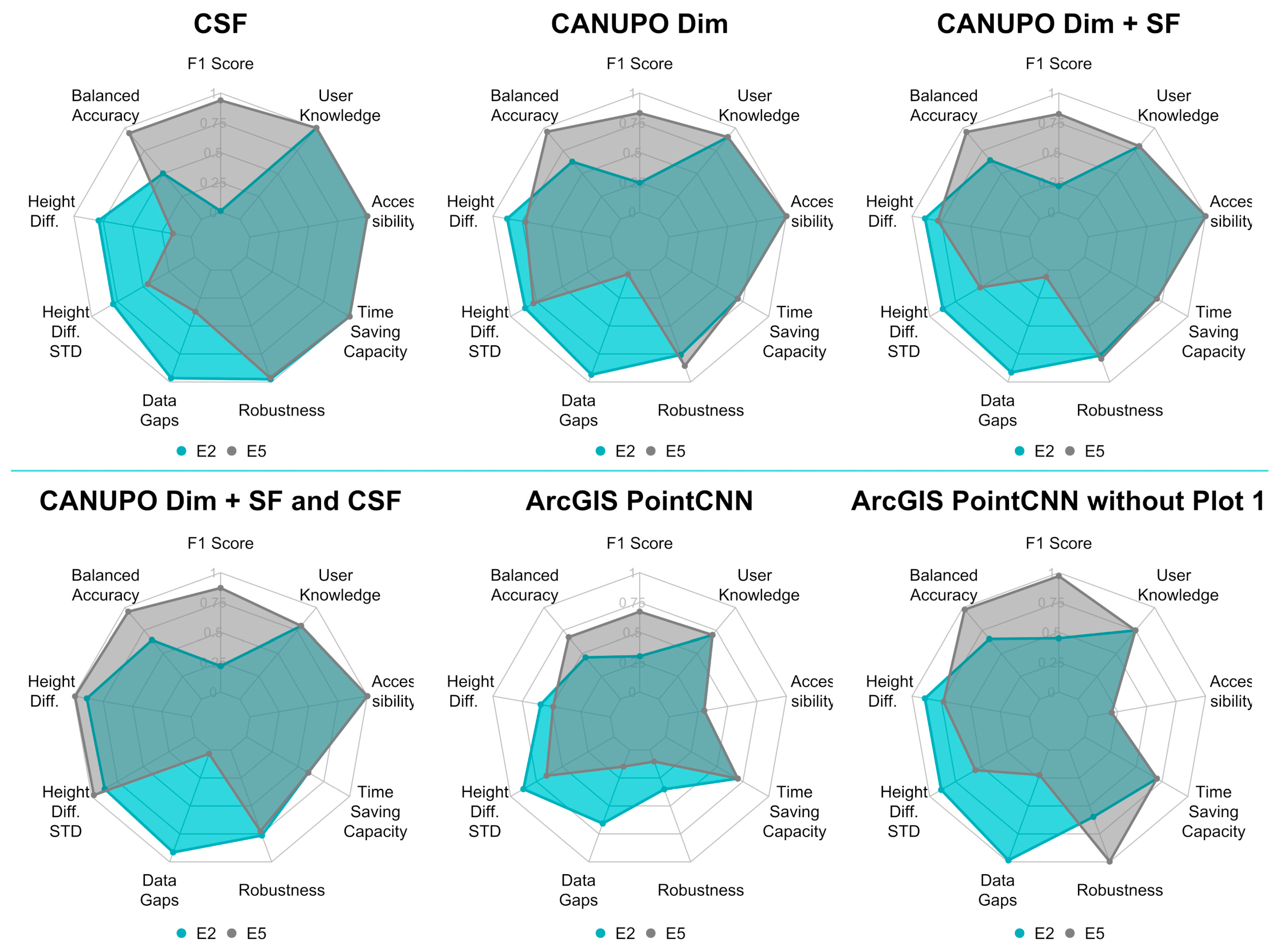
3.3. Quality Criteria for Evaluation of the Tested Algorithms

In this section, we look at the question of which algorithm under investigation is the best choice for point clouds at the microscale. On top of the performance indicators and the quality differences in the resulting datasets as hard assessment criteria, the handling of the different algorithms is also included as soft evaluation criteria. For this purpose, we transferred the calculated values listed above into the rating scheme 0 to 1, with 1 being the best-derived value. Furthermore, the ranges of the F1 scores for the three different plots of the same epoch were compared and transferred to the rating scheme 0 to 1, with 1 being the lowest derived difference. These criteria show the robustness of the results and can be interpreted as the sensitivity to the variability of input data. The criteria describing the handling of the algorithms is denoted as soft evaluation criteria as there are no hard values behind the evaluation. They describe the personal perception regarding the applicability of the algorithms. In Table 6, the used criteria and their derivation are listed. Since the temporal aspect also plays a role, E2 and E5 were presented separately as extremes in the time span.
Figure 10 shows the combination of all evaluation criteria, considered useful for the process of algorithm choice in the research setting of microscale point cloud segmentation. As expected, easier handling comes along with lower performance, as with the usage of CSF. Contrary to this, the more time-intensive combination of CANUPO applications with CSF leads to higher performance indices in E5. This seems to be unappealing to E2, as we can already see in the subchapters above. The deep learning application (ArcGIS PointCNN) had problems with the detection of vegetation in plot 1. The influence of the results of plot 1 caused a low rating for all hard evaluation criteria, with a particularly low robustness value. For a better comparison, the evaluation of ArcGIS PointCNN without plot 1 is also shown in Figure 10, which shows similar values when plot 1 is not considered. Apart from this, this algorithm stands out due to low values representing the handling of the tool. Additionally, machine learning applications in ArcGIS Pro are relatively new extensions that have to be installed on top of the basic ArcGIS Pro application. As ArcGIS Pro itself is a licensed product from ESRI, the accessibility of ArcGIS PointCNN is limited. As a consequence of the relative novelty of the machine learning extensions and limited access, the community of users is still small. This influences the needed prior user knowledge, as the open-source software CloudCompare gives far more possibilities for self-learning. Altogether, this leads to a lower evaluation value for the categories of user knowledge, accessibility and time saving capacity. Apart from the results of plot 1, the ArcGIS PointCNN algorithm from ESRI had an outstanding performance (Figure 10), but even with the high-performance values of plots 2 and 3, the low accessibility should be taken into consideration before choosing this algorithm.
Another conclusion that can be drawn from Figure 10 is the different performance of all algorithms in relation to the growth stage of the crop. Obviously, the two aspects, namely good detection of vegetation and a high percentage of data representing the soil surface, are divergent. Further investigations might help find the timing with the sweet spot of both opposing components.

4. Discussion

The accuracy of the data representing the soil surface does not only depend on the resolution of the sensing devices but also on the precision of the succeeding detection/filtering methods. When it comes to capturing small changes in the soil surface especially, the performance of the used data filtering or classification method is crucial.
During data acquisition in a time period of six weeks in our study, the local reference coordinate system was kept as stable as possible to maintain comparability between epochs of data measurement. As the targets were set up directly in soils under cultivation, internal physical processes (e.g., swelling and shrinking of soil aggregates) or external influences (e.g., soil tillage) led to the movement of the targets, resulting in standard deviations of 3.6 mm of the target positions in the z-axis. Focusing on changes at the microscale may have influenced the training of the classifier, as all of the training data contained all epochs.
Shading and masking of growing vegetation increased with the duration of the measurement campaign. The consequences are, on the one hand, accumulative gaps in the point cloud representing the soil surface and, on the other hand, an increase in undesirable data which derives from crop growth. Despite that issue, this set-up has the advantage that we only need to distinguish (roughly speaking) between (a) points representing vegetation and (b) points representing soil. Thus, we can use well-established filtering and classification algorithms with the binary classification approach.
Although there are plenty of studies dealing with the performances of filtering or classification algorithms, most of them are predominantly geared towards larger scales [13,34,35] or focus on applications that require programming skills [12,30,36]. Bailey et al. (2022) [37] demonstrate in their study that the performance of the different algorithms highly depends on the parameter settings. In their study, CSF outperforms Random Forest (RF) and modified slope-based filter (MSBF). The change in the parameter settings in CSF did not improve the results in our case. One explanation could be mulch residues, which, in our study, were assigned to the soil surface and had a strong influence on the performance of all tested applications. While the higher epochs almost consistently show good results, even in comparison with other studies [13,37], two noticeable issues arise:
Firstly, ArcGIS PointCNN did not work out in classifying plot 1. Although the amount of training data was similar to the training data of the other plots, ArcGIS PointCNN performed much better in the point clouds of the other plots. The results of all epochs in plot 1 for this algorithm indicate that there must have been a problem with the training data. Even though changes in the training data amount did not particularly improve the results, we plan to conduct more experiments (using evenly distributed training data and training data for each epoch separately). One assumption is that the “generalization gap” phenomenon occurred in this plot [38]. The generalization gap is a phenomenon that sometimes occurs when supervised deep learning methods and high training data accuracy are used. When overfitting occurs, the trained function performs well on the training data but also becomes sensitive towards noise, following up with a low performance on the actual data and therefore producing a generalization error [39,40]. As our data are highly dense, the noise of the data certainly contributes to model irritations. The use of the k-fold cross-validation could have helped to prevent this problem, as it predicts the performance of models based on predefined training data [41,42].
Secondly, there is a visible variability of the performance depending on the plot as a starting point and a high variability depending on the epoch. Altogether, the algorithms show lower quality in plot 3. As the E1 reference in the training data is missing, this reveals the importance of the bare soil surface data. The region-growing model of the CANUPO classifier especially depends on the information below vegetation, as data gaps in the training data can apparently cause irritations in the model. This leads to the question of whether a less voxel-grid filtered point cloud could provide better results in the utilization of the CANUPO algorithm. Furthermore, as soil colour changes, depending on the soil moisture, the darker colour at the beginning of the field campaign could have supported a better differentiation of soil and vegetation in the training of CANUPO for plots 1 and 2. The missing E1 data did not affect ArcGIS PointCNN. This could be explained by the underlying method of the algorithm. As this algorithm is not a region-based model (Figure 1) but a graph-based model, it also includes further information on the different points, and the influence of neighbouring is decreased. This also shows the importance of aligning the method with the underlying data. In this respect, the different soil surface structures of the different plots also influence the outcome of the modelling. As plot 3 is located on the lower part of the slope, it is characterized by a higher coverage of stones and mulch. The similarity of mulch and living vegetation is a problem, which also shows off in the other plots but could sum up with increasing coverage.
Furthermore, this could be the explanation for the low performance of all applications on epoch 2 as well. The small proportion of living vegetation in epoch 2 and the still low contrasting colour of the seedlings only offer a small basis for differentiation.

5. Conclusions

We approached the assessment of three main point cloud classification concepts (filtering, machine learning classification not based on deep neuronal networks, and deep learning classification as a machine learning sub-category based on deep neuronal networks) from different angles. The standard procedure is first presented with the F1 score, which shows the harmonized mean of precision and recall. Since we have highly imbalanced data, we also focused on balanced accuracy as a further quality indicator. Both indicators display the quality of the overall performance of the tested algorithms. As a next step, depending on the focus of the underlying scientific question, such as the detection of diffuse soil erosion, the vertical and horizontal structure of the resulting surface is compared to the best possible outcome. As this is of probable interest to other scientists dealing with similar questions, these findings are also presented in a chapter of its own.
Based on these results, we then created a synthesis comparing the quality criteria to evaluate which algorithm under investigation is the best choice for point clouds at the microscale.
Overall, the research questions can be answered as follows:
(1)
Can well-known methods provide sufficiently accurate results in separating vegetation from soil at the plot scale?
This question cannot be answered positively without reservation.
Focusing on epochs 3 to 5, the easy-to-use and open-source method CANUPO, with the usage of colour as a scalar field and in combination with CSF, performs exceptionally well. Outliers remaining after the use of CANUPO can be well eliminated with CSF. When a high imbalance in the distribution of the classes occurs, as in epoch 2, ArcGIS PointCNN is a better choice. However, it should be considered that, depending on the algorithm, there is more loss of the soil surface, resulting in data gaps (CANUPO) or more undesirable data remaining in the final product (CSF).
(2)
Can these algorithms maintain their level of accuracy at different epochs during the examined vegetation growing period and different plots?
None of the tested methods could maintain their level of accuracy at different epochs and plots. The highest differences appeared between epoch 2 and epoch 3 for all tested algorithms. So, as mentioned before, care should be taken with imbalanced and noisy data at the plot scale.
(3)
To what extent does the choice of the algorithm affect the results?
When it comes to the changes in the micro-relief, differences in the centimetre to millimetre scale become important. The highest standard variation in the height values appeared after applying ArcGIS PointCNN, as it does not work with the region growing method. The resulting surface structure differed most quantitatively with CSF. With regard to the effect on the surface structure, the CANUPO variation in combination with CSF is the best choice. Nonetheless, CSF can also be applied after using ArcGIS PointCNN.
(4)
Does the complexity of the application increase the accuracy of the results?
Most of the results showed a better performance of the deep learning application ArcGIS PointCNN. However, this does not apply to plot 1. In addition to the generalization gap mentioned above, there are more shortcomings when using deep learning methods. The higher the complexity of the model, the higher the adaption to the specific situation is required. This problem is pointed out in [39], leading to the result that there is no algorithm which fits best for all situations and problems. Additionally, in order to prevent overfitting, the use of k-fold cross-validation could be of great value, as it can predict the accuracy of a training model [41,42].
In summary, there are applications that are less suitable than others when a relatively simple solution but sufficient accuracy is required. Taking into consideration the performances of the used methods but also the soft evaluation criteria (see Section 3), we would generally recommend the CANUPO variation with RGB as a scalar field in combination with CSF afterwards when easy-to-use classifications are needed. Besides this, some questions in regard to the “Epoch 2 problem” remain open and remain to be investigated.

Author Contributions

Conceptualization, S.O. and B.S.-K.; methodology, S.O.; software, S.O.; validation, S.O., B.S.-K., C.H. and J.-A.P.; formal analysis, S.O.; investigation, S.O.; resources, B.B. and J.-A.P.; data curation, S.O. and J.-A.P.; writing—original draft preparation, S.O.; writing—review and editing, S.O., C.H., J.-A.P., B.S.-K. and B.B.; visualization, S.O.; supervision, B.S.-K. and B.B.; project administration, S.O. and B.S.-K.; funding acquisition, B.S.-K. and B.B. All authors have read and agreed to the published version of the manuscript.

Funding

This research received funding from the Lower Saxonian State Authority for Mining, Energy and Geology of Lower Saxony (Landesamt für Bergbau, Energie und Geologie, LBEG), as it is a spin-off of the Lower Saxonian soil erosion monitoring programme (funding code: 207-4500125027).

Informed Consent Statement

Not applicable.

Data Availability Statement

Data are contained within the article.

Acknowledgments

Every fieldwork needs helping hands. We are thankful for the support of Alexander Störmer, Heiko van Wensen, Marc Neumann, Sarah Hilleckes, and Leonhard Pleuger.

Conflicts of Interest

The authors declare no conflict of interest.

References

  1. Wuepper, D.; Borrelli, P.; Finger, R. Countries and the global rate of soil erosion. Nat. Sustain. 2020, 3, 51–55. [Google Scholar] [CrossRef]
  2. Eekhout, J.P.C.; de Vente, J. Global impact of climate change on soil erosion and potential for adaptation through soil conservation. Earth-Sci. Rev. 2022, 226, 103921. [Google Scholar] [CrossRef]
  3. Eltner, A.; Mulsow, C.; Maas, H.-G. Quantitative measurement of soil erosion from tls and uav data. Int. Arch. Photogramm. Remote Sens. Spatial Inf. Sci. 2013, XL-1/W2, 119–124. [Google Scholar] [CrossRef]
  4. Cândido, B.M.; Quinton, J.N.; James, M.R.; Silva, M.L.N.; de Carvalho, T.S.; de Lima, W.; Beniaich, A.; Eltner, A. High-resolution monitoring of diffuse (sheet or interrill) erosion using structure-from-motion. Geoderma 2020, 375, 114477. [Google Scholar] [CrossRef]
  5. Cucchiaro, S.; Carretta, L.; Nasta, P.; Cazorzi, F.; Masin, R.; Romano, N.; Tarolli, P. Multi-temporal geomorphometric analysis to assess soil erosion under different tillage practices: A methodological case study. J. Agric. Eng. 2022, 53, 1279. [Google Scholar] [CrossRef]
  6. Pineux, N.; Lisein, J.; Swerts, G.; Bielders, C.L.; Lejeune, P.; Colinet, G.; Degré, A. Can DEM time series produced by UAV be used to quantify diffuse erosion in an agricultural watershed? Geomorphology 2017, 280, 122–136. [Google Scholar] [CrossRef]
  7. Balaguer-Puig, M.; Marqués-Mateu, Á.; Lerma, J.L.; Ibáñez-Asensio, S. Estimation of small-scale soil erosion in laboratory experiments with Structure from Motion photogrammetry. Geomorphology 2017, 295, 285–296. [Google Scholar] [CrossRef]
  8. Kaiser, A.; Erhardt, A.; Eltner, A. Addressing uncertainties in interpreting soil surface changes by multitemporal high-resolution topography data across scales. Land Degrad. Dev. 2018, 29, 2264–2277. [Google Scholar] [CrossRef]
  9. Luo, J.; Zheng, Z.; Li, T.; He, S. Changes in micro-relief during different water erosive stages of purple soil under simulated rainfall. Sci. Rep. 2018, 8, 3483. [Google Scholar] [CrossRef]
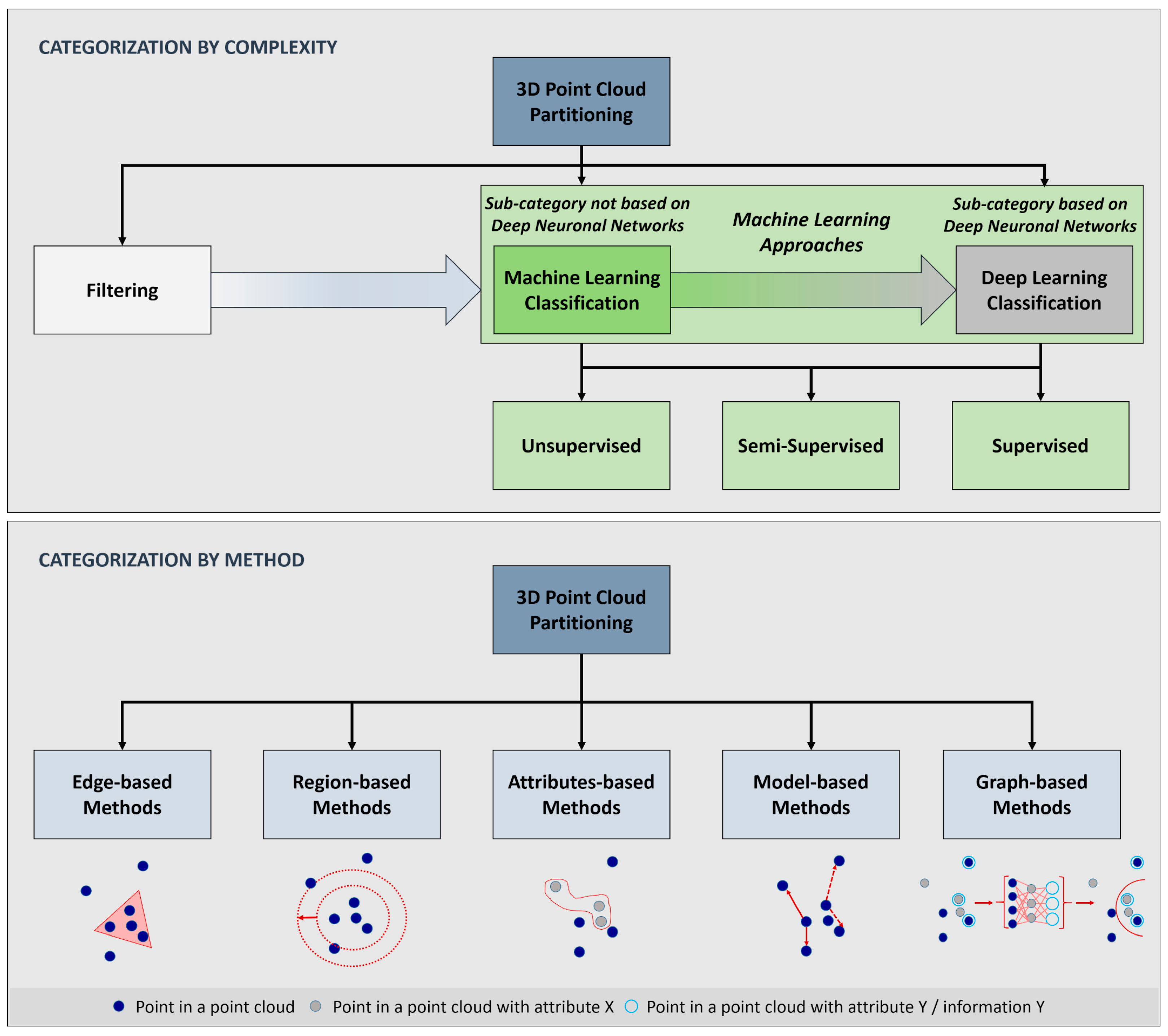
  10. Grilli, E.; Menna, F.; Remondino, F. A review of point clouds segmentation and classification algorithms. Int. Arch. Photogramm. Remote Sens. Spatial Inf. Sci. 2017, XLII-2/W3, 339–344. [Google Scholar] [CrossRef]
  11. Weinmann, M.; Schmidt, A.; Mallet, C.; Hinz, S.; Rottensteiner, F.; Jutzi, B. Contextual classification of point cloud data by exploiting individual 3d neigbourhoods. ISPRS Ann. Photogramm. Remote Sens. Spatial Inf. Sci. 2015, II-3/W4, 271–278. [Google Scholar] [CrossRef]
  12. Pinto, M.F.; Melo, A.G.; Honório, L.M.; Marcato, A.L.M.; Conceição, A.G.S.; Timotheo, A.O. Deep Learning Applied to Vegetation Identification and Removal Using Multidimensional Aerial Data. Sensors 2020, 20, 6187. [Google Scholar] [CrossRef] [PubMed]
  13. Štroner, M.; Urban, R.; Lidmila, M.; Kolář, V.; Křemen, T. Vegetation Filtering of a Steep Rugged Terrain: The Performance of Standard Algorithms and a Newly Proposed Workflow on an Example of a Railway Ledge. Remote Sens. 2021, 13, 3050. [Google Scholar] [CrossRef]
  14. Kermarrec, G.; Yang, Z.; Czerwonka-Schröder, D. Classification of Terrestrial Laser Scanner Point Clouds: A Comparison of Methods for Landslide Monitoring from Mathematical Surface Approximation. Remote Sens. 2022, 14, 5099. [Google Scholar] [CrossRef]
  15. Nguyen, A.; Le, B. 3D point cloud segmentation: A survey. In Proceedings of the 2013 6th IEEE Conference on Robotics, Automation and Mechatronics (RAM), Manila, Philippines, 12–15 November 2013; IEEE: Piscataway, NJ, USA, 2013; pp. 225–230, ISBN 978-1-4799-1201-8. [Google Scholar]
  16. Sarker, I.H. Deep Learning: A Comprehensive Overview on Techniques, Taxonomy, Applications and Research Directions. SN Comput. Sci. 2021, 2, 420. [Google Scholar] [CrossRef]
  17. Zhang, W.; Qi, J.; Wan, P.; Wang, H.; Xie, D.; Wang, X.; Yan, G. An Easy-to-Use Airborne LiDAR Data Filtering Method Based on Cloth Simulation. Remote Sens. 2016, 8, 501. [Google Scholar] [CrossRef]
  18. Brodu, N.; Lague, D. 3D terrestrial lidar data classification of complex natural scenes using a multi-scale dimensionality criterion: Applications in geomorphology. ISPRS J. Photogramm. Remote Sens. 2012, 68, 121–134. [Google Scholar] [CrossRef]
  19. Li, Y.; Bu, R.; Sun, M.; Wu, W.; Di, X.; Chen, B. PointCNN: Convolution On X-Transformed Points. In Proceedings of the NIPS’18: Proceedings of the 32nd International Conference on Neural Information Processing Systems, Red Hook, NY, USA, 3–8 December 2018; pp. 828–838. [Google Scholar]
  20. Steinhoff-Knopp, B.; Burkhard, B. Soil erosion by water in Northern Germany: Long-term monitoring results from Lower Saxony. CATENA 2018, 165, 299–309. [Google Scholar] [CrossRef]
  21. DWD Climate Data Center (CDC). Multi-Annual Grids of Precipitation Height over Germany 1981–2010, version v1.0; Deutscher Wetterdienst (DWD): Offenbach/Main, Germany, 2018.
  22. Wischmeier, W.H.; Smith, D.D. Predicting Rainfall-Erosion Losses from Cropland East of the Rocky Mountains: Guide for Selection of Practices for Soil and Water Conservation; Agricultural Research Service, U.S. Dept. of Agriculture in cooperation with Purdue Agricultural Experiment Station: Washington, DC, USA, 1965.
  23. Fischer, F.K.; Winterrath, T.; Junghänel, T.; Walawender, E.; Auerswald, K. Mean Annual Precipitation Erosivity (R Factor) Based on RADKLIM Version 2017.002; Deutscher Wetterdienst (DWD): Offenbach/Main, Germany, 2019. [CrossRef]
  24. Rusu, R.B.; Cousins, S. 3D is here: Point Cloud Library (PCL). In Proceedings of the IEEE International Conference on Robotics and Automation (ICRA), Shanghai, China, 9–13 May 2011; IEEE: Piscataway, NJ, USA, 2011; pp. 1–4. [Google Scholar] [CrossRef]
  25. Pingel, T.J.; Clarke, K.C.; McBride, W.A. An improved simple morphological filter for the terrain classification of airborne LIDAR data. ISPRS J. Photogramm. Remote Sens. 2013, 77, 21–30. [Google Scholar] [CrossRef]
  26. Wu, Y.; Sang, M.; Wang, W. A Novel Ground Filtering Method for Point Clouds in a Forestry Area Based on Local Minimum Value and Machine Learning. Appl. Sci. 2022, 12, 9113. [Google Scholar] [CrossRef]
  27. Jia, C.C.; Wang, C.J.; Yang, T.; Fan, B.H.; He, F.G. A 3D Point Cloud Filtering Algorithm based on Surface Variation Factor Classification. Procedia Comput. Sci. 2019, 154, 54–61. [Google Scholar] [CrossRef]
  28. Ao, Z.; Wu, F.; Hu, S.; Sun, Y.; Su, Y.; Guo, Q.; Xin, Q. Automatic segmentation of stem and leaf components and individual maize plants in field terrestrial LiDAR data using convolutional neural networks. Crop J. 2022, 10, 1239–1250. [Google Scholar] [CrossRef]
  29. Li, Z.; Liu, F.; Yang, W.; Peng, S.; Zhou, J. A Survey of Convolutional Neural Networks: Analysis, Applications, and Prospects. IEEE Trans. Neural Netw. Learn. Syst. 2022, 33, 6999–7019. [Google Scholar] [CrossRef]
  30. Fareed, N.; Flores, J.P.; Das, A.K. Analysis of UAS-LiDAR Ground Points Classification in Agricultural Fields Using Traditional Algorithms and PointCNN. Remote Sens. 2023, 15, 483. [Google Scholar] [CrossRef]
  31. Ting, K.M. Confusion Matrix. In Encyclopedia of Machine Learning; Sammut, C., Webb, G.I., Eds.; Springer: Boston, MA, USA, 2010; p. 209. ISBN 978-0-387-30164-8. [Google Scholar]
  32. Zhang, E.; Zhang, Y. F-Measure. In Encyclopedia of Database Systems; Liu, L., Özsu, M.T., Eds.; Springer: Boston, MA, USA, 2009; p. 1147. ISBN 978-0-387-39940-9. [Google Scholar]
  33. Wegier, W.; Ksieniewicz, P. Application of Imbalanced Data Classification Quality Metrics as Weighting Methods of the Ensemble Data Stream Classification Algorithms. Entropy 2020, 22, 849. [Google Scholar] [CrossRef] [PubMed]
  34. Chen, C.; Guo, J.; Wu, H.; Li, Y.; Shi, B. Performance Comparison of Filtering Algorithms for High-Density Airborne LiDAR Point Clouds over Complex LandScapes. Remote Sens. 2021, 13, 2663. [Google Scholar] [CrossRef]
  35. Jayakumari, R.; Nidamanuri, R.R.; Ramiya, A.M. Object-level classification of vegetable crops in 3D LiDAR point cloud using deep learning convolutional neural networks. Precis. Agric. 2021, 22, 1617–1633. [Google Scholar] [CrossRef]
  36. Jurado, J.M.; Cárdenas, J.L.; Ogayar, C.J.; Ortega, L.; Feito, F.R. Semantic Segmentation of Natural Materials on a Point Cloud Using Spatial and Multispectral Features. Sensors 2020, 20, 2244. [Google Scholar] [CrossRef]
  37. Bailey, G.; Li, Y.; McKinney, N.; Yoder, D.; Wright, W.; Herrero, H. Comparison of Ground Point Filtering Algorithms for High-Density Point Clouds Collected by Terrestrial LiDAR. Remote Sens. 2022, 14, 4776. [Google Scholar] [CrossRef]
  38. Hoffer, E.; Hubara, I.; Soudry, D. Train longer, generalize better: Closing the generalization gap in large batch training of neural networks. Adv. Neural Inf. Process. Syst. 2017, 30, 1729–1739. [Google Scholar] [CrossRef]
  39. Wolpert, D.H. The Lack of A Priori Distinctions Between Learning Algorithms. Neural Comput. 1996, 8, 1341–1390. [Google Scholar] [CrossRef]
  40. Goodfellow, I.; Courville, A.; Bengio, Y. Deep Learning; The MIT Press: Cambridge, MA, USA, 2016; ISBN 0262035618. [Google Scholar]
  41. Wong, T.-T. Performance evaluation of classification algorithms by k-fold and leave-one-out cross validation. Pattern Recognit. 2015, 48, 2839–2846. [Google Scholar] [CrossRef]
  42. Nti, I.K.; Nyarko-Boateng, O.; Aning, J. Performance of Machine Learning Algorithms with Different K Values in K-fold Cross Validation. Int. J. Inf. Technol. Comput. Sci. 2021, 13, 61–71. [Google Scholar] [CrossRef]
Figure 1. Different categorization approaches of 3D point cloud partitioning algorithms (categorization by method according to [15]).
Geomatics 03 00027 g001
Figure 2. Location of the study area and positioning of the three plots along the thalweg.
Geomatics 03 00027 g002
Figure 3. Measurement set-up during data acquisition for a scan of plot 1. The boundary of the plot is sketched in light blue.
Geomatics 03 00027 g003
Figure 4. Workflow of the data processing steps in this study (TLS: terrestrial laser scanner; PC: point cloud; ML: machine learning; Dim: dimensionality; SF: scalar field; CSF: Cloth Simulation Filter).
Geomatics 03 00027 g004
Figure 5. Comparison of the tested algorithms based on F1 score. As the first epoch did not show any signs of vegetation, the point cloud of E1 is not shown in the graphic.
Geomatics 03 00027 g005
Figure 6. Comparison of the tested algorithms based on balanced accuracy. As the first epoch did not show any signs of vegetation, the point cloud of E1 is not shown in the graphic.
Geomatics 03 00027 g006
Figure 7. Spatial distribution of performance variables according to the tested algorithms CSF (top), standalone version of CANUPO combining dimensionality and scalar field (middle), and ArcGIS PointCNN (bottom) exemplary for plot 2 E2 and E5 (each time above and below). True negatives (TN: light blue), true positives (TP: dark blue), false positives (FP light red), and false negatives (FN: dark red) visualized on the whole plot (left) and horizontally in a subsection (right). On the left side, true positives (dark blue) have been omitted for the sake of clarity.
Geomatics 03 00027 g007
Figure 8. Cross-section of the point cloud partitions classified as soil/ground. Difference in surface height distribution exemplary as a subsection of plot 2 E2 (left) and E5 (right) as a consequence of algorithm choice. Displayed are the tested algorithms CSF (top), a standalone version of CANUPO combining dimensionality and scalar field (middle) and ArcGIS PointCNN (below). Reference soil surface and according reference height range is marked in black.
Geomatics 03 00027 g008
Figure 9. Comparison of the tested algorithms and the reference surface based on the resulting percentage of data gaps in the interested soil surface. As the first epoch did not show any signs of vegetation, the point cloud of E1 is not shown in the graphic.
Geomatics 03 00027 g009
Figure 10. Evaluation of the tested algorithms regarding performance (F1 score, balanced accuracy, average height difference, standard deviation of height difference, percentage of data gaps after processing, and robustness of results) and handling (needed prior user knowledge, accessibility, and time saving capacity). For the sake of clarity, only the mean values of the respective E2 and E5 results across all plots are shown.
Geomatics 03 00027 g010
Table 1. List of characteristics underlying each plot.
Plot
Name
Previously Recorded Erosion [t/ha·a] *Elevation [m.a.s.l.]Slope
Gradient [°]
Soil Texture
Top Soil (0–5 cm)
Sand
[%]
Silt
[%]
Clay
[%]
Soil Organic Carbon [%]K-Factor **
Plot 10.2–1.023513.8565306.80.4
Plot 21.0–2.022813.3575206.00.5
Plot 33.0–6.02185.5575106.00.5
* Average data obtained from mapped soil erosion in course of the long-term soil erosion monitoring program Lower Saxony [20]. ** K-factor is the soil erodibility factor of the Universal Soil Loss Equation (USLE) and represents the susceptibility of the top soil to soil erosion by water dependent on the soil properties [22].
Table 2. Settings applied for the tested algorithms (-: no setting option given).
ParametersCSFCANUPO
Dimensionality
CANUPO
Dimensionality + SF
CANUPO + CSF
Dimensionality + SF
ArcGIS
PointCNN
Scene *Relief--Relief-
Slope processing **No--No-
Cloth resolution (m)0.1--0.1-
Max. iterations500--500-
Classification
Threshold (m) ***
0.1--0.1-
Scales-0.1–1.0; 0.0010.1–1.0; 0.0010.1–1.0; 0.001-
Scales after tuning-300300300-
Max. core Points-10,00010,00010,000-
Ratio training data
Vegetation–soil
-~1:5~1:5~1:5-
Ratio training data-
whole point cloud
-~1:5~1:5~1:5~1:6
Ratio validation data-whole point cloud-~1:5~1:5~1:5~1:6
Block size (cm)----40
Block point limit----8192
Model selection criteria----F1 score
* Input parameter of CSF: determines the rigidness of the calculated cloth and has three options: steep slope, relief and flat [17]. ** Input parameter of CSF: setting for point clouds with high inclination [17]. *** Input parameter of CSF: distance between points and simulated terrain (lowest value: 0.1) [17].
Table 3. Total amount of vegetation and soil points and proportion of vegetation points in the total point cloud (2 × 3 m plot after voxel-grid filtering) based on the manually generated reference dataset.
PlotClassE1E2E3E4E5
Plot 1Vegetation012,09933,10888,216225,683
Soil2,289,7481,947,9451,746,4862,028,3771,744,019
Proportion0%0.62%1.86%4.17%11.46%
Plot 2Vegetation026,22750,101126,938343,693
Soil2,193,6462,387,1421,861,2162,187,4621,726,862
Proportion0%1.09%2.62%5.48%16.60%
Plot 3 *Vegetation-20,00042,238112,365319,714
Soil-1,884,8981,549,6831,912,4941,764,541
Proportion-1.05%2.65%5.55%15.34%
* Measurement of plot 3 had to start one week later than plot 1 and plot 2.
Table 4. Precision and recall values of the tested algorithms. As the first epoch did not show any signs of vegetation, E1 is not listed in the table.
PlotEpochCSFCANUPO
Dimensionality
CANUPO
Dimensionality + SF
CANUPO + CSF
Dimensionality + SF
ArcGIS PointCNN
PrecisionRecallPrecisionRecallPrecisionRecallPrecisionRecallPrecisionRecall
Plot 1E21.00.00.10.30.10.30.10.30.00.0
E31.00.30.50.90.50.80.50.80.00.0
E41.00.60.50.90.60.90.60.90.00.0
E51.00.80.71.00.71.01.01.00.10.1
Mean1.00.40.50.80.50.80.50.80.00.0
Plot 2E21.00.00.60.10.20.10.20.11.00.1
E31.00.40.80.80.70.80.70.81.00.7
E41.00.70.60.90.60.90.60.91.00.8
E51.00.90.81.00.91.00.91.01.01.0
Mean1.00.50.70.70.60.70.60.71.00.7
Plot 3E21.00.00.40.40.30.60.30.61.00.5
E31.00.30.70.80.50.90.50.91.00.8
E41.00.60.50.90.41.00.41.01.00.9
E51.00.90.61.00.61.00.61.01.01.0
Mean1.00.50.60.80.40.80.40.81.00.8
Table 5. Average height differences (in mm) and standard deviations (SD) of the height differences (in mm) in comparison to the corresponding reference surface arising from tested algorithms. As the first epoch did not show any signs of vegetation, E1 is not listed in the table.
PlotEpochCSFCANUPO
Dimensionality
CANUPO
Dimensionality + SF
CANUPO + CSF
Dimensionality + SF
ArcGIS PointCNN
Height dif.
[mm]
SD
[mm]
Height dif.
[mm]
SD
[mm]
Height dif.
[mm]
SD
[mm]
Height dif.
[mm]
SD
[mm]
Height dif.
[mm]
SD
[mm]
Plot 1E20.12.20.11.60.11.50.11.52.21.9
E30.55.20.01.00.11.90.11.92.42.4
E40.76.40.00.90.01.00.00.92.42.1
E50.87.10.14.90.14.90.00.52.52.1
Mean0.65.20.12.10.12.30.11.22.42.1
Plot 2E20.22.80.22.30.22.40.22.40.22.1
E30.55.00.11.30.11.40.11.40.22.5
E40.55.20.01.00.11.30.01.10.23.3
E50.65.50.13.70.01.40.00.90.12.3
Mean0.54.60.12.10.11.60.11.50.22.5
Plot 3E20.22.80.11.70.11.20.11.20.10.9
E30.75.80.11.50.11.30.11.20.10.9
E40.86.30.11.80.01.00.00.40.10.8
E50.76.20.511.30.410.70.00.30.38.0
Mean0.65.30.24.10.13.50.00.80.12.7
Table 6. Evaluation criteria for the presentation of the suitability of the tested algorithms.
CategorizationCriteriaProcess
Hard evaluation criteriaF1 ScoreRS 1 0–1
Balanced AccuracyRS 0–1
Height DifferenceTransfer to RS 0–1
Height Difference STDTransfer to RS 0–1
Data GapsTransfer to RS 0–1
RobustnessRange of F1 scores for all three plots transferred to RS 0–1
Soft evaluation criteriaUser KnowledgeEstimated based on simplicity of handling in RS 0–1
AccessibilityEstimated based on acquisition cost in RS 0–1
Time-Saving CapacityEstimated compared to manual processing in RS 0–1
1 RS: Rating Scheme.
Disclaimer/Publisher’s Note: The statements, opinions and data contained in all publications are solely those of the individual author(s) and contributor(s) and not of MDPI and/or the editor(s). MDPI and/or the editor(s) disclaim responsibility for any injury to people or property resulting from any ideas, methods, instructions or products referred to in the content.

