Review

Quantifying Aboveground Grass Biomass Using Space-Borne Sensors: A Meta-Analysis and Systematic Review

1
Department of Geography & Environmental Science, University of KwaZulu-Natal, Pietermaritzburg 3201, South Africa
2
GeoInformatics Programme, Agricultural Research Council—Natural Resources and Engineering, Pretoria 0001, South Africa
3
Department of Geography, Geoinformatics & Meteorology, University of Pretoria, Pretoria 0001, South Africa
4
Department of Geography, Environmental Studies & Tourism, University of the Western Cape, Cape Town 7530, South Africa
*
Author to whom correspondence should be addressed.
Geomatics 2023, 3(4), 478-500; https://doi.org/10.3390/geomatics3040026
Submission received: 23 June 2023 / Revised: 20 September 2023 / Accepted: 10 October 2023 / Published: 18 October 2023

Abstract

:
Recently, the move from cost-tied to open-access data has led to the mushrooming of research in pursuit of algorithms for estimating the aboveground grass biomass (AGGB). Nevertheless, a comprehensive synthesis or direction on the milestones achieved or an overview of how these models perform is lacking. This study synthesises the research from decades of experiments in order to point researchers in the direction of what was achieved, the challenges faced, as well as how the models perform. A pool of findings from 108 remote sensing-based AGGB studies published from 1972 to 2020 show that about 19% of the remote sensing-based algorithms were tested in the savannah grasslands. An uneven annual publication yield was observed with approximately 36% of the research output from Asia, whereas countries in the global south yielded few publications (<10%). Optical sensors, particularly MODIS, remain a major source of satellite data for AGGB studies, whilst studies in the global south rarely use active sensors such as Sentinel-1. Optical data tend to produce low regression accuracies that are highly inconsistent across the studies compared to radar. The vegetation indices, particularly the Normalised Difference Vegetation Index (NDVI), remain as the most frequently used predictor variable. The predictor variables such as the sward height, red edge position and backscatter coefficients produced consistent accuracies. Deciding on the optimal algorithm for estimating the AGGB is daunting due to the lack of overlap in the grassland type, location, sensor types, and predictor variables, signalling the need for standardised remote sensing techniques, including data collection methods to ensure the transferability of remote sensing-based AGGB models across multiple locations.

1. Introduction

The Savannah grassland is one of the world’s most extensive biomes, covering approximately 25% of the Earth’s surface [1]. These grasslands house C4 grass species [2], which are capable of storing large amounts of carbon, contributing roughly 10% of the global terrestrial carbon stock [3]. In addition, this biological configuration renders the Savannah grasslands essential role-players in regulating the world’s carbon cycle. In Africa, the savannah grasslands serve as grazing and browsing grounds for domesticated and wild animals, and further consist of a distinctive biodiversity with scenic views and wildlife that attracts tourism [2].
Nevertheless, the proliferation of natural and human-induced degradation such as grass sward removal and climate change jeopardises the services that the savannah grasslands provide [4]. Degraded savannah grasslands tend to sequester and store carbon at a slower rate than normal [5], a process which is being intensified by climate change. Consequently, high levels of greenhouse gases such as carbon dioxide (CO2) accumulate in the atmosphere at a faster rate than normal. For example, the literature indicates that global CO2 levels have accrued from 278 ppm six decades ago to 420.54 ppm by April 2023 [6].
Savannah grasslands sequester and store carbon mostly in their above-ground plant matter as well as in above-ground litter and to a limited extent in below-ground matter [7]. Fifty percent (50%) of the above-ground grass biomass (AGGB) comprises carbon. Therefore, the development and implementation of grass biomass quantification methods and ultimately monitoring operations in savannahs are needed to preserve and sustain the ecosystem’s capacity to sequester carbon, and other services it renders, thus contributing to slowing down the current rise in greenhouse gases and subsequently, the resultant global warming effects.
Estimates of the AGGB have for decades been obtained from plot-based surveys (i.e., visual assessments) [8] involving clipping and weighing [9,10,11,12]. Nevertheless, studies have indicated that walking the fields and demarcating baseline plots for making estimates is unfeasible in terms of money, time, and manpower over extensive, remote, and inaccessible geographical areas [13,14]. However, the immediate need to update AGGB estimates timeously across larger geographical footprints has triggered the need for scientists to seek alternative methods to achieve this goal in an economical and repeatable manner at various spatial scales. Remote sensing in combination with machine learning and artificial intelligence holds great potential as an alternative method, and is gaining traction in many biomass quantification studies.
A plethora of studies were undertaken in the pursuit of a suitable algorithm for deriving the AGGB from satellite-based data [14,15,16,17,18]. As indicated by Joshi et al. [19] the development of an appropriate method for quantifying carbon stocks remains a continuing field of exploration. As such, systematically reviewing the volume of published literature will not only provide a rigorous assessment of how remote sensing techniques best estimate AGGB carbon stocks but will also serve as a guideline for future researchers to promptly identify the research needs and direction in this area of study.
Several authors have reviewed and summarised findings of remote sensing-based grass biomass estimations [11,13,14,19,20,21,22,23,24,25,26,27,28]. While some authors performed a wall-to-wall review that covered broad vegetation classes [16,19,22,23], others have focused on studies that tested remote sensing in forest ecosystems [20,21]. A few authors [11,24,25] have reviewed remote sensing-based biomass estimation studies in grassland ecosystems. Kumar et al. [23], and Shoko et al. [11] provided a qualitative summary of the studies, while Masenyama et al. [24] provided a quantitative summary of the broad grassland ecosystem services in the context of water. As far as we are aware, this is the first quantitative review of the studies that have developed remote sensing-based algorithms for biomass estimation in grassland ecosystems, with special focus on the application of Synthetic Aperture Radar (SAR) data in savannah ecosystems. The purpose of this review is to summarise the findings from remote sensing-based studies on the AGGB estimation with an emphasis on savannah ecosystems and provide clarity regarding the direction of techniques that this type of research is taking. The review comprehensibly combines both qualitative and quantitative techniques to track rigorously the milestones, challenges, and research outlooks, and further assesses which remote sensing technique best estimates the AGGB.

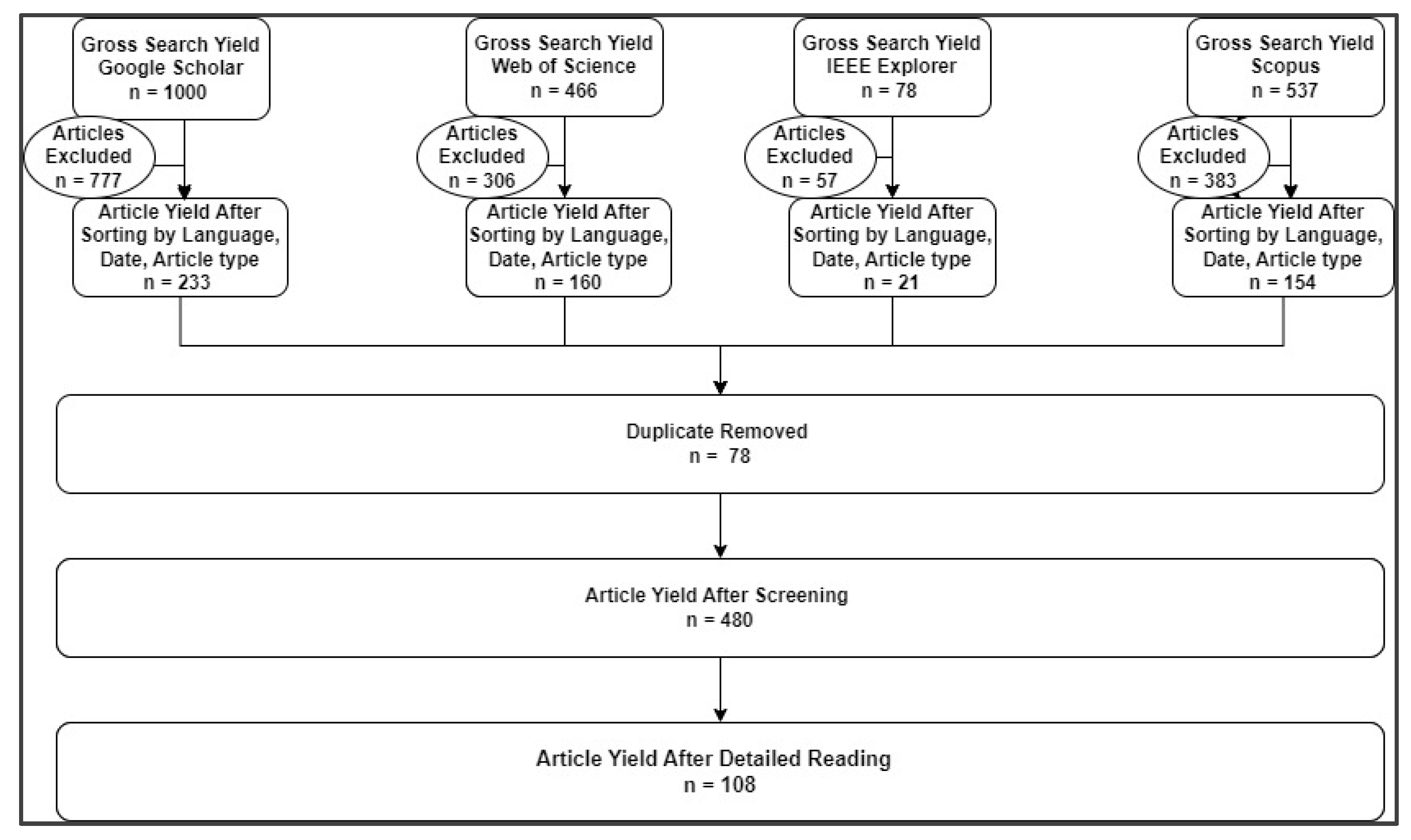
2. Materials and Methods

Electronic databases such as Scopus and Web of Science are essential sources of scientific publications for peer-reviewed journals suitable for systematic reviews. For this review, we utilised Web of Science, IEEE Explorer Scopus, and Google Scholar to search for relevant peer-reviewed publications. A broad mixture of systematically generated search words was used, including “remote sensing” and “grassland biomass”, to yield a widespread list of publications. A search with these keywords returned a number of peer-reviewed publications with 466 from Web of Science, 78 from IEEE Explorer, 537 from Scopus and 1000 from Google Scholar (Figure 1). We then applied a search filter to select the studies that achieved the following criteria: (1) attempted to develop remote sensing-based AGGB models; (2) were published in English from 1972 to 2020, following the launch of the first space-borne satellite; and (3) were peer-reviewed and published in scientific journals. Figure 1 portrays the PRISMA flow of the publication retrieval procedure. Based on the titles and abstracts, we performed a high-level screening of the articles to check if they met the stated filtering condition. We then downloaded the articles that met the filtering criteria, were available in a portable document format (pdf), were accessible in full length for further reading and analysis, and excluded those that were outside the scope of the above-mentioned filtering criteria. The publication that met the selection criteria summed to 108 and were subjected to data extraction and analysis. Table S1 (Supplementary Materials) provides a full list of the publications analysed in this review.
We used the built-in export function in the Web of Science, Scopus, IEEE Explorer, and Google Scholar databases to export the metadata of the searched publications to a Microsoft Excel spreadsheet (Microsoft Corporation, Redmond, WA, USA). Basic publication attributes such as the author, title, journal name, and year were extracted and exported. We then manually extracted additional publication attributes including the study site, geographic coordinates, sampling procedure, platform and sensor type, and spatial resolution, as well as predictor variables and methods through reading to expand and design a comprehensive database to achieve the intended goal of our review. As in Zolkos et al. [28], we also extracted the coefficient of determination statistic (R2) per data type, sensor as well as grassland types for the best remote sensing-based AGGB algorithm. For the purpose of this review, we only considered the coefficient of determination of the models developed using the training data.
To track the milestones of the remote sensing-based AGGB estimations, statistical frequencies were computed using MS Excel and SPSS. This assisted in observing and identifying trends in terms of the grassland type, geo-location and publications, platforms and sensors, predictor variables and algorithms, as well as the sampling procedure used in the literature. For the geographical trends, we imported the extracted geographical coordinates of where the studies were conducted into a Geographical Information System (GIS) software (Version 10.10) and created a proportional symbol map to visualise the frequency per country. As in Ma et al. [29], we also computed the mean measure and standard deviation of the coefficient of determination for sensor type and grassland type. We did this to compare the accuracies of the models across data types, sensor and grassland types using the coefficient of determination (R2) statistic as a measure. To do this, we grouped the multiple R statistics data per sensor and grassland types and plotted box plots. Furthermore, based on the range of spatial resolution found, we categorised the spatial resolution into six subcategories to be able to detect the trends in the use of spatial resolution in the images utilised. The studies reported a mix of findings and necessitated the need to omit some studies that did not report the required attributes. As a result, the number of collected statistics depends on whether the reviewed studies reported it or not. To identify the gaps and challenges, we manually extracted the text through reading, and grouped them into themes.

3. Results

3.1. Milestones of Remote Sensing-Based AGGB Retrieval

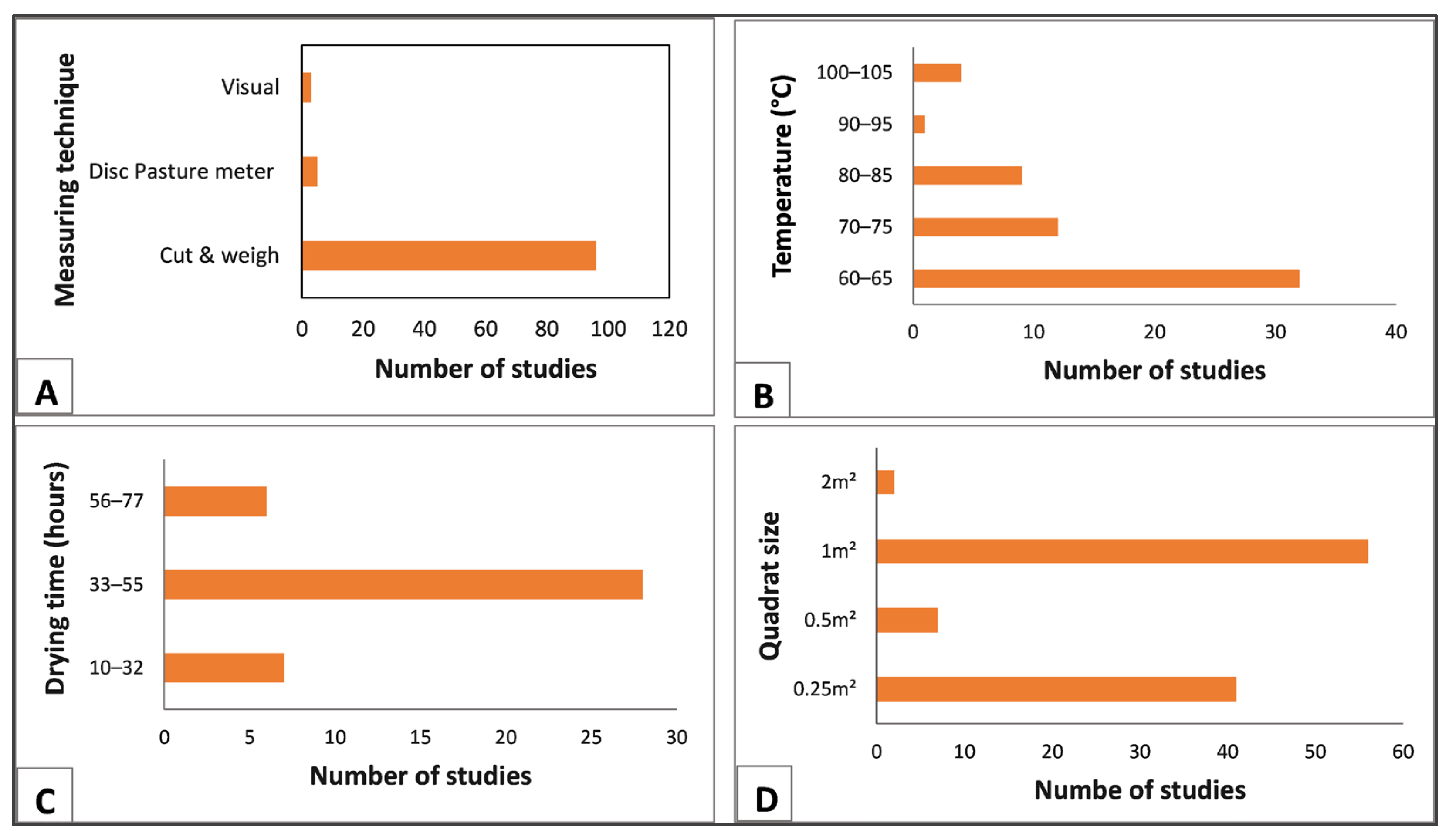
3.1.1. Sampling and Analysis Protocol for Training and Validation Purposes

Grasslands store carbon in the form of living and dead biomass [13]. Grass biomass is the organic material from both below and above the ground (either living or dead). Above-ground grass biomass encompasses all organic matter living above the ground [30]. While direct measurements of AGGB are obtainable through unfeasible and costly ground surveys, remotely sensed methods serve as an indirect means of retrieving AGGB [31]. With this approach, the grass biomass is indirectly inferred from satellite imagery where the relationships between satellite-derived indices and field biomass samples are established [14,32]. According to Chave et al. [31] “Remote sensing missions are dependent on accurate and representative in situ datasets for the training of their algorithms and product validation”.
Ali et al. [27] listed several methods used to collect AGGB samples for training and validating remote sensing data including visual, cut and dry, rising plate meter, and field spectroscopy. Within the reviewed literature, the harvesting (cut and dry) method remains the most heavily utilised destructive method to collect in situ AGGB samples for training and validating remote sensing algorithms (Figure 2A). A small number of studies utilised the rising plate meter, followed by the visual technique. For studies that adopted the clipping approach, the next step was to dry and weigh the clipped grass biomass samples in the laboratory at specific time frames and temperatures. As shown in Figure 2B, 65 degrees Celsius was the most frequently used temperature to dry the grass samples, followed by 80 and 70 °C. A few studies dried the grass biomass samples at 95 °C. Figure 2C shows that most studies dried the clipped grass samples over 48 h, followed by 72 and 24 h. Figure 2D shows the sizes of the subplots (n = 74) used when clipping the grass biomass samples. Of the 74 studies, 52% used 1 m2 subplots, followed by 0.25 m2.

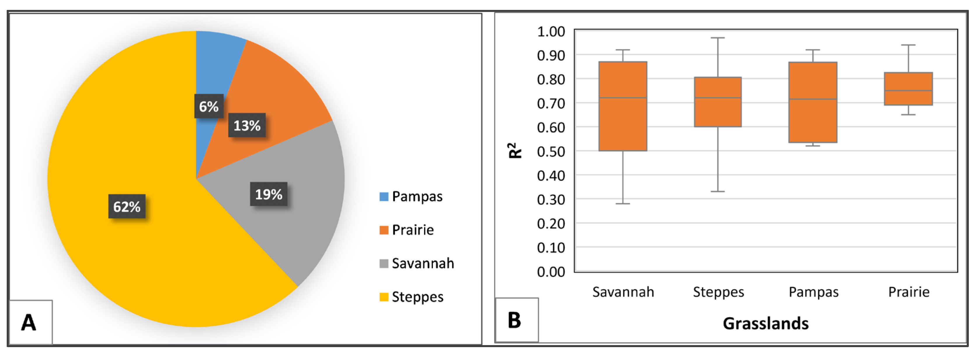
3.1.2. Grassland Types Covered in the Reviewed Studies

In order to identify the trends in grassland types, we grouped them based on their geographical location. The trends from the surveyed literature show that four types of grasslands were studied (Figure 3). Of the publications reviewed (n = 108), 62% of the remote sensing-based algorithms were developed and tested in the steppe grasslands, followed by the savannah grasslands (19%) and the prairie grasslands (13%), while the Pampas grasslands were rarely investigated (6%).
Figure 3B shows a box plot of the coefficient of determination of the remote sensing-based AGGB retrieval algorithm categorised by the grassland type. The grassland retrieval algorithms from the selected studies have medians that are in close range across the grassland type. Specifically, the savannah grasslands show more variability of R2 values (0.28–0.94), followed by the Pampas (0.33–0.97) and the steppe, while the prairie grasslands show the least variability. The prairie grasslands had a marginally higher mean (0.75) R2 compared to the savannah grasslands. The models developed in the savannah grasslands show high variability compared to the prairie grasslands.

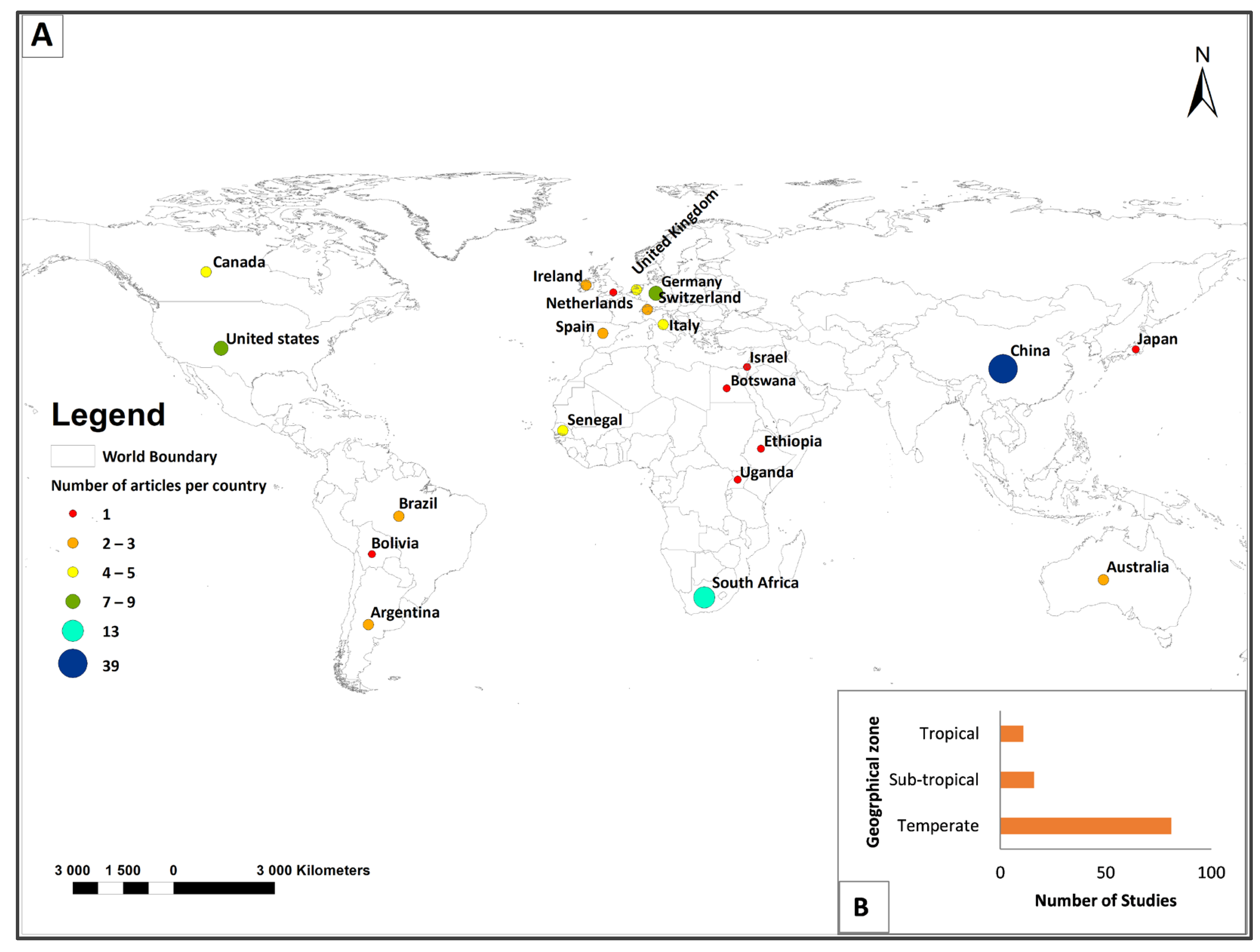
3.1.3. Geographical and Temporal Gradients Covered

The results from a geographical trend analysis show that remote sensing-based algorithms for estimating the AGGB were tested in 24 countries. However, an alarming gap was observed in terms of the regions studied (Figure 4A). Specifically, the top five countries in which the algorithms were tested the most were China, South Africa, Germany, the United States of America, and Italy. China yielded the highest proportion of studies (36%) that developed remote sensing-based algorithms for grass biomass retrieval. South Africa had the second largest number of studies (12%) while the USA and Germany contributed small percentages (8 and 6%, respectively). The remaining countries such as Australia, Ireland, and Japan contributed the least (1%).
There are four geographical climate zones worldwide, viz. the frigid, temperate, sub-tropical, and tropical zones [33]. The results from a further assessment of the geographical zones in which the studies were undertaken shows that the biomass retrieval algorithms were developed mostly in the temperate zone. Fewer studies (<20) were conducted in the tropical and subtropical zones while no studies were conducted in the frigid zone (Figure 4B).
Our findings show that Prince and Tucker made the first attempt to develop remote sensing-based algorithms to retrieve the AGGB in 1986. As shown in Figure 5, based on the surveyed literature, two studies on AGGB estimation were conducted between 1986 and 2005, followed by a gradual increase between 2006 and 2009. Subsequently, a decrease in the number of publications occurred between 2010 and 2013. The number of remote sensing-based AGGB studies gradually increased from 2014, with more than six publications per year. The largest number of studies were carried out in 2019 (13 studies).
We observed an inconsistent trend in the number of publications across the years of the survey. In particular, the years 1986–2005 accumulated the lowest yield in the number of publications, followed by a steady increase in the period 2006–2009. Another drop in the number of publications was observed in the period 2010–2013 and a gradual increase in the period 2014–2020.

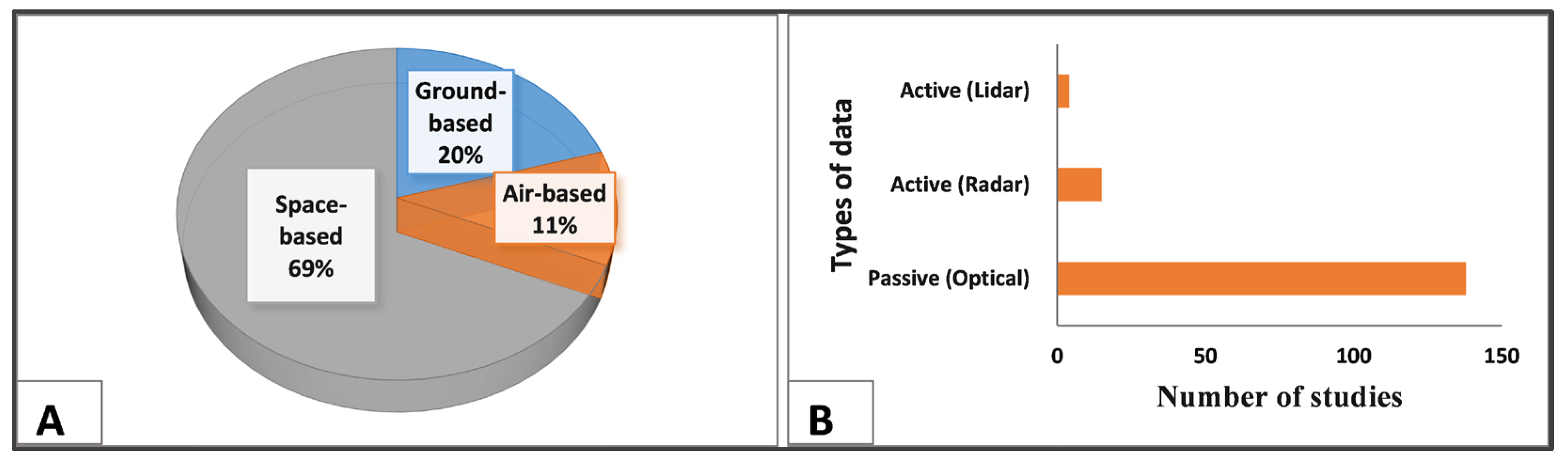
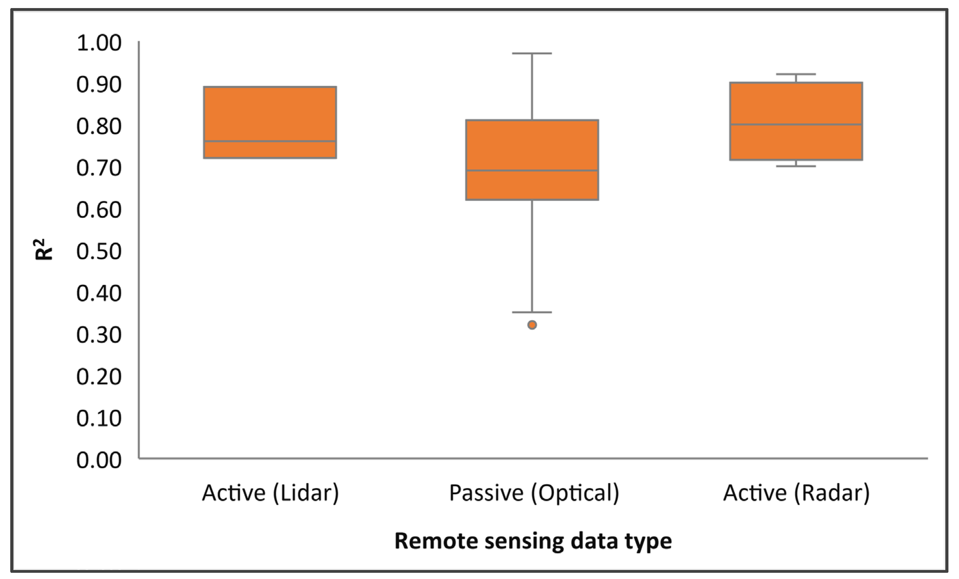
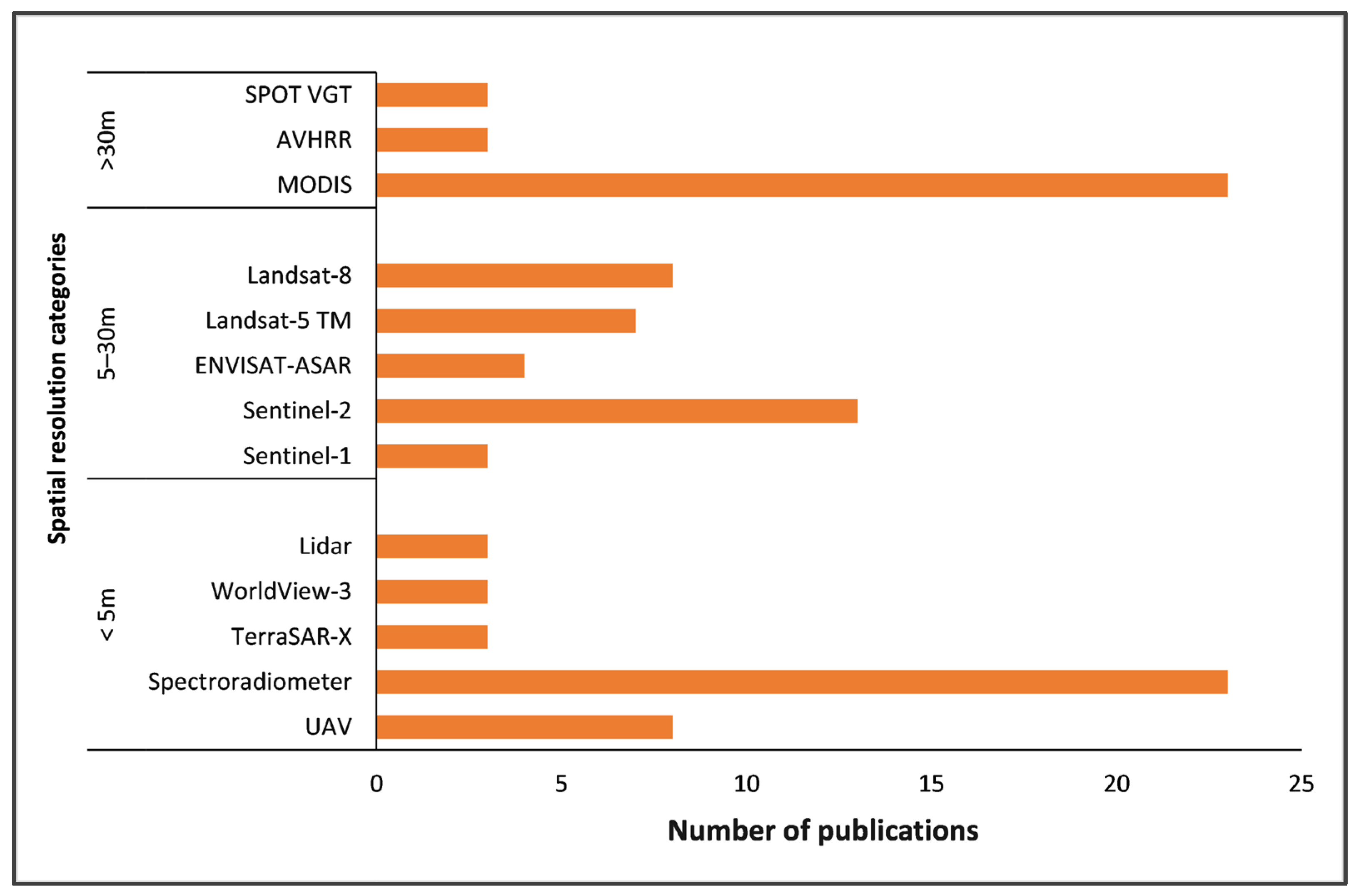
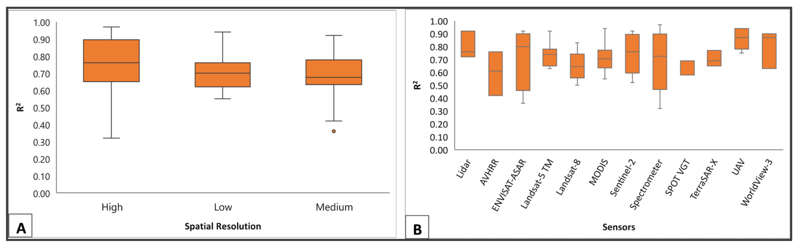
3.1.4. Platform and Sensor Configurations

The findings from the investigated literature (n = 108) show that a variety of platforms and sensors were used. From a platform perspective, the majority of the studies used sensors from space-borne platforms (69%), followed by sensors from ground-based platforms (20%), and lastly air-borne (11%) (Figure 6A). The images from optical sensors are the most heavily utilised amongst those selected for developing grass biomass retrieval models, followed by those from radar sensors. Light detecting and ranging (lidar) sensors were rarely utilised (Figure 6B).
We further assessed if the remote sensing data type utilised had an impact on the performance of the AGGB algorithm by plotting boxplots using the coefficient of determination (R2) as presented in Figure 7. The median overall coefficient of determination for all the remote sensing data types was above 0.6. Radar-based AGGB retrieval algorithms achieved the highest median R2 compared to optical data. As shown in Figure 7, the accuracies reported for the optical data in the surveyed literature show a large variability compared to the accuracies of radar. The graph also indicates that there are no significant differences between data types although there is much variability in the accuracies of the algorithm derived using passive data.
From an individual sensor perspective, Table 1 shows a variety of sensors that were applied in the AGGB estimation studies. Of the 33 types of sensors applied in the literature under investigation, 72% were optical, 22% were radar and 6% were lidar. The top four sensors that were employed the most were in the optical range and included MODIS, spectrometers, Landsat-8, and Sentinel-2. MODIS and spectroradiometers were the overall most frequently used sensors for AGGB estimation. Within the radar sensor range, ENVISAT ASAR was the most frequently used followed by Sentinel-1 (Table 1). Unlike optical sensors, radar sensors such as TerraSAR, CosmoSkyMed, AlosPal-SAR, and Quikscat were utilised in fewer studies. Table 2 shows the studies that applied radar in relation to the grassland type. The savannah grasslands were investigated in three of the studies listed in the table.
A further quantitative analysis of the spatial resolution of sensors used in the selected literature shows that the spatial resolution of the sensor utilised in the reviewed literature varied considerably. The majority of the studies employed sensors with spatial resolution >30 m and 5–30 m and lastly 0–5 m (Figure 8). The most widely used sensors were MODIS in the >30 m spatial resolution range and Spectroradiometer in the 0–5 m spatial resolution range.
We then assessed if the spatial resolution influenced the accuracies obtained in these studies. To do this, we grouped the sensors based on their spatial resolution and classified them as high (≤5 m), medium (6–30 m), and low (>30 m). As shown in Figure 9A, there is a relationship between the spatial resolution and the performance of the model. At a higher spatial resolution, the studies consulted achieved high accuracies, with a mean prediction accuracy of 0.75, while at a lower spatial resolution, low prediction accuracies were reported. In addition, at the medium spatial resolution, the studies obtained highly variable accuracies ranging from 0.28 to 0.75.
Figure 9B shows the median R2 per sensor. Unmanned aerial vehicle (UAV)-based sensors had the highest median coefficient of determination, followed by lidar and Sentinel-3. Generally, sensors with low spatial resolution seem to perform poorly, as also shown in this analysis. Furthermore, the findings from the literature revealed an insignificant variability across the estimates from each sensor class which had similar minimum RSE values.

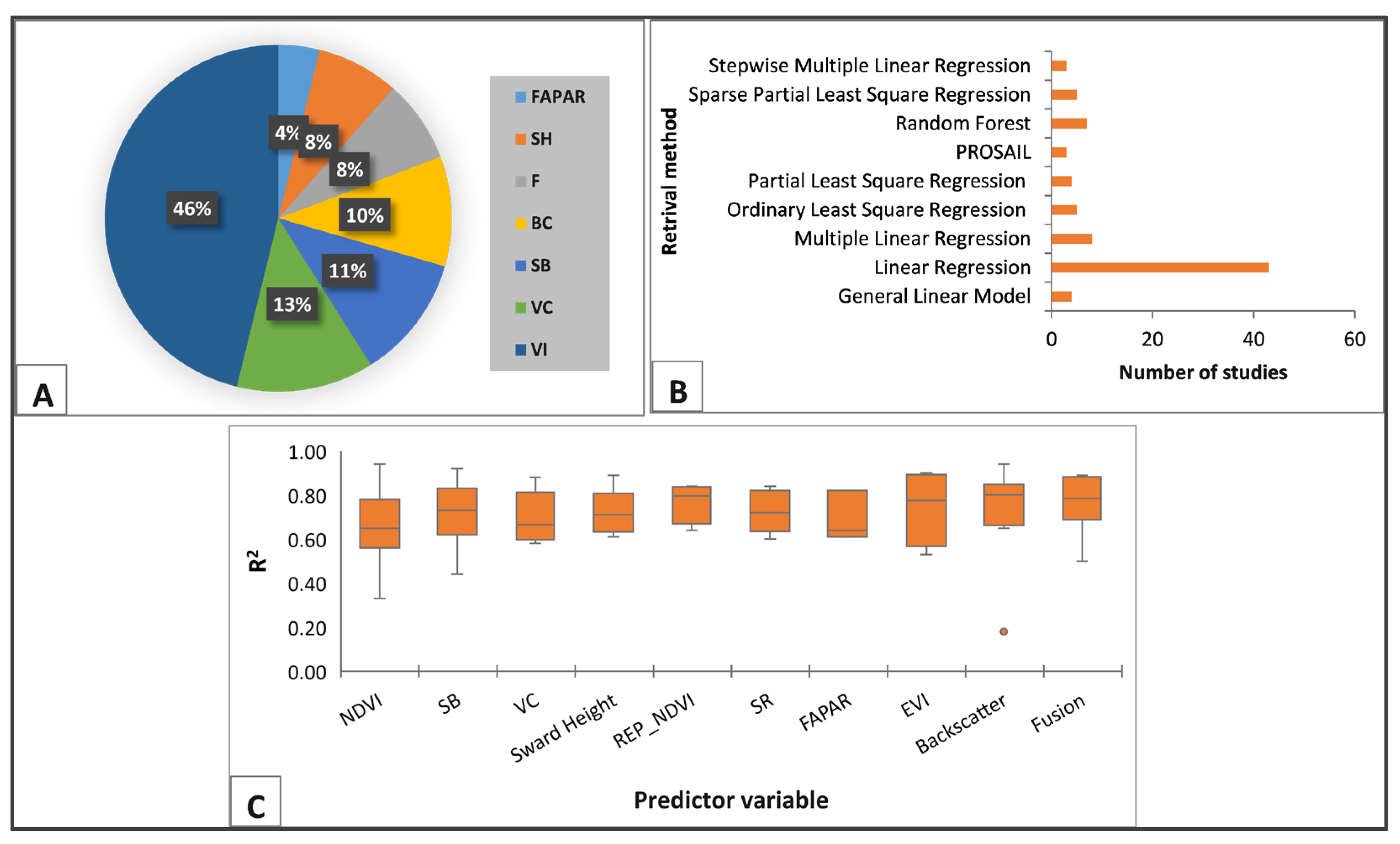
3.1.5. Predictor Variables Commonly Used in AGGB Studies

Several predictor variables (Table 3), such as raw spectral bands (SB), vegetation indices (VI), backscatter coefficients (BC), sward height (SH), fraction of photosynthetically active radiation (FAPAR), agrometeorological variables (rainfall and temperature), topographical variables and a combination of multiple variables (VC) have been widely utilised in remote sensing AGGB. Of the predictor variables (n = 78) (Figure 10A), 48% of the studies used vegetation indices as inputs in the developed models for estimating the AGGB, followed by a combination of two or more of the variables mentioned above (e.g., spectral bands + vegetation indices + climate variables). Furthermore, 12% of the studies used spectral bands while 11% of the studies used backscatter coefficients.
The results also revealed nine types of vegetation indices identified in the reviewed literature (Figure 10B). Of the vegetation indices, the Normalised Difference Vegetation Index (NDVI) was applied in half of the studies (n = 49), the red edge-based NDVI was the second largest, followed by the Enhanced Vegetation Index (EVI) (8%) and the Modified Soil-Adjusted Vegetation Index (MSAVI) (6%). Although the vegetation indices remain the most widely used input variables in remote sensing-based AGGB retrieval models, the accuracies obtained using these variables in the studies reviewed strongly vary compared to those obtained using backscatter coefficients, sward height and red edge-based NDVI variables (Figure 10C).

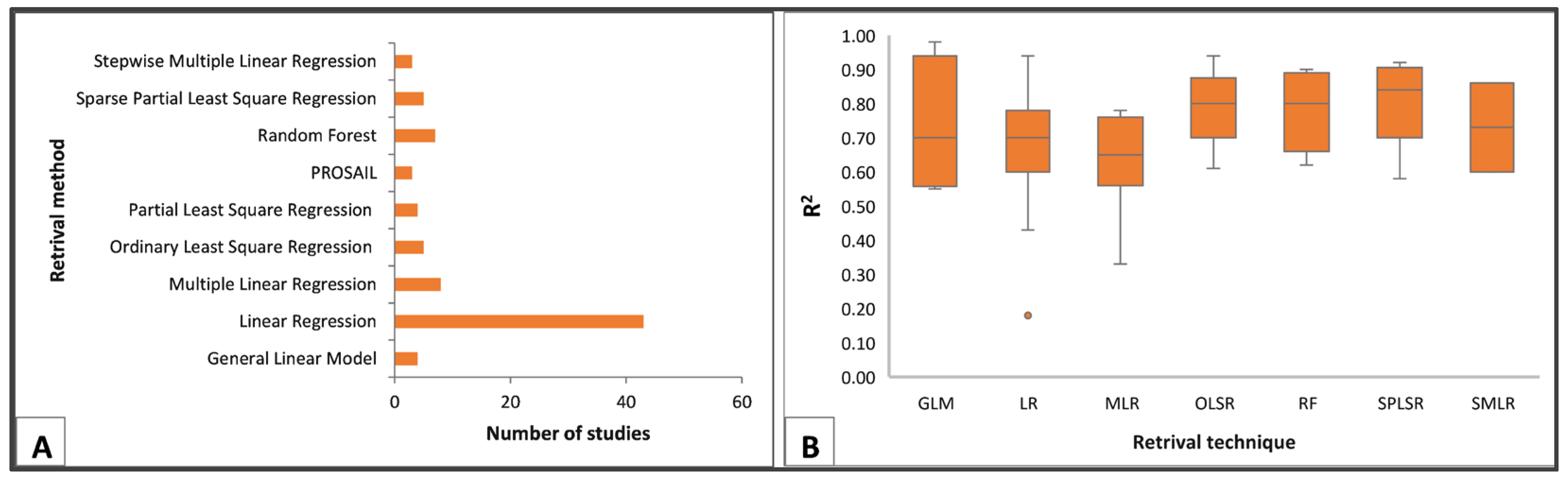
3.2. Algorithms Commonly Used in Remote Sensing-Based AGGB Studies

We detected nine regression (9) algorithms in the surveyed literature used to predict AGGB in 82 studies (Figure 11A). Fifty-two percent (52%) of the studies used linear regression methods. Only a few studies (8%) used machine learning algorithms such as Random Forest (RF) and 4% used a production efficiency model such as PROSAIL. These models yielded a median R2 value above 60% showing considerable prediction accuracies in estimating the AGGB (Figure 11B). SPLRS had the highest average prediction accuracy (85%) followed by RF andOLSR.

4. Discussion

4.1. Milestones of Remote Sensing-Based AGGB Retrieval

4.1.1. Sampling and Analysis Protocol for Training and Validation Purposes

The ability of remote sensing-based algorithms to accurately measure biomass varies with the type of grassland [52]. The evidence from the surveyed literature indicates that few studies developed remote sensing-based AGGB models in the savannah grasslands compared to the steppe grasslands. This could be because the steppe is the world’s biggest and most extensive grassland biome of the temperate climatic zone (i.e., the Eurasian Steppe) spreading from Hungary to China. However, the savannah ecosystem is characterised by a grass layer that co-exists with scattered trees and shrubs [53]. Surprisingly, savannahs and steppes seem to yield regression qualities that are in close range. The prairie and the Pampas grasslands showed similar trends, implying that the grassland type has little effect on the accuracies of estimates derived from remote sensing data. This is an intriguing observation given that the ecosystems are geographically located in different climate zones (temperate vs. subtropical). On the other hand, accuracies obtained from the Pampas grasslands seem less variable, suggesting some level of consistency across these studies. This could be attributed to the fact that the Pampas grasslands are less heterogeneous and consist of little to no trees [54] compared to savannahs, with a highly variable vegetation structure and species. The co-existence of grasses, trees, and shrubs in savannahs, specifically those on the African continent, present a different set of challenges for remote sensing approaches to retrieve AGGB, hence the inconsistent results detected in the reviewed literature. For example, savannahs in Sudan consist of scattered trees, which form a transition with the Sahara Desert vegetation whereas the savannahs found in Guinea consist of moist semi-deciduous woodlands which form a transition to the evergreen moist forests [53]. Furthermore, fire and herbivory activities pose a further challenge for the remote sensing-based AGGB estimation.

4.1.2. Geographical and Temporal Gradients Covered

A country-based analysis showed China as the highest contributor in terms of the output of AGGB estimation research. The dominance of China could be because it occupies a large portion of one of the most extensive Eurasian steppes in the world. Contrarily, developing countries contributed less, specifically those on the African continent. Compared to most developing countries, China strengthened its satellite surveillance capabilities for environmental monitoring with the launch of the HJ 1A/B optical imaging constellations in 2008 [55] as well as the HJ 1C radar satellite. Further improvements followed with the launch of the GaoFen-1 and 6 as well as Huanjing-2/A&B (HJ-2/A&B) [56]. Some countries in the global south also followed; for example, Egypt launched the Nilesat 101 in 1998 and South Africa launched the SumbadilaSat in 1999 which was only in orbit for 2 years [57]. Many developing nations find it difficult to maintain their own satellites due to the exorbitant expense of space rocket manufacturing and maintenance [57]. As a result, there is a lack of sufficient and sustainable access to satellite imagery for this region. Consequently, African countries still outsource remote sensing data from continents in the global north such as North America and Europe. Nevertheless, the dawn of open access policies to data and the Google Earth Engine (GEE) should stimulate the generation of new knowledge in these regions in the near future.
The findings also show a significant uneven trend in the annual production of AGGB retrieval studies across the years during the review period, particularly between the eras 1986–2005 and 2014–2020. The low research yields in the period 1986–2005 could be because fewer sensors (e.g., Landsat and MODIS) were operational. The steady increase in studies on AGGB after 2014 could be because of the gradual increase in sensor choice. For example, the Sentinel-2 constellation was launched in 2015 and made available at no cost. Nevertheless, an output of fewer than 20 articles per annum is inadequate to conclude on the optimal data, sensors, variables and algorithm for retrieving the AGGB in savannahs. Due to more available sensors (e.g., Landsat-9 and Sentinel-3), the rise is predicted to accelerate exponentially in the next few years. The improved capacity of computer hardware and software such as Google Earth Engine (GEE) that are designed to provide high-performing cloud-based computing, pre-processing algorithms as well as cloud-based storage should further increase the research outputs [22].

4.1.3. Platform and Sensor Configurations

The variability in remote sensing data types and sensors and their associated spatial resolution contributes to some level of uncertainty in the resulting AGGB estimates [58]. Optical sensors remain the most widely used, particularly from the MODIS and Landsat missions. MODIS and Landsat boast of long-term operations, and the free access policy associated with these constellations [59] further paved research methods to quantify the AGGB. The pool of studies utilising these sensors in comparison to others provides proof of this. The range of quality checked ready-to-use products [60] such as the MOD13Q1 from the MODIS constellation provide further benefits.
However, optical sensors such as MODIS have limitations [61,62,63], including their failure to collect data on days that are overcast, smoky, or misty [64]. The inability of optical sensors to capture data during these ad verse weather conditions impedes consistent monitoring, resulting in the omission of useful information for AGGB estimation. The selected studies show that optical sensors have a wide range of accuracies, implying inconsistent predictions.
In contrast, active sensors such as radar and lidar offer alternative datasets for estimating AGGB. These sensors boast about their ability to penetrate clouds and therefore provide data across all weather conditions. Despite this, radar was used in only 13 of the 108 studies reviewed. The low radar usage could be due to the cost tied to the data, therefore, limiting its widespread usage. Furthermore, radar-derived imagery is difficult to interpret for researchers with no prior knowledge and the processing is complex [65]. Nevertheless, studies reported improved accuracies in AGGB estimates from radar-based models, which were less variable, suggesting some level of consistency and dependable predictions. However, when considering the low-resolution sensors, it is evident that their accuracies might be comparatively lower. However, what is interesting is the remarkably narrower spread of values, excluding a notable outlier. This could indicate a higher level of consistency in accuracy across the low-resolution sensors. Contrarily, the high-resolution sensor shows a diverse range of accuracy values, which is further emphasized by the presence of an outlier. Thus, the concept that a higher resolution guarantees superior results is not a straightforward one. Nevertheless, the higher accuracies obtained for lidar and radar could have been influenced by the smaller number publications that were analysed in this review. The European Space Agency (ESA) currently distributes SAR data (i.e., Sentinel-1) at no cost, to help deal with the access issue. However, few of the reviewed studies tested Sentinel-1, signalling the need for further research.
For grass biomass studies, lidar metrics have also been used [66]. Unlike the popular optical data which views the two-dimensional (2D) attributes of grasses, lidar can detect three-dimensional (3D) attributes such as canopy height that can be used as proxies when quantifying the AGGB [67,68]. Despite this strength, few of the reviewed studies used lidar. This could be attributed to the fact that they cover small geographical footprints [69], which could be expensive to extend in the extensive tropical savannahs.
The review also identified the application of UAVs to a lesser extent in the surveyed studies. For example, only eight studies tested the utility of UAVs for deriving the AGGB. While higher accuracies were observed at the higher spatial resolution, the use of UAVs is limited to field scale [70] and their application in larger areas is restricted by their reliance on batteries. Furthermore, UAVs require several continuous flights for complete coverage in larger areas, which results in a large mosaic of tiles that need many hours to process [71].
While the use of a single sensor has individual shortfalls, combining sensors provides complimentary strength and fills in missing observations while ensuring data continuity [66]. For example, combining Sentinel-1, Landsat-8, and Sentinel-2 showed promising results, with Wang et al. [72] concluding that the estimation of the AGGB improved by more than 30% relative to the performance of Sentinel-1 alone at low vegetation cover and the optical data of Landsat-8 and Sentinel-2 at high vegetation cover. When combining spectroscopy and small-footprint waveform light detection and ranging (wLidar) data, Sarrazin et al. [67] concluded that fine-scale wLidar may not be able to provide accurate measurement of the herbaceous biomass and highlighted the need for further investigation during the peak growing season. However, in their review, Calleja et al. [71] found that the fusion of optical and UAV data was tested mostly in the ecology and precision agriculture. Few of the reviewed studies pursued fused optical and radar, lidar, UAV or vice versa, and as such, this remains an open field of research.
Few studies used several spatial resolutions associated with sensors to develop AGGB estimation models. Sensors with spatial resolution of 30 m and above were frequently used. This could be due to data accessibility and costs at specific spatial resolution intervals. Sensors with spatial resolution at 15 m and above (AVHRR, SPOT VEGT, MODIS, and Landsat) have been freely accessible for decades compared to their counterparts (Worldview-1/2, TerraSAR, lidar, or UAV-based sensors). Furthermore, earlier missions that piloted the use of remote sensing for monitoring vegetation attributes started with sensors at a spatial resolution of 15 m and above. For example, the Advanced Spaceborne Thermal Emission and Reflection Radiometer (ASTER) Mission at 15–30 m spatial resolution, the vegetation programme using SPOT VEGETATION at 1100 m, and the MODIS Land Group at 250, 500, and 1000 m spatial resolutions [58,72].
Sensors with spatial resolution ranging from 250 to >1000 m are suitable for studies at the national, continental, and global scale. Furthermore, sensors at 250 to >1000 m spatial resolution provide the balance between spatial resolution, surface area coverage and high frequency in data acquisition [13]. However, land surfaces are naturally heterogeneous and at this scale, the probability of detecting and capturing minute objects is quite low [12]. In addition, collecting ground-truthing samples at a 1000 m scale is not time- and cost-effective. This presents a large discrepancy between the size of the ground data and the spatial resolution of the image. Spectral mixture techniques were explored as an alternative to overcome the challenge of each pixel being a physical mixture of the multiple components weighted by the dominant area and the mixture spectrum is a linear combination of the end-member reflectance spectra [73]. On the bright side, the newly launched Sentinel-3 satellite presents a new dawn of opportunities in estimating and monitoring the AGGB at a larger scale. Compared to its predecessor (MERIS), Sentinel-3, specifically the Operational Land Imager (OLI), consists of six added spectral bands, a large swath width and offers improved signal-to-noise ratio (SNR) for monitoring vegetation condition [74]. Furthermore, while other constellations are freely available for academic and research purposes, but limited for commercial users, Sentinel-3 is anticipated to be freely available for both academic research and commercial uses.
Fewer studies explored sensors with spatial resolution ranging between 0 and 5 m and below. Although the spectral differences of grasslands can be captured accurately at a resolution ranging between 0 and 5 m, datasets at this scale are usually not readily accessible. The need for computers with large hard drives for storage further exacerbates the application limitation already associated with such datasets. Furthermore, 0–5 m pixel size is only applicable in localised areas of approximately 100 km2 and the processing time necessary to cover wider geographical areas is large [36].

4.1.4. Predictor Variables

The surveyed literature used several predictor variables as input into the AGGB estimation models. Broadband vegetation indices, particular NDVI, were the most widely used amongst the many variables. The frequent usage of NDVI could be because the index was pioneered specifically to monitor the vegetation conditions, and ultimately the AGGB. Nevertheless, NDVI is sensitive to the soil brightness and cloud shadow [75], rendering it unfit, especially in areas with low grass cover. To reduce the effects of the soil brightness, researchers pioneered the SR, EVI, and SAVI, although only a handful of studies have applied them for estimating the AGGB in the surveyed studies. Furthermore, NDVI is prone to saturation issues [16]. For example, in areas with high grass cover, NDVI tends to lose sensitivity and therefore produces inaccurate AGGB estimates. Narrowband widths (e.g., red edge position) from hyperspectral data are not prone to saturation issues [16]. Nevertheless, hyperspectral-derived predictor variables have “The curse of dimensionality” [76], a condition that occurs when analysing high-dimensional data that does not occur in low-dimensional spaces.
Other predictor variables including sward height [45], FAPAR [31,38], and backscatter coefficients [32], along with a combination of multiple variables (spectral bands + VI) [77] were developed. For example, FAPAR has been proven to improve prediction accuracies [61]. However, few of the studies reviewed applied these attributes.
From a performance perspective, NDVI is prone to obtaining low accuracies. Studies also show that the qualities of NDVI-based regressions as measured by the R2 vary widely, suggesting inconsistent and unreliable results. These findings are consistent with those of Zhao et al. [61] and could stem from the fact that most of the studies computed the NDVI from the broadband channels of optical sensors. According to Zhao et al. [78] “Broadband use the mean values of spectral information over broadband widths resulting in the loss of critical information that is available in specific narrow bands”. On the other hand, vegetation indices computed from narrow bands such as red edge-based NDVI show better performance. In particular, narrowband vegetation indices can maximise the contrast between grasslands and other land cover categories, therefore providing improved estimations.
The use of radar-derived metrics such as backscatter in savannah grasslands performed better in some studies [36,67]. For example, Wang et al. [36] demonstrated the capabilities of ENVISAT-ASAR and ALOS POLSAR to measure pasture biomass in Western Australia and obtained good results (i.e., R2 = 0.92). The low usage of radar-based metrics could be that in addition to the extreme cost, they require some sophisticated software and expert knowledge to interpret both the input and output results. Nevertheless, the launch of Sentinel-1 should extend the predictor variables outside the broadband optical channel to the microwave channels. Furthermore, while the highly priced hyperspectral-based narrow bandwidths provided improved AGGB estimates, Sentinel-2 MSI is also affordable and has robust spectral settings covering the red edge section of the electromagnetic spectrum. For example, Shoko et al. [77] demonstrated the abilities of the red edge-based NDVI derived from Sentinel-2 imagery.

4.1.5. Algorithms Developed

An analysis of the studies selected for the review showed that linear regression (LR) techniques were widely applied. This could be because linear equations are inherently simple and so are easy to operate and interpret [79]. The computation of linear equations is less time-efficient when compared to other retrieval algorithms. However, LR techniques are parametric and have normality assumptions, a condition that is not always representative of grass biomass on the ground.
Machine learning (ML) algorithms such as Random Forest have been developed and favoured for their non-reliance on assumptions. Furthermore, ML can handle a large number of datasets from heterogeneous landscapes, such as those in savannah ecosystems, which consist of trees, shrubs, and a layer of grasses, making them complex landscapes. However, in this review, fewer studies (8%) tested ML algorithms. Specifically, studies coupling ML algorithms with radar data to estimate the AGGB in savannah landscapes. Compared to conventional algorithms, ML algorithms are non-parametric and therefore independent of assumptions [80]. Nevertheless, the low usage of these algorithms could be because they are complex and not easily interpretable [81]. In fact, the majority of the ML algorithms have been categorised as a “black box”, meaning that they do not show the user the underlying process behind the prediction or provide features of importance [81].
To a smaller extent, Radiative Transfer models, specifically PROSAIL, have also been applied in the reviewed studies. PROSAIL is a physical-based model that depends on light absorption and scattering to compute vegetation properties. Compared to other statistical-based algorithms and ML models, radiation efficiency models are more robust and transferable as they use physical laws to express the transfer of light within grassland canopies. However, physical-based models lag since different combinations of plant traits can produce the same reflectance spectra. In parallel, physical models tend to perform better in retrieving some vegetation variables (e.g., chlorophyll content and leaf area index), but perform poorly with others (e.g., biomass). Furthermore, if one variable in the model is inaccurate, the whole model gets affected [24].
Today, although in its infancy, deep learning (DL) is emerging as the new generation of algorithms. DL algorithms have successfully delineated agricultural fields [82], classified satellite imagery [83] and mapped soil organic carbon [84]. In parallel, DL algorithms can handle “high dimensional data” and nonlinear relationships compared to their counterparts [70]. DL algorithms require intensive computation and programming skills to run them, hence their low application. However, there is a need for more experiments and observations, especially for regional and global biomass estimation studies, given the advent of “big data”.
From a performance perspective, the ML models yielded median R2 above 60%, showing considerable prediction accuracies across all the algorithms used in estimating the AGGB. Comparatively, linear regressions were observed to have a wide distribution of accuracies (40% to >80%) in the reviewed studies compared to ML algorithms, which seem to have a narrower distribution of R2 values. These results support those of Verrelst et al. [85] who found that the choice of a model for estimating biophysical parameters of grasses has an underlying impact on the accuracy of the results.

4.1.6. Sampling and Analysis Protocols

In situ data collection remains the most precise method of gathering representative biomass samples [13]. Remotely sensed AGGB estimates require a set of ground-truthing data to train and validate the models to be credible and reliable [14]. Scientists collect in situ grass biomass samples to ensure consistency between what they observe on the satellite image and the ground. Studies frequently harvest (cut and weigh) grass samples for testing and validating remote sensing-based AGGB estimates using 1 m2 quadrats. They then dry the collected samples mostly for 48 h at 65 degrees Celsius. However, the 1 m2 plot size does not match the spatial resolution of sensors mostly employed to extrapolate these plot-based measurements, producing some uncertainty in the resulting estimates [14]. Furthermore, [13] pointed that the time-to-time administration and execution of fieldwork activities is costly and tedious. He also observed that fieldwork costs are inversely proportional to the quantity and quality of the validation samples. In order to overcome the mismatch between the pixel size and in situ plot sizes and to compensate for the spatial resolution of the chosen sensors, studies often demarcate sampling plots equal to the spatial resolution of the sensor in less heterogeneous grasslands [17]. Nevertheless, UAVs are emerging as alternatives for validating remote sensing-based AGGB estimates [86]. Recently, portable spectrometers such as Field Spec 3 Max have also served as alternatives for ground-truthing of satellite images.

4.2. Research Challenges and Outlook

4.2.1. Research Challenges

The use of remote sensing to estimate the AGGB has shown considerable progress. However, from the reviewed studies, some degree of inconsistency in accuracy exists across the grassland types investigated, the predictor variables used, sensors, algorithms, as well as the sampling protocols adopted. Furthermore, researchers have encountered a myriad of obstacles in the pursuit of these estimates. From a grassland-type perspective, especially those consisting of sparse vegetation, the major concern was the influence of soil background [49], shadow from both clouds and topography, species diversity, and vegetation litter, which obscured the spectral response of the grasses [87]. In addition, grasslands in semi-arid areas such as the savannah consist of complex phenological stages, canopy structures, and species, compelling the need for sensors with a high temporal resolution. However, most readily available data covering the savannah have very low temporal resolutions. For example, MODIS offers coarse resolution (1000 m) at high temporal resolution (daily) for consistent monitoring purposes and is accessible freely, yet its application to localised studies is limited by its low spatial resolution. In areas with abundant rainfall, vegetation density increases at a faster rate, requiring more frequent observations [88].
As mentioned above, optical data remains the most widely used data type. However, clouds, topographic shadow, fire smoke, and haze, especially in the tropics and subtropics, with frequent cloud coverage, obscure the spectral response of the targeted vegetation using optical data. This constantly results in observation cut-offs, and consequently the loss of essential information. Radar sensors serve as alternative sources of datasets. Radar data has an important role in AGGB estimation, especially in areas such as the savannah ecosystem with its frequent cloudy conditions. While access to radar data is on the rise, some degree of limitation was reported in the literature, including its sensitivity to vegetation water content, soil moisture, winds, and humidity [89]. Furthermore, radar data analyses involved in pre-processing, removal of noise, and image processing require specialised software, knowledge, and skills to operate the software and ultimately interpret the results. Although radar datasets are available at no cost lately, there is still a relative lack of studies from which to draw concrete conclusions regarding their potential. The same observation can be made about lidar. However, lidar is expensive for applications in the savannah ecosystem.
Another pressing concern in the use of remote sensing to derive AGGB estimates is the issue of resolution (spatial, temporal, or spectral) [88]. Generally, landscapes across the globe are a collage consisting of a diverse range of vegetation classes configured differently (i.e., physiology and morphology), and savannah ecosystems are no exception. Sensors with a high spatial resolution were reported to address the issues around heterogeneity, which usually confuses pixels [13]. The major shortcoming associated with higher spatial resolution sensors is their price tag, but observations at lower spatial resolution risk the possibility of having more than one vegetation class in a single pixel [13]. The temporal resolution also presents further challenges. For example, monitoring vegetation variables frequently requires sensors with higher temporal resolutions. However, there is a lack of balance between the sensor’s spatial and temporal resolution. For example, an increase in the sensor’s pixel size implies a decrease in the temporal resolution [89]. In other words, gaining very precise estimates comes at the cost of omitting the time information associated with the observed vegetation variable [89]. Although high-resolution sensors have been proven to provide accurate estimates of the AGGB, they are, however, limited in scope because they do not capture images on a global scale, but rather at small footprints.
Several researchers reported saturation as an issue when retrieving the AGGB using remote sensing data [16]. For optical data, predictor variables such as the widely used NDVI tend to saturate at dense vegetation. A possible reason for this could be that when the density of vegetation reaches full coverage, the amount of red light that can be absorbed by leaves reaches a peak and, therefore, the sensitivity of reflectance starts diminishing with a rise in biomass [16]. The red edge position seems capable of overcoming the saturation encountered when using broadband-derived spectra and indices [16]. For radar data, saturation was obtained above 200 Mg ha−1 [89].
The most notable algorithm used in the consulted studies was statistical regression, specifically the linear function. However, statistical regression algorithms fail to detect the complex relationships that may be associated with the predicted variable without overfitting the models. Furthermore, these models seem to be limited to the specific sites in which they were developed, hence lacking both temporal and spatial transferability [14]. Researchers have attempted to transfer the models across sites with no luck in terms of accuracy, and encountering inconsistencies when transferring the models across temporal scales. Other studies highlighted the mismatch between the estimation and in situ measurement scale as a major concern [83]. For example, 1 m2 size subplots are normally used to collect samples for tuning the AGGB models and then scaled up to the selected sensor (e.g., 30 m) spatial resolution resulting in uncertain estimates [39].

4.2.2. Limitations of the Study

While a large number of studies pursuing optimal AGGB algorithms were conducted in the steppe ecosystems in the temperate climate zone, studies conducted in the tropical and subtropical grasslands, particularly the savannah ecosystem, are few, yet their different physiology and morphology may affect the models’ accuracies. Thus, the savannah ecosystem is open for further research. Furthermore, some publications were available in the abstract, while others were published in their native languages. We only considered publications that were published in English. In addition, we only considered articles that were available in PDF files. Furthermore, certain institutions subscribe to certain journals, resulting in limited access. All of this may have an impact on the number of publications as well as the geographical distribution of studies. Most remote sensing-based algorithms are subjected to a rigorous quality assessment to check for the fitness-for-purpose as well as the accuracy. While the latter is of great importance as it checks how close or far the predicted values are from the actual data modelled, the common model assessment index across all the studies was the R2. As such, for this review, we considered the commonly reported R2 index as a measure of the model performance.

4.2.3. Research Outlook

While considerable milestones have been realised in terms of the spatial distribution, sensors, development of predictor variables, and the engineering of extracting models, considerable research opportunities also exist. We provide the following summary:
  • Developed countries contributed more research on remote sensing-based AGGB compared to developing countries. As such, more research should be performed in the global south in order to promote an all-inclusive regional reporting.
  • Few studies applied remote sensors operating outside the optical channel of the electromagnetic spectrum (i.e., microwave) for retrieving the AGGB. Specifically, radar-derived metrics could add tangible value to the performance of biomass estimation models. The freely available Sentinel-1 offers an opportunity to quantify the AGGB in savannah ecosystems.
  • The integration of radar images shows promising results and a further exploration of the complimentary aspect of these sensors should improve the baseline models.
  • Although costly, lidar datasets seem promising in terms of accuracy and further studies should explore their full potential in AGGB estimation.
  • Despite their limitation, the vegetation indices remain the major predictor variables. Thus, improved accuracies of estimating the AGGB may be realised with the incorporation of supplementary variables such as sward height, FAPAR, agro-meteorological, and topographical variables.
  • From a radar perspective, the soil moisture and soil roughness should be taken into consideration during modelling since they contaminate the backscattering processes.
  • Many researchers have relied on the less transferable linear regression while machine learning approaches have not been fully explored. However, deep learning algorithms are emerging as the new dawn of algorithms and their utility in AGGB estimation is in its infancy, thereby leaving a gap for further research.
  • The mismatch between the estimating and validation scale reduces the accuracy of estimating the AGGB. The lack of consistency between the in situ measurement and sampling protocol further hinders the comparability across the studies. This signals the need to benchmark the sampling process.
  • It is also of interest to explore the use of the newly launched Sentinel-3 and Landsat-9 OLI in quantifying the AGGB in savannah ecosystems.
  • Future research on AGGB estimation should focus on the application of multi-source data and multi-temporal data available via cloud-based applications, including GEE, Microsoft Azure and Amazon Web Services (AWS).

5. Conclusions

This study synthesised findings of AGGB studies published in the literature to map the current state of the art and provide guidelines for model performance derived from decades of research. Authors have explored remote sensing-based models in steppes, while the African savannah ecosystems have not been fully explored. Savannahs consist of a grass layer that co-exists with scattered trees and shrubs, which may affect the results differently compared to the less heterogeneous steppe landscape. In optical remote sensing, particularly, MODIS and Landsat remain the main source of remotely sensed data for AGGB estimation even though they are affected by soil background and clouds, and are prone to saturation issues. Studies using SAR data, especially Sentinel-1, are scarce on a global scale, but the scarcity is more pronounced on the African continent despite being freely available. Vegetation indices, particularly NDVI, are a major AGGB predictor variable. However, the red edge position was pioneered to enhance the estimation of the AGGB and to reduce the saturation effects associated with broad bands. The existence of advanced machine learning algorithms dates back a while, yet researchers still rely on linear regression techniques. The newly developed deep learning algorithms should be explored further. Our results strongly suggest that the remote sensing-based AGGB findings are inconsistent across the consulted studies, making it difficult to draw conclusions on the optimal and universal model that can be used for estimating the AGGB in grasslands. There is, therefore, a need for standardising the remote sensing techniques, including the in situ data collection methods to ensure transferability of remote sensing-based AGGB models across multiple locations. Overall, this study has comprehensibly mapped the potential of remote sensing in retrieving AGGB estimates on a global scale.

Supplementary Materials

The following supporting information can be downloaded at: https://www.mdpi.com/article/10.3390/geomatics3040026/s1, Table S1: The 108 articles extracted from WoS, IEEE, Scopus and Google scholar.

Author Contributions

Conceptualization, R.M.; methodology, R.M.; investigation, R.M.; writing—original draft preparation, R.M.; writing—review and editing, R.M. and M.S.; supervision, G.C. and O.M.; funding acquisition, G.C. and O.M. All authors have read and agreed to the published version of the manuscript.

Funding

This research was funded by the Agricultural Research Council (ARC). The authors would like to thank the National Research Foundation (NRF) Research Chair in Land Use Planning and Management (Grant number: 84157) for funding parts of the fieldwork of this research.

Institutional Review Board Statement

Not applicable.

Informed Consent Statement

Not applicable.

Data Availability Statement

The secondary data used in this study is available in the following databases: WoS, IEEE Explorer, Scopus, and Google scholar.

Acknowledgments

The authors would like to thank the ARC’s Institute for Natural Resource and Engineering for providing the hardware and software used in this research. Thomas Fyfield is thanked for editing the manuscript. Furthermore, this forms part of the main author’s Ph.D. project.

Conflicts of Interest

The authors declare no conflict of interest.

References

  1. Scurlock, J.; Hall, D. The Global Carbon Sink: A Grassland Perspective. Glob. Chang. Biol. 1998, 4, 229–233. [Google Scholar] [CrossRef]
  2. Osborne, C.P.; Charles-Dominique, T.; Stevens, N.; Bond, W.J.; Midgley, G.; Lehmann, C.E. Human Impacts in African Savannas Are Mediated by Plant Functional Traits. New Phytol. 2018, 220, 10–24. [Google Scholar] [CrossRef] [PubMed]
  3. Ren, H.; Zhou, G. Estimating Senesced Biomass of Desert Steppe in Inner Mongolia Using Field Spectrometric Data. Agric. For. Meteorol. 2012, 161, 66–71. [Google Scholar] [CrossRef]
  4. Parr, C.L.; Lehmann, C.E.; Bond, W.J.; Hoffmann, W.A.; Andersen, A.N. Tropical Grassy Biomes: Misunderstood, Neglected, and Under Threat. Trends Ecol. Evol. 2014, 29, 205–213. [Google Scholar] [CrossRef]
  5. Ghosh, P.; Mahanta, S. Carbon Sequestration in Grassland Systems. Range Manag. Agrofor. 2014, 35, 173–181. [Google Scholar]
  6. Lan, X.; Tans, P.; Thoning, K.W. Trends in Globally-Averaged CO2 Determined from NOAA Global Monitoring Laboratory Measurements. Available online: https://gml.noaa.gov/ccgg/trends/gl_data.html (accessed on 7 August 2023).
  7. Chen, X.; Hutley, L.B.; Eamus, D. Carbon Balance of a Tropical Savanna of Northern Australia. Oecologia 2003, 137, 405–416. [Google Scholar] [CrossRef]
  8. Fiala, K. Belowground Plant Biomass of Grassland Ecosystems and Its Variation According to Ecological Factors. Ekológia 2010, 29, 182–206. [Google Scholar] [CrossRef]
  9. Adjorlolo, C.; Mutanga, O.; Cho, M.; Ismail, R. Challenges and Opportunities in the Use of Remote Sensing for C3 and C4 Grass Species Discrimination and Mapping. Afr. J. Range Forage Sci. 2012, 29, 47–61. [Google Scholar] [CrossRef]
  10. Sibanda, M.; Mutanga, O.; Rouget, M. Comparing the Spectral Settings of the New Generation Broad and Narrow Band Sensors in Estimating Biomass of Native Grasses Grown under Different Management Practices. GIScience Remote Sens. 2016, 53, 614–633. [Google Scholar] [CrossRef]
  11. Shoko, C.; Mutanga, O.; Dube, T. Progress in the Remote Sensing of C3 and C4 Grass Species Aboveground Biomass over Time and Space. ISPRS J. Photogramm. Remote Sens. 2016, 120, 13–24. [Google Scholar] [CrossRef]
  12. Meng, B.; Liang, T.; Yi, S.; Yin, J.; Cui, X.; Ge, J.; Hou, M.; Lv, Y.; Sun, Y. Modeling Alpine Grassland above Ground Biomass Based on Remote Sensing Data and Machine Learning Algorithm: A Case Study in East of the Tibetan Plateau, China. IEEE J. Sel. Top. Appl. Earth Obs. Remote Sens. 2020, 13, 2986–2995. [Google Scholar] [CrossRef]
  13. Lu, D. The Potential and Challenge of Remote Sensing-Based Biomass Estimation. Int. J. Remote Sens. 2006, 27, 1297–1328. [Google Scholar] [CrossRef]
  14. Eisfelder, C.; Kuenzer, C.; Dech, S. Derivation of Biomass Information for Semi-Arid Areas Using Remote-Sensing Data. Int. J. Remote Sens. 2012, 33, 2937–2984. [Google Scholar] [CrossRef]
  15. Svoray, T.; Shoshany, M. SAR-Based Estimation of Areal Aboveground Biomass (AAB) of Herbaceous Vegetation in the Semi-arid Zone: A Modification of the Water-Cloud Model. Int. J. Remote Sens. 2002, 23, 4089–4100. [Google Scholar] [CrossRef]
  16. Mutanga, O.; Skidmore, A.K. Narrow Band Vegetation Indices Overcome the Saturation Problem in Biomass Estimation. Int. J. Remote Sens. 2004, 25, 3999–4014. [Google Scholar] [CrossRef]
  17. Shoko, C.; Mutanga, O.; Dube, T. Determining Optimal New Generation Satellite Derived Metrics for Accurate C3 and C4 Grass Species Aboveground Biomass Estimation in South Africa. Remote Sens. 2018, 10, 564. [Google Scholar] [CrossRef]
  18. Debastiani, A.B.; Sanquetta, C.R.; Corte, A.P.D.; Rex, F.E.; Pinto, N.S. Evaluating SAR-Optical Sensor Fusion for Aboveground Biomass Estimation in a Brazilian Tropical Forest. Ann. For. Res. 2019, 62, 109–122. [Google Scholar] [CrossRef]
  19. Joshi, N.; Baumann, M.; Ehammer, A.; Fensholt, R.; Grogan, K.; Hostert, P.; Jepsen, M.; Kuemmerle, T.; Meyfroidt, P.; Mitchard, E.; et al. A Review of the Application of Optical and Radar Remote Sensing Data Fusion to Land Use Mapping and Monitoring. Remote Sens. 2016, 8, 70. [Google Scholar] [CrossRef]
  20. Ghasemi, N.; Sahebi, M.R.; Mohammadzadeh, A. A Review on Biomass Estimation Methods Using Synthetic Aperture Radar Data. Int. J. Geomat. Geosci. 2011, 1, 776. [Google Scholar]
  21. Sinha, S.; Jeganathan, C.; Sharma, L.K.; Nathawat, M.S. A Review of Radar Remote Sensing for Biomass Estimation. Int. J. Environ. Sci. Technol. 2015, 12, 1779–1792. [Google Scholar] [CrossRef]
  22. Kumar, L.; Mutanga, O. Remote Sensing of above-Ground Biomass. Remote Sens. 2017, 9, 935. [Google Scholar] [CrossRef]
  23. Kumar, L.; Sinha, P.; Taylor, S.; Alqurashi, A.F. Review of the Use of Remote Sensing for Biomass Estimation to Support Renewable Energy Generation. J. Appl. Remote Sens. 2015, 9, 097696. [Google Scholar] [CrossRef]
  24. Masenyama, A.; Mutanga, O.; Dube, T.; Bangira, T.; Sibanda, M.; Mabhaudhi, T. A Systematic Review on the Use of Remote Sensing Technologies in Quantifying Grasslands Ecosystem Services. GIScience Remote Sens. 2022, 59, 1000–1025. [Google Scholar] [CrossRef]
  25. Ali, I.; Greifeneder, F.; Stamenkovic, J.; Neumann, M.; Notarnicola, C. Review of Machine Learning Approaches for Biomass and Soil Moisture Retrievals from Remote Sensing Data. Remote Sens. 2015, 7, 16398–16421. [Google Scholar] [CrossRef]
  26. Mutanga, O.; Dube, T.; Ahmed, F. Progress in Remote Sensing: Vegetation Monitoring in South Africa. S. Afr. Geogr. J. 2016, 98, 461–471. [Google Scholar] [CrossRef]
  27. Ali, I.; Cawkwell, F.; Dwyer, E.; Green, S. Modeling Managed Grassland Biomass Estimation by Using Multitemporal Remote Sensing Data—A Machine Learning Approach. IEEE J. Sel. Top. Appl. Earth Obs. Remote Sens. 2016, 10, 3254–3264. [Google Scholar] [CrossRef]
  28. Zolkos, S.G.; Goetz, S.J.; Dubayah, R. A Meta-Analysis of Terrestrial Aboveground Biomass Estimation Using Lidar Remote Sensing. Remote Sens. Environ. 2013, 128, 289–298. [Google Scholar] [CrossRef]
  29. Ma, W.H.; Fang, J.Y.; Yang, Y.H.; Mohammat, A. Biomass Carbon Stocks and Their Changes in Northern China’s Grasslands during 1982–2006. Sci. China Life Sci. 2010, 53, 841–850. [Google Scholar] [CrossRef] [PubMed]
  30. FAO. Challenges and Opportunities for Carbon Sequestration in Grassland Systems; A Technical Report on Grassland Management and Climate Change Mitigation; Food and Agriculture Organization: Rome, Italy, 2010; pp. 1–57. [Google Scholar]
  31. Chave, J.; Davies, S.J.; Phillips, O.L.; Lewis, S.L.; Sist, P.; Schepaschenko, D.; Armston, J.; Baker, T.R.; Coomes, D.; Disney, M. Ground Data Are Essential for Biomass Remote Sensing Missions. Surv. Geophys. 2019, 40, 863–880. [Google Scholar] [CrossRef]
  32. Butterfield, H.; Malmström, C. The Effects of Phenology on Indirect Measures of Aboveground Biomass in Annual Grasses. Int. J. Remote Sens. 2009, 30, 3133–3146. [Google Scholar] [CrossRef]
  33. Mavridou, A.; Pappa, O.; Papatzitze, O.; Dioli, C.; Kefala, A.M.; Drossos, P.; Beloukas, A. Exotic Tourist Destinations and Transmission of Infections by Swimming Pools and Hot Springs—A Literature Review. Int. J. Environ. Res. Public Health 2018, 15, 2730. [Google Scholar] [CrossRef] [PubMed]
  34. Sang, H.; Zhang, J.; Lin, H.; Zhai, L. Multi-Polarization ASAR Backscattering from Herbaceous Wetlands in Poyang Lake Region, China. Remote Sens. 2014, 6, 4621–4646. [Google Scholar] [CrossRef]
  35. Moreau, S.; Le Toan, T. Biomass Quantification of Andean Wetland Forages Using ERS Satellite SAR Data for Optimizing Livestock Management. Remote Sens. Environ. 2003, 84, 477–492. [Google Scholar] [CrossRef]
  36. Wang, C.; Price, K.P.; Van Der Merwe, D.; An, N.; Wang, H. Modeling above-Ground Biomass in Tallgrass Prairie Using Ultra-high Spatial Resolution sUAS imagery. Photogramm. Eng. Remote Sens. 2014, 80, 1151–1159. [Google Scholar] [CrossRef]
  37. Hajj, M.E.; Baghdadi, N.; Belaud, G.; Zribi, M.; Cheviron, B.; Courault, D.; Hagolle, O.; Charron, F. Irrigated Grassland Monitoring Using a Time Series of terraSAR-X and COSMO-skyMed X-Band SAR Data. Remote Sens. 2014, 6, 10002–10032. [Google Scholar] [CrossRef]
  38. Schmidt, M.; Pringle, M.; Devadas, R.; Denham, R.; Tindall, D. A Framework for Large-Area Mapping of Past and Present Cropping Activity Using Seasonal Landsat Images and Time Series Metrics. Remote Sens. 2016, 8, 312. [Google Scholar] [CrossRef]
  39. Bao, N.; Li, W.; Gu, X.; Liu, Y. Biomass Estimation for Semiarid Vegetation and Mine Rehabilitation Using Worldview-3 and Sentinel-1 SAR Imagery. Remote Sens. 2019, 11, 2855. [Google Scholar] [CrossRef]
  40. Naidoo, L.; Van Deventer, H.; Ramoelo, A.; Mathieu, R.; Nondlazi, B.; Gangat, R. Estimating above Ground Biomass as an Indicator of Carbon Storage in Vegetated Wetlands of the Grassland Biome of South Africa. Int. J. Appl. Earth Obs. Geoinf. 2019, 78, 118–129. [Google Scholar] [CrossRef]
  41. Braun, A.; Wagner, J.; Hochschild, V. Above-Ground Biomass Estimates Based on Active and Passive Microwave Sensor Imagery in Low-Biomass Savanna Ecosystems. J. Appl. Remote Sens. 2018, 12, 046027. [Google Scholar] [CrossRef]
  42. Frolking, S.; Fahnestock, M.; Milliman, T.; McDonald, K.; Kimball, J. Interannual Variability in North American Grassland Biomass/Productivity Detected by SeaWinds Scatterometer Backscatter. Geophys. Res. Lett. 2005, 32. [Google Scholar] [CrossRef]
  43. Wang, J.; Xiao, X.; Bajgain, R.; Starks, P.; Steiner, J.; Doughty, R.B.; Chang, Q. Estimating Leaf Area Index and Aboveground Biomass of Grazing Pastures Using Sentinel-1, Sentinel-2 and Landsat Images. ISPRS J. Photogramm. Remote Sens. 2019, 154, 189–201. [Google Scholar] [CrossRef]
  44. Li, Z.; Guo, X. Can Polarimetric Radarsat-2 Images Provide a Solution to Quantify Non-Photosynthetic Vegetation Biomass in Semiarid Mixed Grassland? Can. J. Remote Sens. 2017, 43, 593–607. [Google Scholar] [CrossRef]
  45. Wijesingha, J.; Moeckel, T.; Hensgen, F.; Wachendorf, M. Evaluation of 3D Point Cloud-Based Models for the Prediction of Grassland Biomass. Int. J. Appl. Earth Obs. Geoinf. 2019, 78, 352–359. [Google Scholar] [CrossRef]
  46. Jiang, Y.; Tao, J.; Huang, Y.; Zhu, J.; Tian, L.; Zhang, Y. The Spatial Pattern of Grassland Aboveground Biomass on Xizang Plateau and Its Climatic Controls. J. Plant Ecol. 2015, 8, 30–40. [Google Scholar] [CrossRef]
  47. Ikeda, H.; Okamoto, K.; Fukuhara, M. Estimation of Aboveground Grassland Phytomass with a Growth Model Using Landsat TM and Climate Data. Int. J. Remote Sens. 1999, 20, 2283–2294. [Google Scholar] [CrossRef]
  48. Ullah, S.; Si, Y.; Schlerf, M.; Skidmore, A.K.; Shafique, M.; Iqbal, I.A. Estimation of Grassland Biomass and Nitrogen Using MERIS Data. Int. J. Appl. Earth Obs. Geoinf. 2012, 19, 196–204. [Google Scholar] [CrossRef]
  49. Ding, L.; Li, Z.; Wang, X.; Yan, R.; Shen, B.; Chen, B.; Xin, X. Estimating Grassland Carbon Stocks in Hulunber China, Using Landsat8 Oli Imagery and Regression Kriging. Sensors 2019, 19, 5374. [Google Scholar] [CrossRef] [PubMed]
  50. Li, Z.; Guo, X. Non-Photosynthetic Vegetation Biomass Estimation in Semiarid Canadian Mixed Grasslands Using Ground Hyperspectral Data, Landsat 8 OLI, and Sentinel-2 Images. Int. J. Remote Sens. 2018, 39, 6893–6913. [Google Scholar] [CrossRef]
  51. Ren, H.; Feng, G. Are Soil-Adjusted Vegetation Indices Better than Soil-Unadjusted Vegetation Indices for above-Ground Green Biomass Estimation in Arid and Semi-Arid Grasslands? Grass Forage Sci. 2015, 70, 611–619. [Google Scholar] [CrossRef]
  52. Su, J.; Bork, E. Influence of Vegetation, Slope, and Lidar Sampling Angle on DEM Accuracy. Photogramm. Eng. Remote Sens. 2006, 72, 1265–1274. [Google Scholar] [CrossRef]
  53. Mishra, N.B.; Young, K.R. Savannas and Grasslands. In Terrestrial Ecosystems and Biodiversity; CRC Press: Boca Raton, FL, USA, 2020; pp. 235–247. [Google Scholar]
  54. Ricard, M.F.; Berhongaray, G.; Viglizzo, E.F. The Argentine Pampas: A Novel Ecosystem at the Crossroad. Encycl. World’s Biomes 2020, 5, 117–127. [Google Scholar] [CrossRef]
  55. Xue, Y.; Li, Y.; Guang, J.; Zhang, X.; Guo, J. Small Satellite Remote Sensing and Applications–History, Current and Future. Int. J. Remote Sens. 2008, 29, 4339–4372. [Google Scholar] [CrossRef]
  56. Zhong, B.; Yang, A.; Liu, Q.; Wu, S.; Shan, X.; Mu, X.; Hu, L.; Wu, J. Analysis Ready Data of the Chinese GaoFen Satellite Data. Remote Sens. 2021, 13, 1709. [Google Scholar] [CrossRef]
  57. Oyewole, S. Space Research and Development in Africa. Astropolitics 2017, 15, 185–208. [Google Scholar] [CrossRef]
  58. Sánchez-Azofeifa, G.A.; Castro-Esau, K.L.; Kurz, W.A.; Joyce, A. Monitoring Carbon Stocks in the Tropics and the Remote Sensing Operational Limitations: From Local to Regional Projects. Ecol. Appl. 2009, 19, 480–494. [Google Scholar] [CrossRef] [PubMed]
  59. Zhu, Z.; Wulder, M.A.; Roy, D.P.; Woodcock, C.E.; Hansen, M.C.; Radeloff, V.C.; Healey, S.P.; Schaaf, C.; Hostert, P.; Strobl, P.; et al. Benefits of the Free and Open Landsat Data Policy. Remote Sens. Environ. 2019, 224, 382–385. [Google Scholar] [CrossRef]
  60. Wang, J.; Rich, P.M.; Price, K.P.; Dean Kettle, W. Relations between NDVI, Grassland Production, and Crop Yield in the Central Great Plains. Geocarto Int. 2005, 20, 5–11. [Google Scholar] [CrossRef]
  61. Zhao, F.; Xu, B.; Yang, X.; Jin, Y.; Li, J.; Xia, L.; Chen, S.; Ma, H. Remote Sensing Estimates of Grassland Aboveground Biomass Based on MODIS Net Primary Productivity (NPP): A Case Study in the Xilingol Grassland of Northern China. Remote Sens. 2014, 6, 5368–5386. [Google Scholar] [CrossRef]
  62. Liang, T.; Yang, S.; Feng, Q.; Liu, B.; Zhang, R.; Huang, X.; Xie, H. Multi-Factor Modeling of above-Ground Biomass in Alpine Grassland: A Case Study in the Three-River Headwaters Region, China. Remote Sens. Environ. 2016, 186, 164–172. [Google Scholar] [CrossRef]
  63. Zeng, N.; Ren, X.; He, H.; Zhang, L.; Zhao, D.; Ge, R.; Li, P.; Niu, Z. Estimating Grassland Aboveground Biomass on the Tibetan Plateau Using a Random Forest Algorithm. Ecol. Indic. 2019, 102, 479–487. [Google Scholar] [CrossRef]
  64. Prudente, V.H.R.; Martins, V.S.; Vieira, D.C.; e Silva, N.R.D.F.; Adami, M.; Sanches, I.D.A. Limitations of Cloud Cover for Optical Remote Sensing of Agricultural Areas across South America. Remote Sens. Appl. Soc. Environ. 2020, 20, 100414. [Google Scholar] [CrossRef]
  65. Tamiminia, H.; Salehi, B.; Mahdianpari, M.; Quackenbush, L.; Adeli, S.; Brisco, B. Google Earth Engine for Geo-Big Data Applications: A Meta-Analysis and Systematic Review. ISPRS J. Photogramm. Remote Sens. 2020, 164, 152–170. [Google Scholar] [CrossRef]
  66. Maesano, M.; Khoury, S.; Nakhle, F.; Firrincieli, A.; Gay, A.; Tauro, F.; Harfouche, A. UAV-Based LiDAR for High-Throughput Determination of Plant Height and above-Ground Biomass of the Bioenergy Grass Arundo donax. Remote Sens. 2020, 12, 3464. [Google Scholar] [CrossRef]
  67. Sarrazin, M.; Van Aardt, J.; Asner, G.; McGlinchy, J.; Messinger, D.; Wu, J. Fusing small-Footprint Waveform LiDAR and Hyperspectral Data for Canopy-Level Species Classification and Herbaceous Biomass Modeling in Savanna Ecosystems. Can. J. Remote Sens. 2011, 37, 653–665. [Google Scholar] [CrossRef]
  68. Wang, D.; Xin, X.; Shao, Q.; Brolly, M.; Zhu, Z.; Chen, J. Modeling Aboveground Biomass in Hulunber Grassland Ecosystem by Using Unmanned Aerial Vehicle Discrete Lidar. Sensors 2017, 17, 180. [Google Scholar] [CrossRef] [PubMed]
  69. Xu, Q.; Man, A.; Fredrickson, M.; Hou, Z.; Pitkänen, J.; Wing, B.; Ramirez, C.; Li, B.; Greenberg, J.A. Quantification of Uncertainty in Aboveground Biomass Estimates Derived from Small-Footprint Airborne LiDAR. Remote Sens. Environ. 2018, 216, 514–528. [Google Scholar] [CrossRef]
  70. Wang, Z.; Ma, Y.; Zhang, Y.; Shang, J. Review of Remote Sensing Applications in Grassland Monitoring. Remote Sens. 2022, 14, 2903. [Google Scholar] [CrossRef]
  71. Calleja, J.F.; Pagés, O.R.; Díaz-Álvarez, N.; Peón, J.; Gutiérrez, N.; Martín-Hernández, E.; Relea, A.C.; Melendi, D.R.; Álvarez, P.F. Detection of Buried Archaeological remains with the Combined Use of Satellite Multispectral Data and UAV Data. Int. J. Appl. Earth Obs. Geoinf. 2018, 73, 555–573. [Google Scholar] [CrossRef]
  72. Wang, G.; Liu, S.; Liu, T.; Fu, Z.; Yu, J.; Xue, B. Modelling above-Ground Biomass Based on Vegetation Indexes: A Modified Approach for Biomass Estimation in Semi-Arid Grasslands. Int. J. Remote Sens. 2019, 40, 3835–3854. [Google Scholar] [CrossRef]
  73. Tompkins, S.; Mustard, J.F.; Pieters, C.M.; Forsyth, D.W. Optimization of Endmembers for Spectral Mixture Analysis. Remote Sens. Environ. 1997, 59, 472–489. [Google Scholar] [CrossRef]
  74. Donlon, C.; Berruti, B.; Buongiorno, A.; Ferreira, M.-H.; Féménias, P.; Frerick, J.; Goryl, P.; Klein, U.; Laur, H.; Mavrocordatos, C. The Global Monitoring for Environment and Security (GMES) Sentinel-3 Mission. Remote Sens. Environ. 2012, 120, 37–57. [Google Scholar] [CrossRef]
  75. Bannari, A.; Morin, D.; Bonn, F.; Huete, A.R. A Review of Vegetation Indices. Remote Sens. Rev. 1995, 13, 95–120. [Google Scholar] [CrossRef]
  76. Timothy, D.; Onisimo, M.; Riyad, I. Quantifying Aboveground Biomass in African Environments: A Review of the Trade-Offs between Sensor Estimation Accuracy and Costs. Trop. Ecol. 2016, 57, 393–405. [Google Scholar]
  77. Shoko, C.; Mutanga, O.; Dube, T.; Slotow, R. Characterizing the Spatio-Temporal Variations of C3 and C4 Dominated Grasslands Aboveground Biomass in the Drakensberg, South Africa. Int. J. Appl. Earth Obs. Geoinf. 2018, 68, 51–60. [Google Scholar] [CrossRef]
  78. Zhao, D.; Huang, L.; Li, J.; Qi, J. A Comparative Analysis of Broadband and Narrowband Derived Vegetation Indices in Predicting Lai and Ccd of a Cotton Canopy. ISPRS J. Photogramm. Remote Sens. 2007, 62, 25–33. [Google Scholar] [CrossRef]
  79. Keith, A.; Marill, M.D. Advanced Statistics: Linear Regression, Part I: Simple Linear Regression. Acad. Emerg. Med. 2004, 11, 87–93. [Google Scholar]
  80. Barrett, B.; Nitze, I.; Green, S. Assessment of Multi-Temporal, Multi-Sensor Radar and Ancillary Spatial Data for Grasslands Monitoring in Ireland Using Machine Learning Approaches. Remote Sens. Environ. 2014, 152, 109–124. [Google Scholar] [CrossRef]
  81. Wadoux, A.; Minasny, B.; McBratney, A.B. Machine Learning for Digital Soil Mapping: Applications, Challenges and Suggested Solutions. Earth Sci. Rev. 2020, 210, 103359. [Google Scholar] [CrossRef]
  82. Sharifi, A.; Mahdipour, H.; Moradi, E.; Tariq, A. Agricultural Field Extraction with Deep Learning Algorithm and Satellite Imagery. J. Indian Soc. Remote Sens. 2022, 50, 417–423. [Google Scholar] [CrossRef]
  83. Pritt, M.; Chern, G. Satellite Image Classification with Deep Learning. In Proceedings of the 2017 IEEE Applied Imagery Pattern Recognition Workshop (AIPR), Washington, DC, USA, 10–12 October 2017. [Google Scholar] [CrossRef]
  84. Odebiri, O.; Odindi, J.; Mutanga, O. Basic and Deep Learning Models in Remote Sensing of Soil Organic Carbon Estimation: A Brief Review. Int. J. Appl. Earth Obs. Geoinf. 2021, 102, 102389. [Google Scholar] [CrossRef]
  85. Verrelst, J.; Malenovský, Z.; Van der Tol, C.; Camps-Valls, G.; Gastellu-Etchegorry, J.P.; Lewis, P.; North, P.; Moreno, J. Quantifying Vegetation Biophysical Variables from Imaging Spectroscopy Data: A Review on Retrieval Methods. Surv. Geophys. 2019, 40, 589–629. [Google Scholar] [CrossRef]
  86. Urbazaev, M.; Thiel, C.; Cremer, F.; Dubayah, R.; Migliavacca, M.; Reichstein, M.; Schmullius, C. Estimation of Forest Aboveground Biomass and Uncertainties by Integration of Field Measurements, Airborne LiDAR, and SAR and Optical Satellite Data in Mexico. Carbon Balance Manag. 2018, 13, 5. [Google Scholar] [CrossRef] [PubMed]
  87. Svoray, T.; Shoshany, M.; Curran, P.J.; Foody, G.M.; Perevolotsky, A. Relationship between Green Leaf Biomass Volumetric Density and ERS-2 SAR Backscatter of Four Vegetation Formations in the Semi-Arid Zone of Israel. Int. J. Remote Sens. 2001, 22, 1601–1607. [Google Scholar] [CrossRef]
  88. Li, M.; Zang, S.; Zhang, B.; Li, S.; Wu, C. A Review of Remote Sensing Image Classification Techniques: The Role of Spatio-Contextual Information. Eur. J. Remote Sens. 2014, 47, 389–411. [Google Scholar] [CrossRef]
  89. Hamdan, O.; Hasmadi, I.M.; Aziz, H.K.; Norizah, K.; Zulhaidi, M.H. L-Band Saturation Level for Aboveground Biomass of Dipterocarp Forests in Peninsular Malaysia. J. Trop. For. Sci. 2015, 27, 388–399. [Google Scholar]
Figure 1. The PRISMA workflow of literature search and selection used for the review.
Geomatics 03 00026 g001
Figure 2. A depiction of (A) field AGGB sample collection techniques; (B) drying temperature expressed in degrees Celsius adopted in the studies; (C) drying time expressed in hours; and (D) the subplot size utilised in the literature.
Geomatics 03 00026 g002
Figure 3. A depiction of (A) grassland types investigated in the reviewed studies, and (B) box plots showing median R2 for the distribution of grassland type investigated in the selected literature.
Geomatics 03 00026 g003
Figure 4. A depiction of (A) the geographical distribution of extracted literature by country, and (B) the geographical climate zones observed in the selected literature.
Geomatics 03 00026 g004
Figure 5. A depiction of the number of publications on remote sensing-based AGGB retrieval by year.
Geomatics 03 00026 g005
Figure 6. A depiction of (A) remote sensing platform, and (B) type of data used in the selected literature for AGGB retrieval.
Geomatics 03 00026 g006
Figure 7. Box plots showing median R2 by remote sensing data type. The dot shows outlier R2 values.
Geomatics 03 00026 g007
Figure 8. Spatial resolution range associated with the sensors utilised in the reviewed literature. Sensors that were utilised in less than three studies were excluded.
Geomatics 03 00026 g008
Figure 9. A depiction of (A) box plots showing R2 values for the categories of sensor spatial resolution utilised in the surveyed literature (high ≤ 5 m, medium = 6–30 m and low ≥ 30 m), and (B) box plots showing R2 values for the sensors utilised in the studies. Sensors utilised in less than three studies are excluded. Studies that did not report the R2 value were also excluded from this analysis. The dot shows outlier R2 values.
Geomatics 03 00026 g009
Figure 10. A depiction of (A) predictor variable commonly used for estimating AGGB (SB = spectral bands, VI = vegetation indices, BC = backscatter coefficients, SH = sward height, FAPAR = fraction of photosynthetically active radiation, VC = variable composite, F = fusion); (B) vegetation indices commonly used for estimating AGGB; and (C) box plots showing the R2 values per predictor variable utilised. Variables utilised in less than three studies are excluded. The dot shows outlier R2 values.
Geomatics 03 00026 g010
Figure 11. A depiction of (A) models commonly used to retrieve AGGB within the reviewed studies, and (B) box plots portraying the R2 values per model used in the surveyed studies (GLM = General Linear Model, LR = Linear regression, MLR = Multiple linear regression, OLSR = Ordinary least square regression, RF = Random Forest, SPLSR = Sparse Partial Least Square Regression, SMLR = stepwise multiple linear regression). Models utilised in less than three studies are excluded. The dot shows outlier R2 values.
Geomatics 03 00026 g011
Table 1. Number of publications per individual sensor.
SensorNumber of Studies
MODIS23
Spectroradiometer23
Landsat 818
Sentinel-213
AVHRR4
Landsat-54
Landsat-7 ETM+4
SPOT-54
SPOT VGT4
WorldView-24
ENVISAT ASAR4
UAV4
WorldView-33
PROBA-V3
Lidar3
Sentinel-13
TerraSAR-X2
European Remote-Sensing (ERS-1)2
ALOS PALSAR2
HJ1B-CCD22
RADARSAT2
COSMO-SkyMed (CSK)1
Hyperion1
Indian Remote Sensing1
MERIS1
HyMap1
Apex1
SSMI1
Ultrasonic distance sensor1
QuikScat1
SPOT-41
Digital camera1
SEA WIND1
Studies that applied more than one sensor were counted several times, SSMI = Special Sensor Microwave Imager.
Table 2. An overview of the studies that used radar sensors to estimate AGGB.
AuthorsSensorsCountryGrassland Type
Sang et al. [34]ENVISAT-ASARChinaSteppe
Moreau and Le Toan [35]ERS-1BoliviaSavannah
Wang et al. [36]ENVISAT-ASAR and ALOS POLSARAustraliaPampas
Svoray and Shoshany [15]ERS-1IsraelSteppe
Hajj et al. [37]TERRASAR-X-and COSMO SKYMEDFranceSteppe
Schmidt et al. [38]TERRASAR-X-AustraliaSavannah
[26]TERRASAR-XIrelandSteppe
Bao et al. [39]Sentinel-1ChinaPampas
Naidoo et al. [40]Sentinel-1South AfricaSavannah
Braun et al. [41]ENVISAT-ASAR, ALOS POLSAR and SSMISenegalSavannah
Frolking et al. [42]SEA WINDUnited StatesPrairie
Wang et al. [43]Sentinel-1United StatesPrairie
Li and Guo, 2017 [44]RADARSATCanadaPrairie
Table 3. A summary of the predictor variables that used in the surveyed literature.
Variable NameExpression/Spectral BandsExample Study
BackscatterHHAli et al. [27]
Canopy Sward HeightN/AWijesingha et al. [45]
Enhanced Vegetation Index (EVI)(R851 − R655)/(R851 + 6R655 − 7.8R482 + 1)Meng et al. [12]
Fraction of Photosynthetically Active Radiation (FAPAR)FAPAR = 1 − t − r + trsSchmidt et al. [38]
Modified Soil-Adjusted Vegetation Index (MSAVI)[2NIR + 1 − ((2NIR + 1)2 − 8(NIR − R)) 0.5]/2Jiang et al. [46]
Normalised Difference Vegetation Index (NDVI)NDVI = − (infrared band − red band)/(infrared band + red band)Ikeda et al. [47]
Normalised Band Depth Index (NBDI)NBDI = BD − Dc/BD + DUllah et al. [48]
Ratio Vegetation Index (RVI)RVI = NIR/RedDing et al. [49]
Red Edge-Based NDVI(R750 − R705)/(R750 + R705)Li and Guo [50]
Red Edge-Based Simple Ratio(R708 − R755)/(R708 + R755)Mutanga and Skidmore [16]
Simple Ratio (SR)SR = NIR/RedRen and Feng [51]
Soil-Adjusted Vegetation Index (SAVI)1 + L × (RNIR − RRED)/(RNIR + RRED) + LRen and Feng [51]
RNIR is the reflectance in the Near Infrared band, RRed is the reflectance in the Red band.
Disclaimer/Publisher’s Note: The statements, opinions and data contained in all publications are solely those of the individual author(s) and contributor(s) and not of MDPI and/or the editor(s). MDPI and/or the editor(s) disclaim responsibility for any injury to people or property resulting from any ideas, methods, instructions or products referred to in the content.

