


Relationships between Soil Moisture and Visible–NIR Soil Reflectance: A Review Presenting New Analyses and Data to Fill the Gaps

Abstract
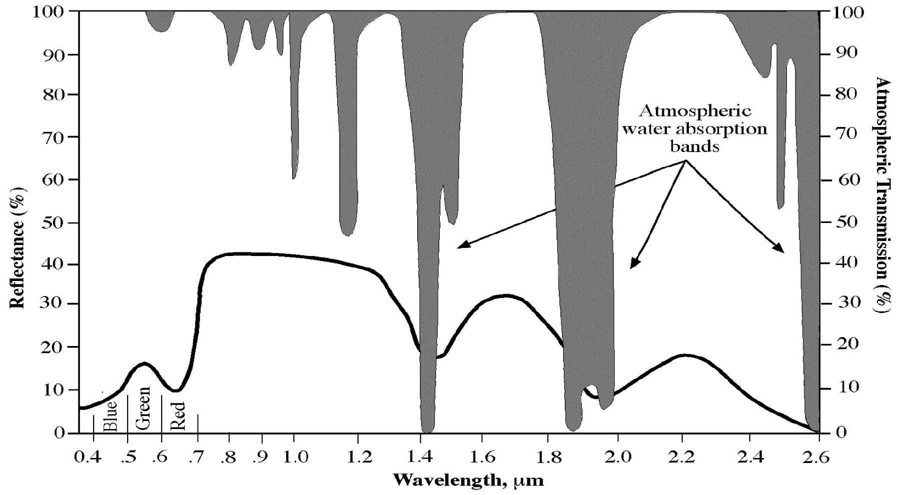
:1. Introduction
- 4.
- 5.
- 6.
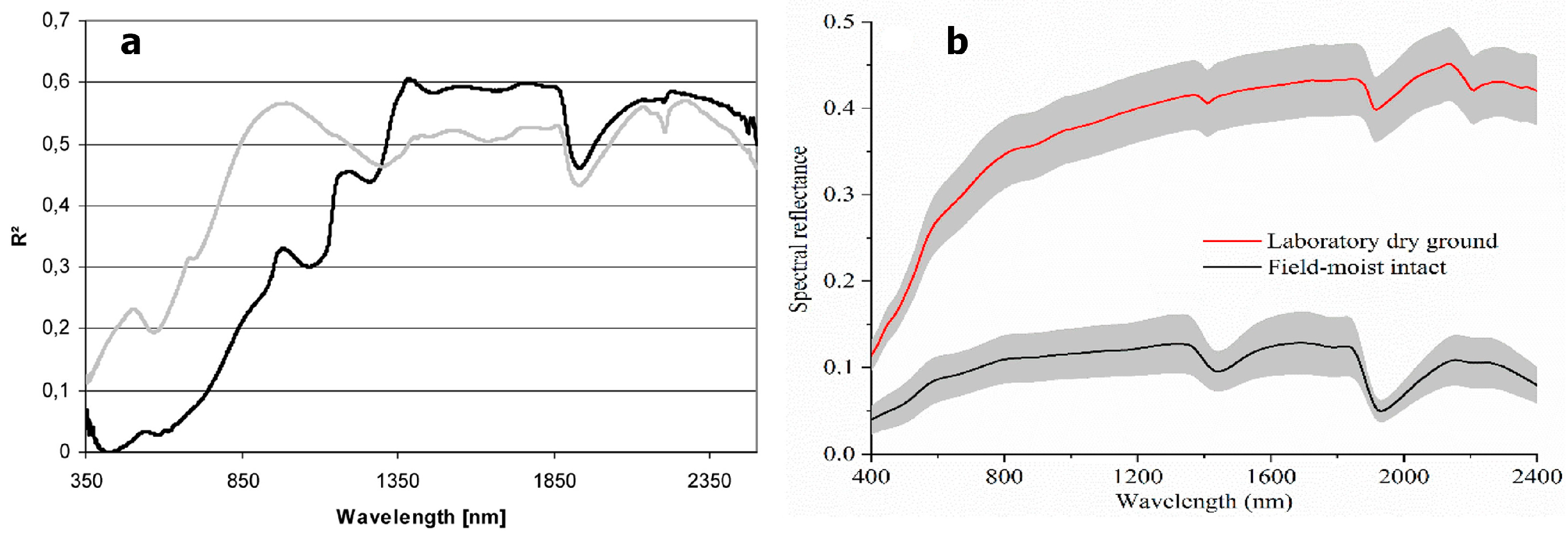
2. The Effects of Soil MC on Soil Reflectance—Insights from the Literature


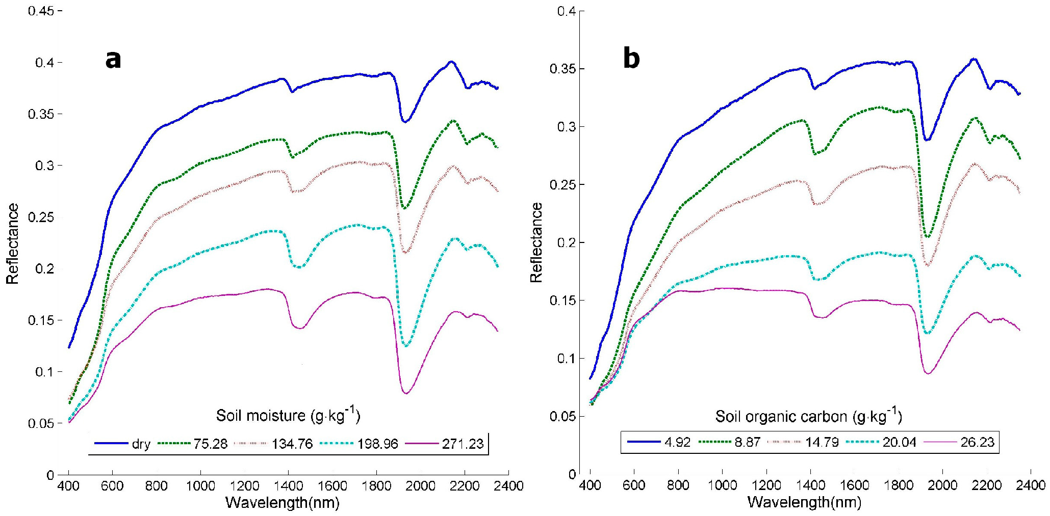
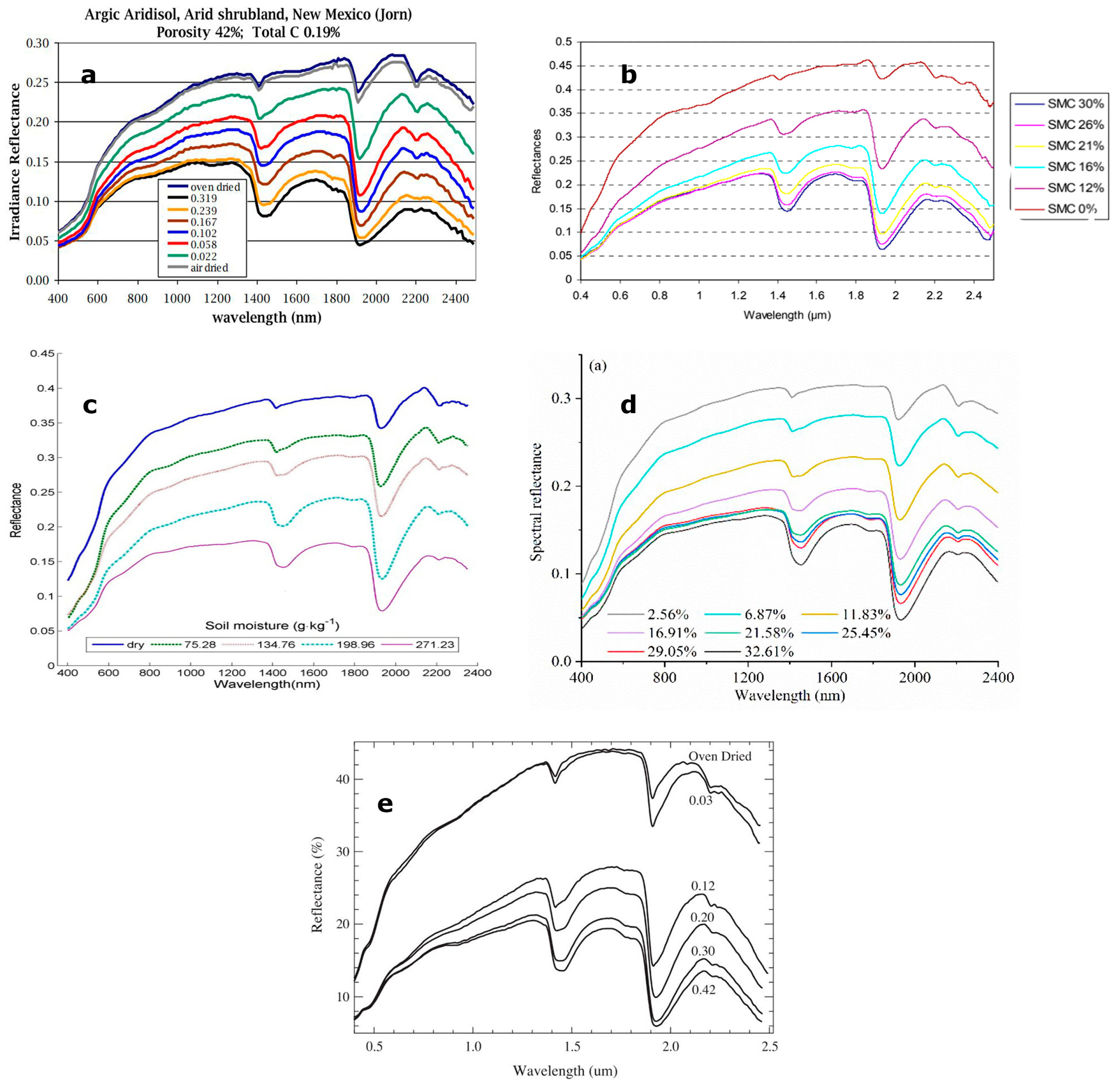
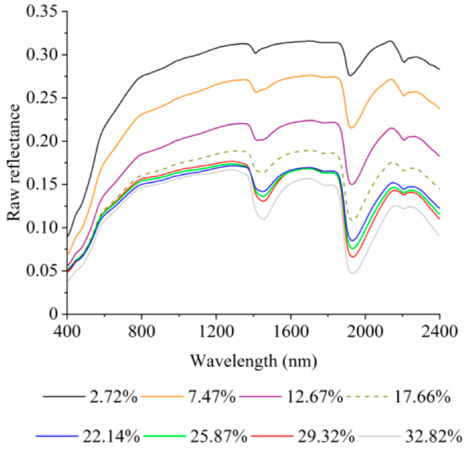
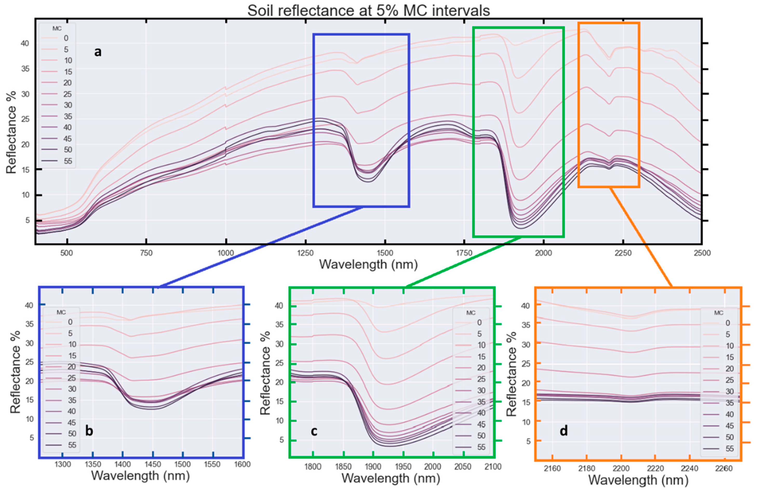
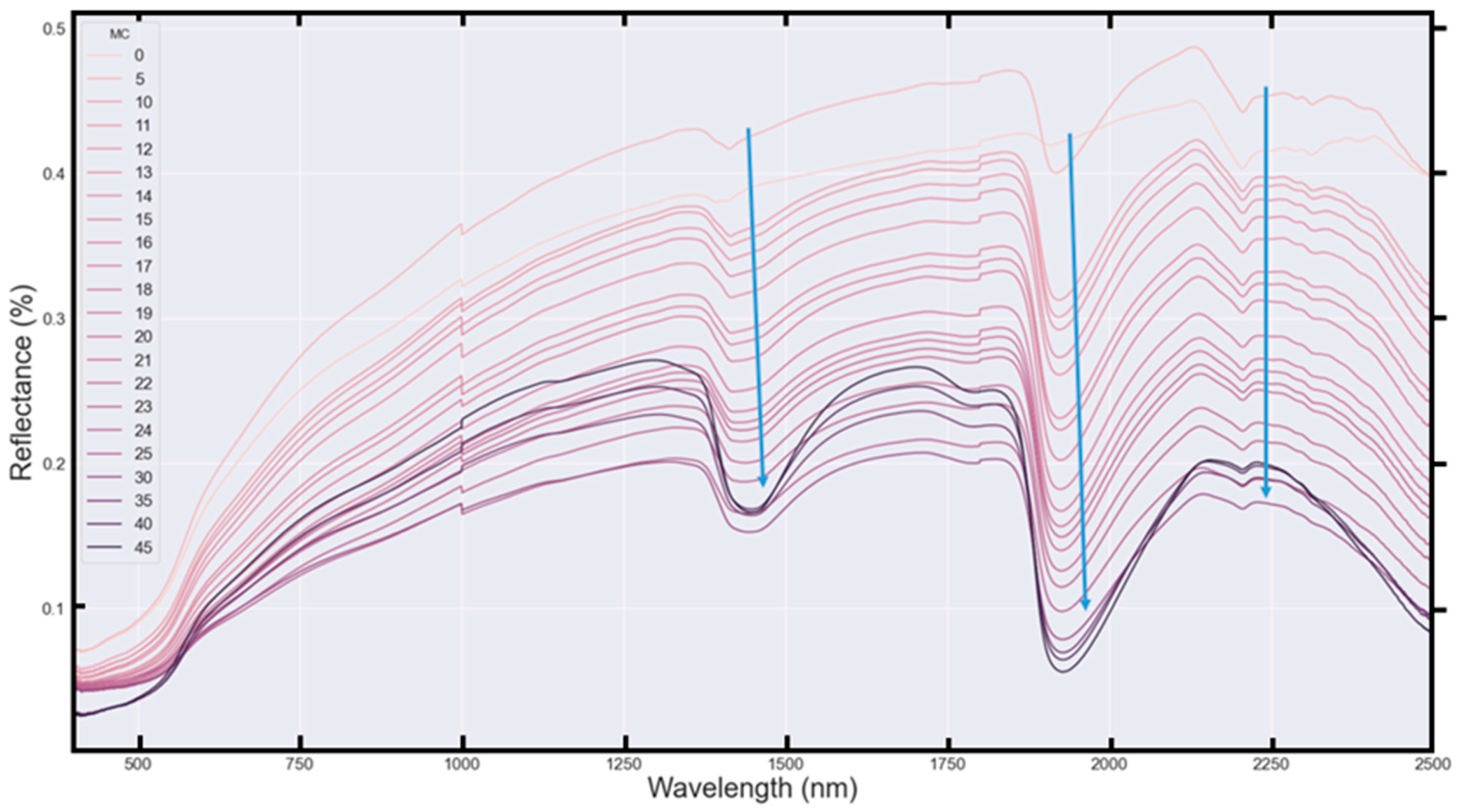
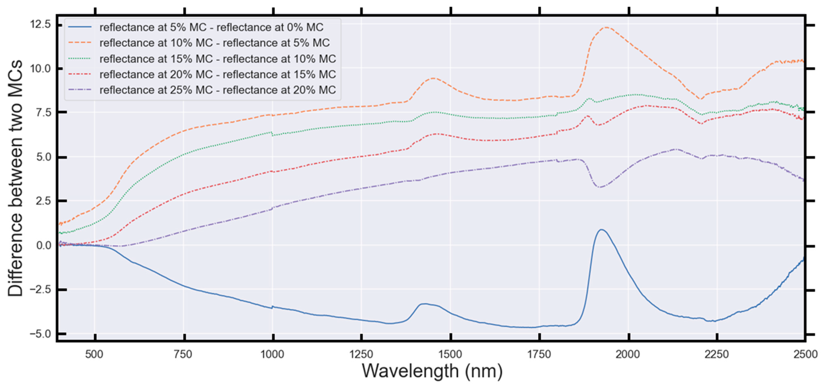
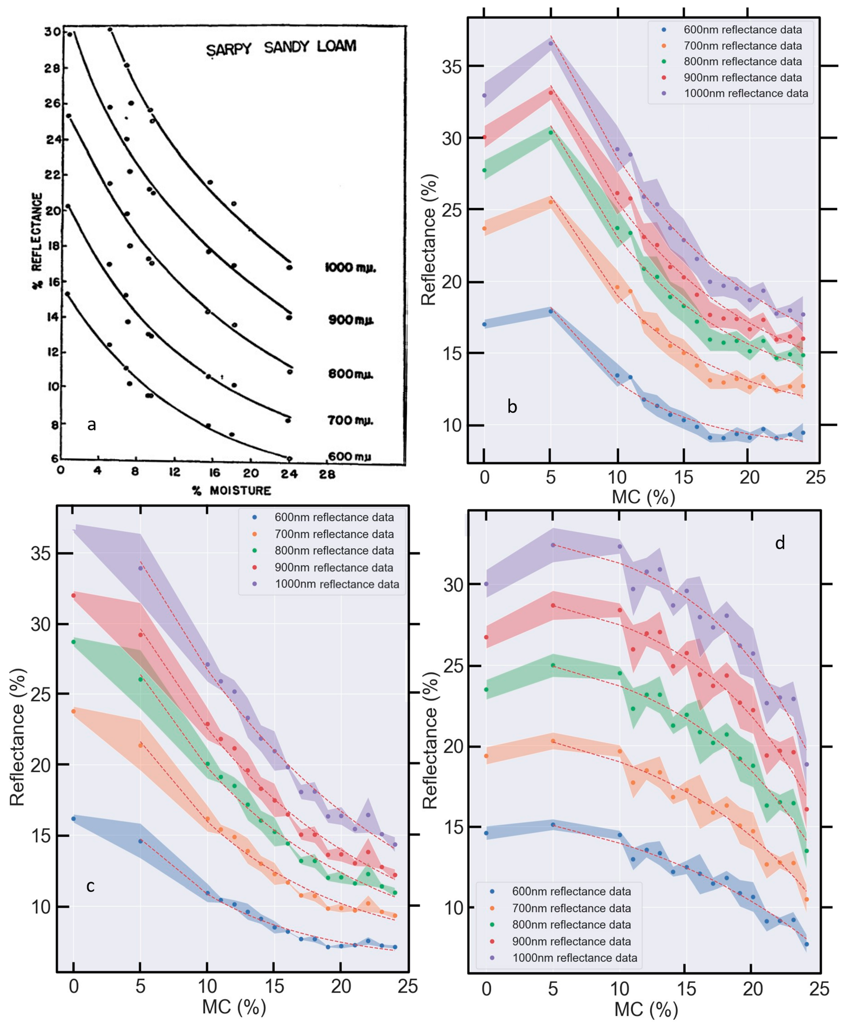
3. The Relationship between Soil MC and Reflectance—New Data
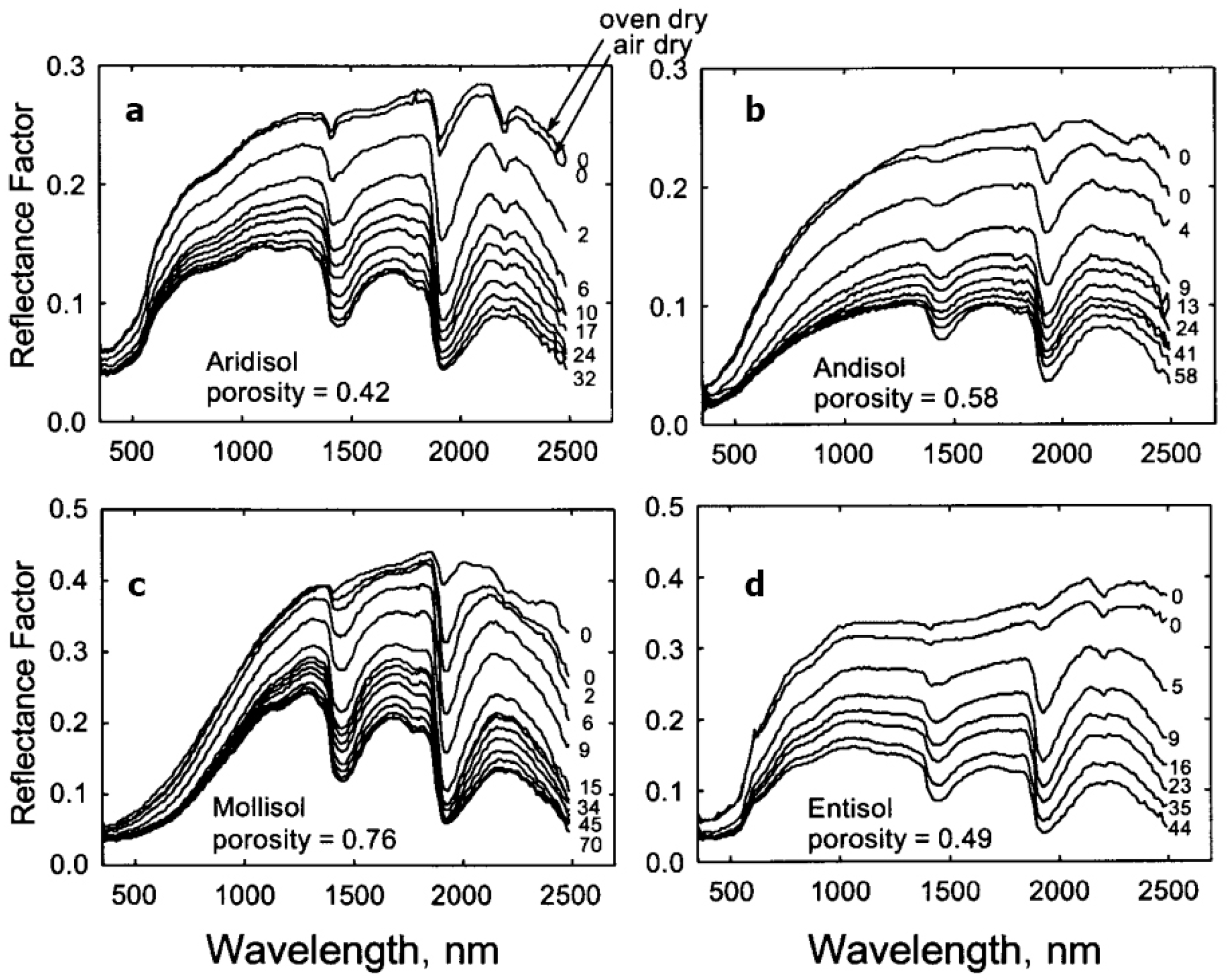
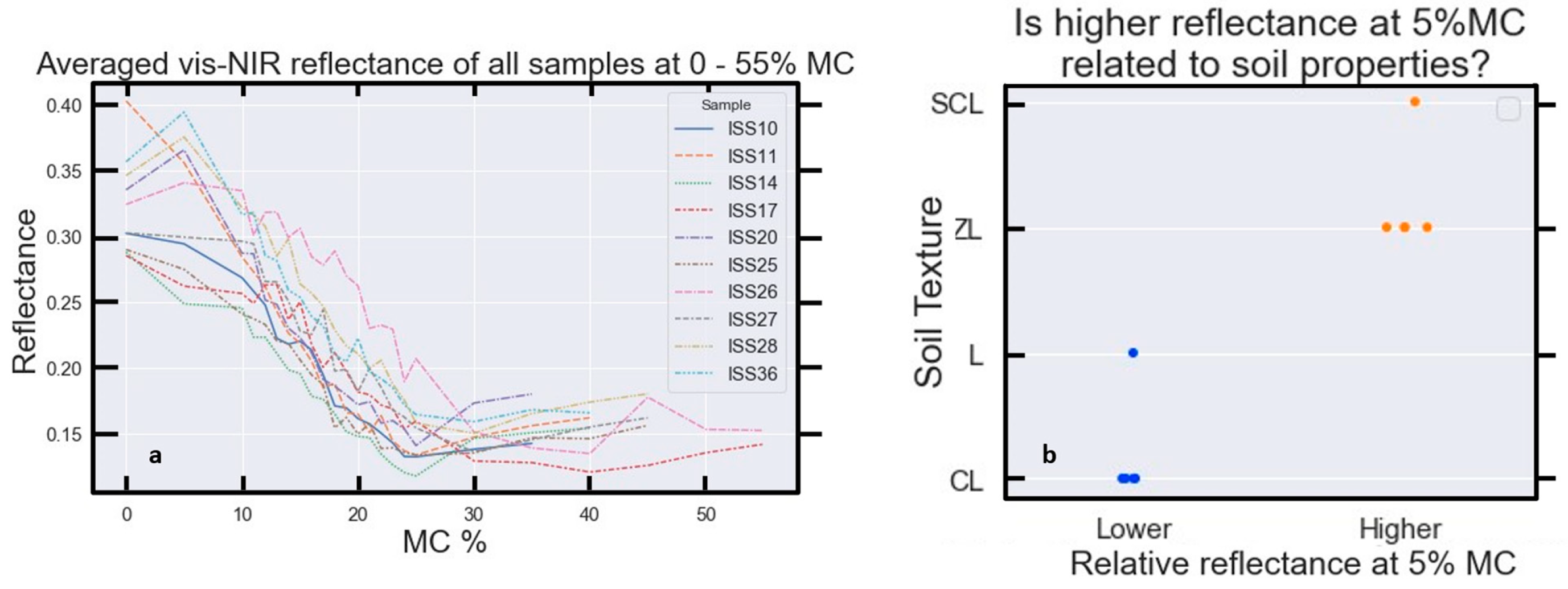
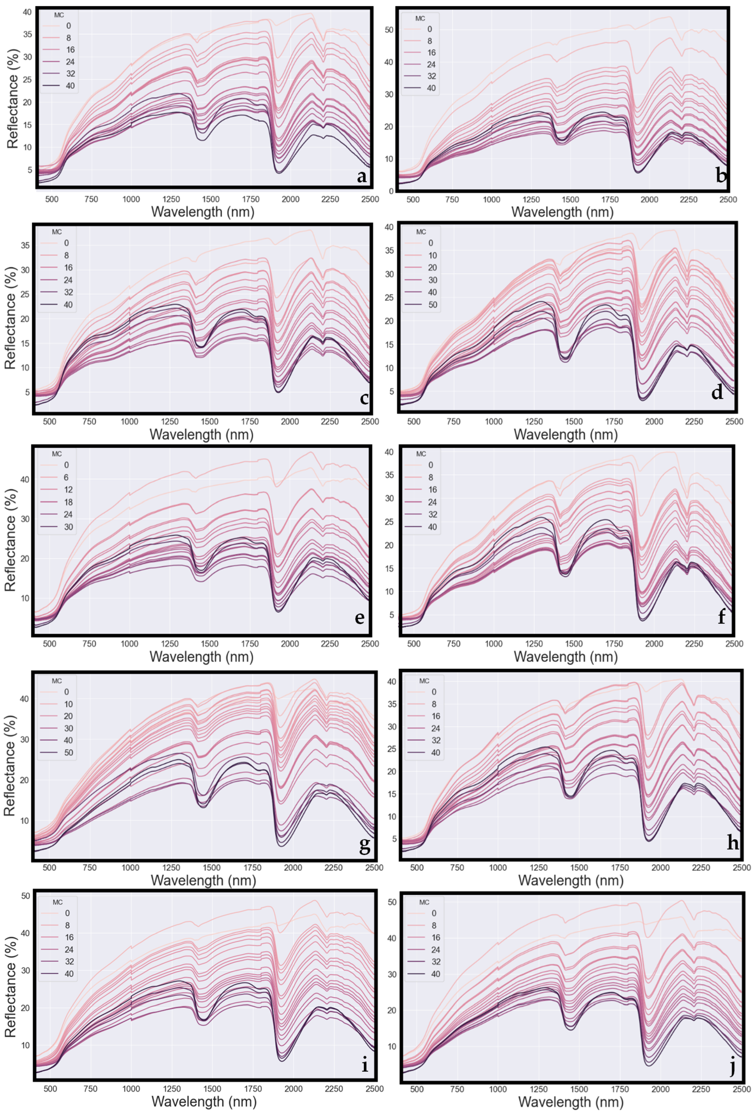
4. Spectral Intensity at Visible–NIR Wavelengths as a Function of MC for Individual Soils
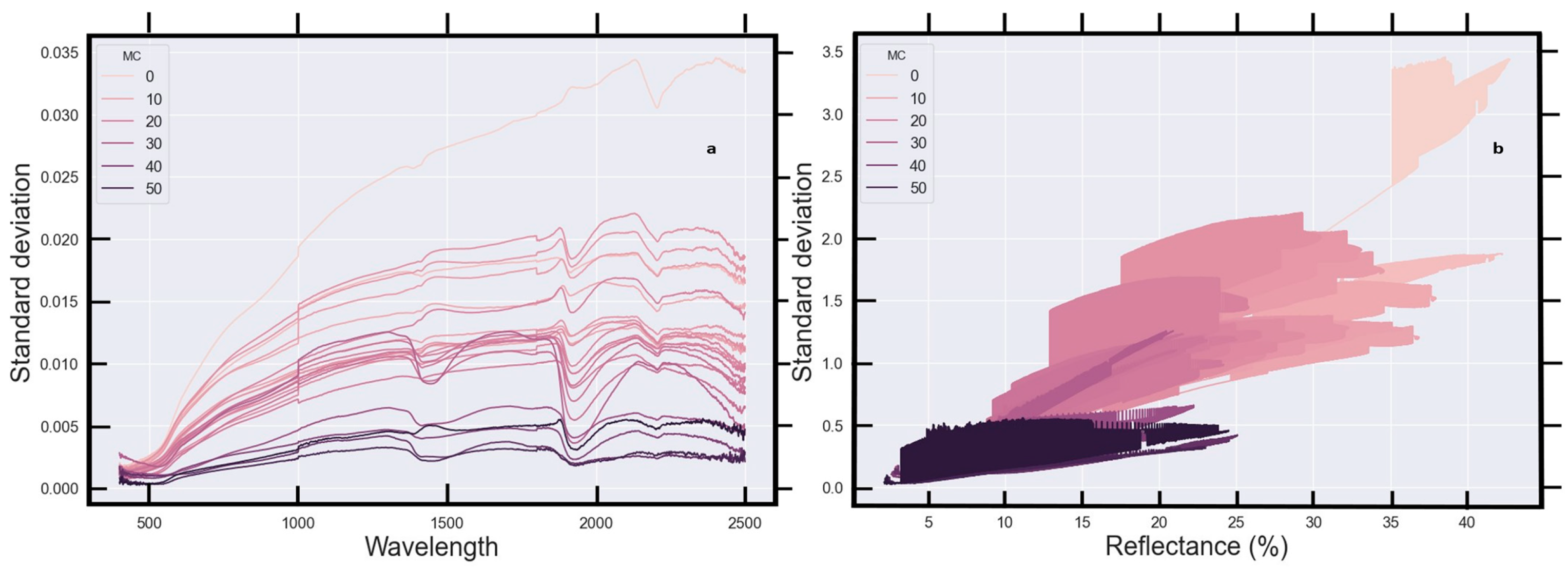
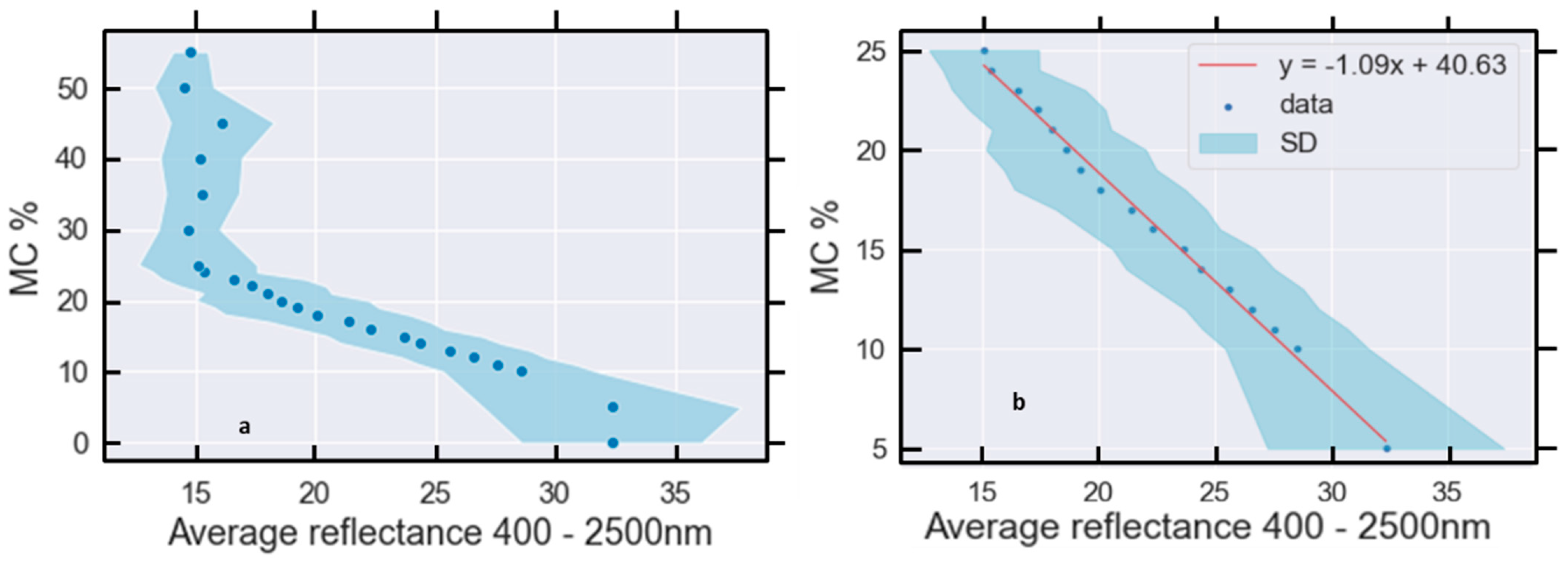
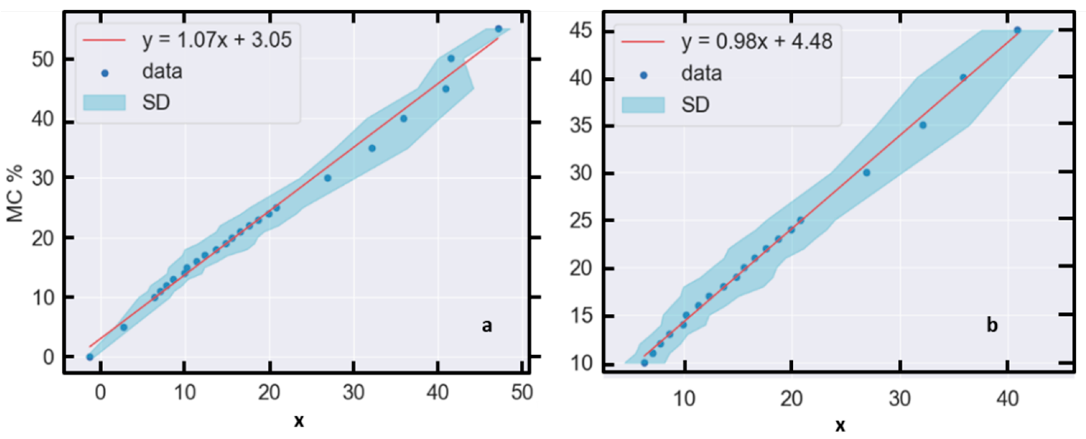
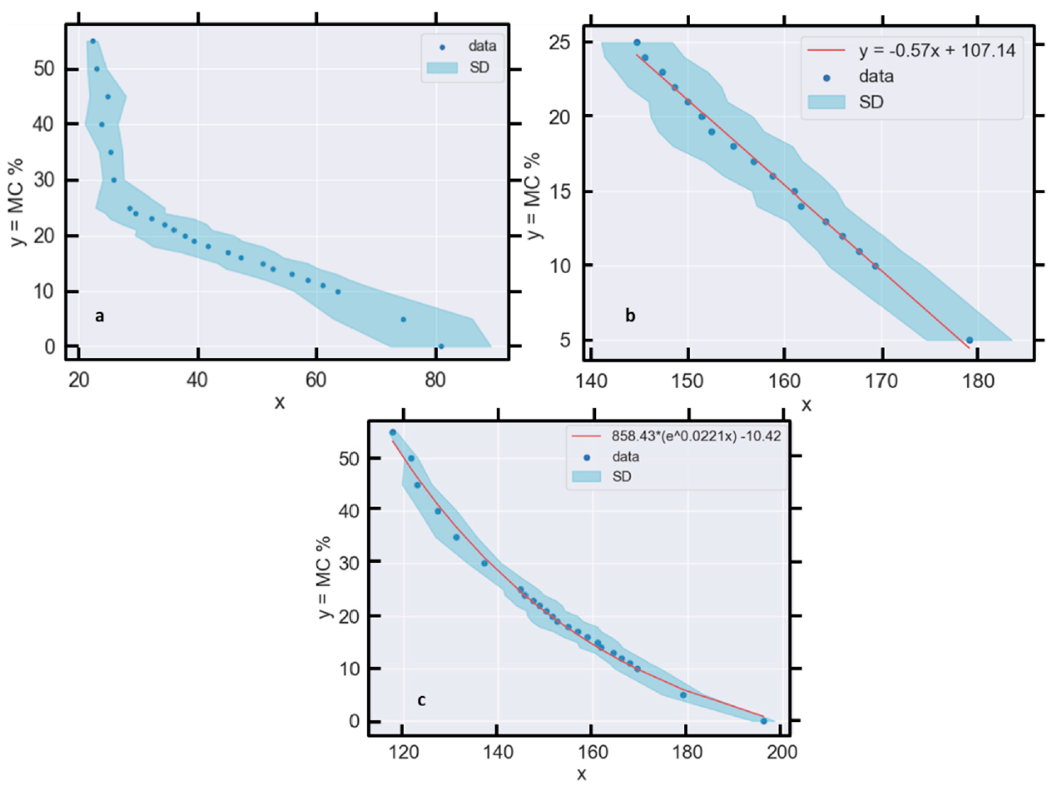
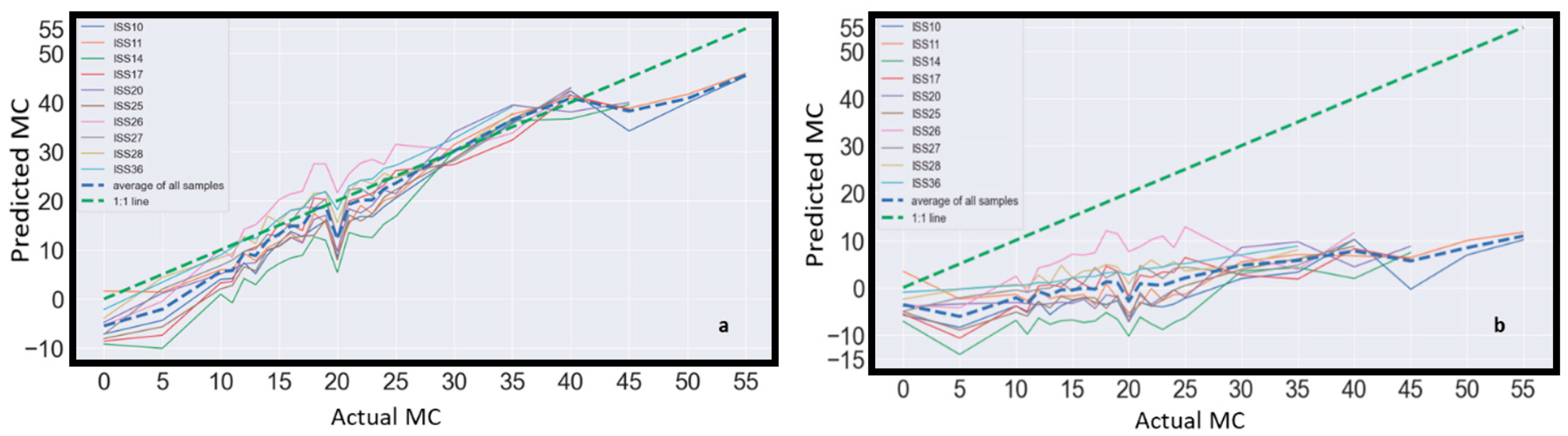
5. Averaged Reflectance vs. MC—Generalising the Relationship between Soil MC and Visible–NIR Reflectance
5.1. Averaging across All Samples
5.2. Individual Samples
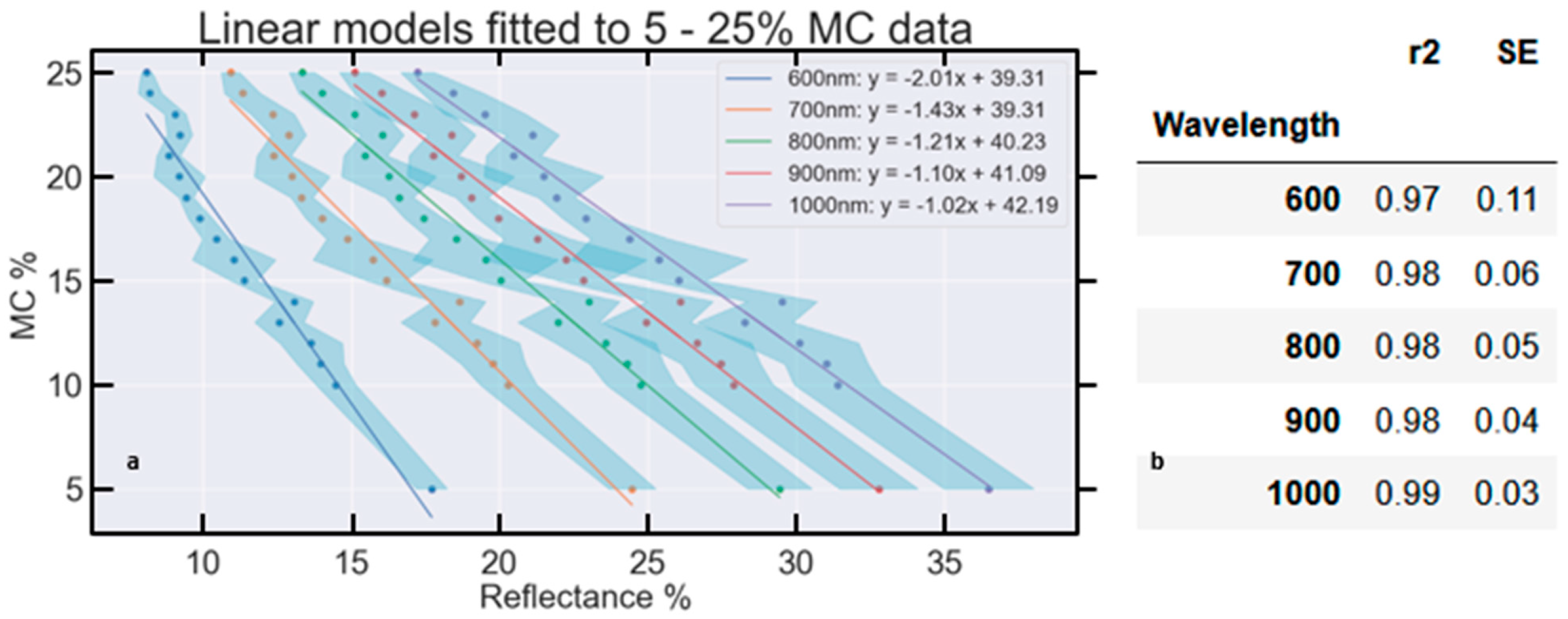
6. Relationships between Soil Reflectance and MC for Specific Wavelength Combinations
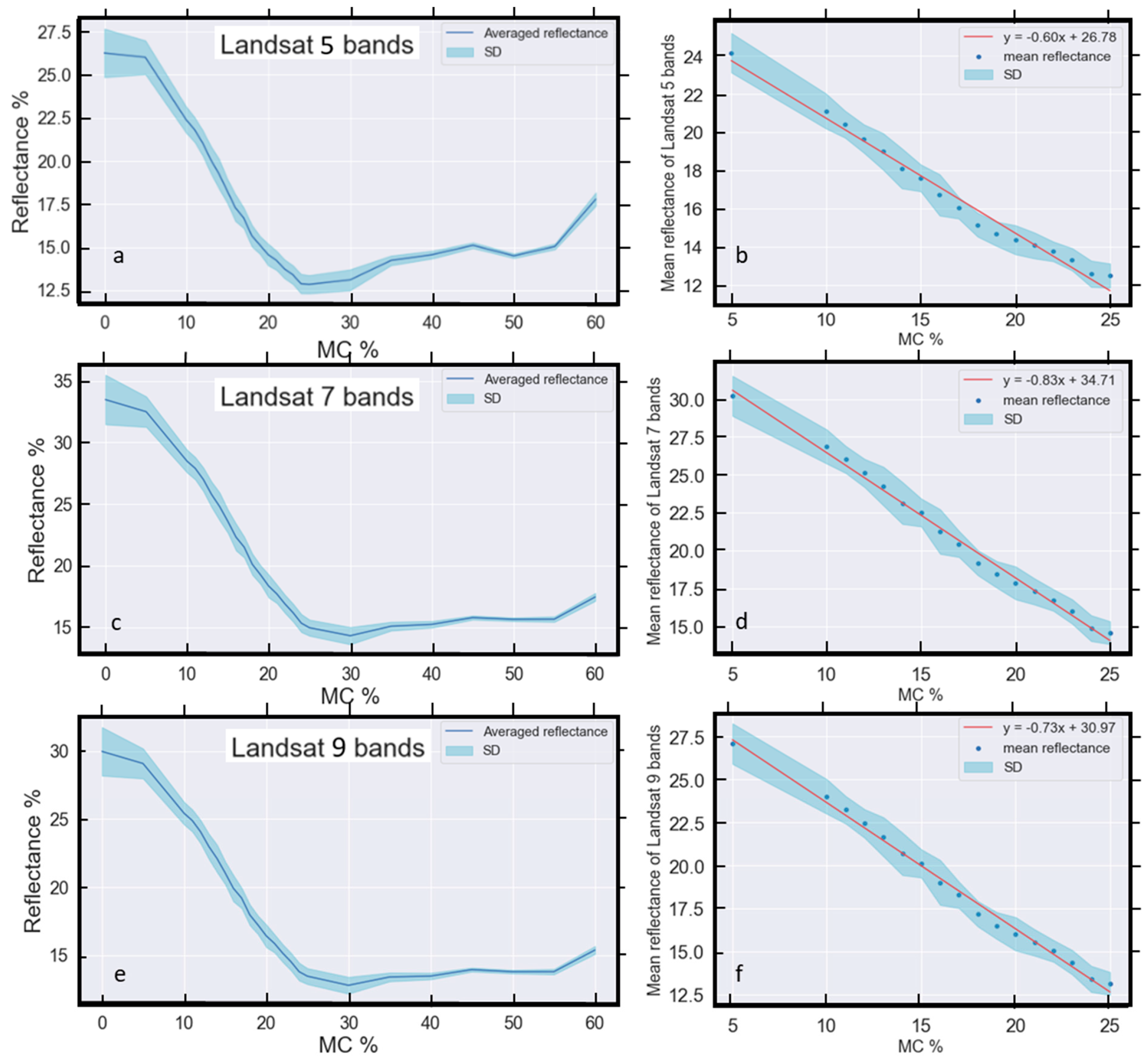
6.1. Averaged Reflectance for Several Bands vs. MC
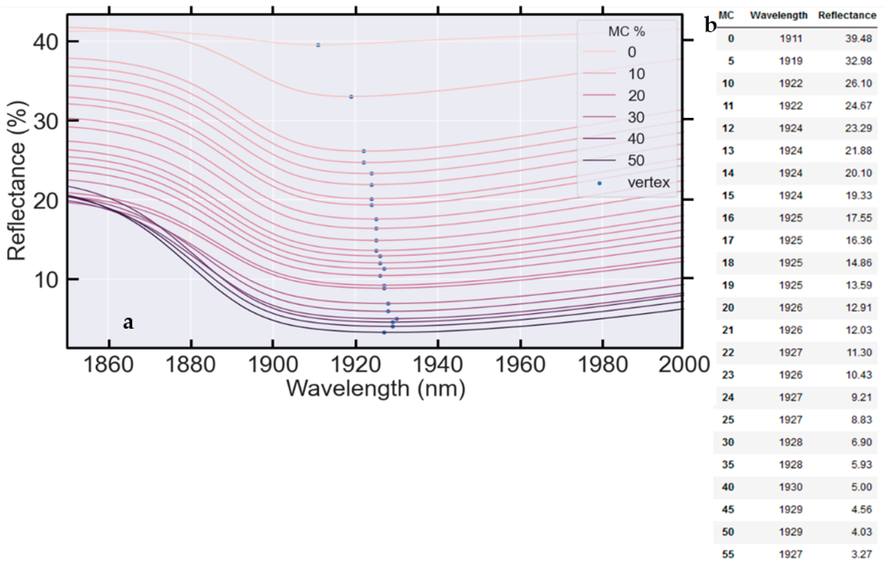
6.2. Absorption Features
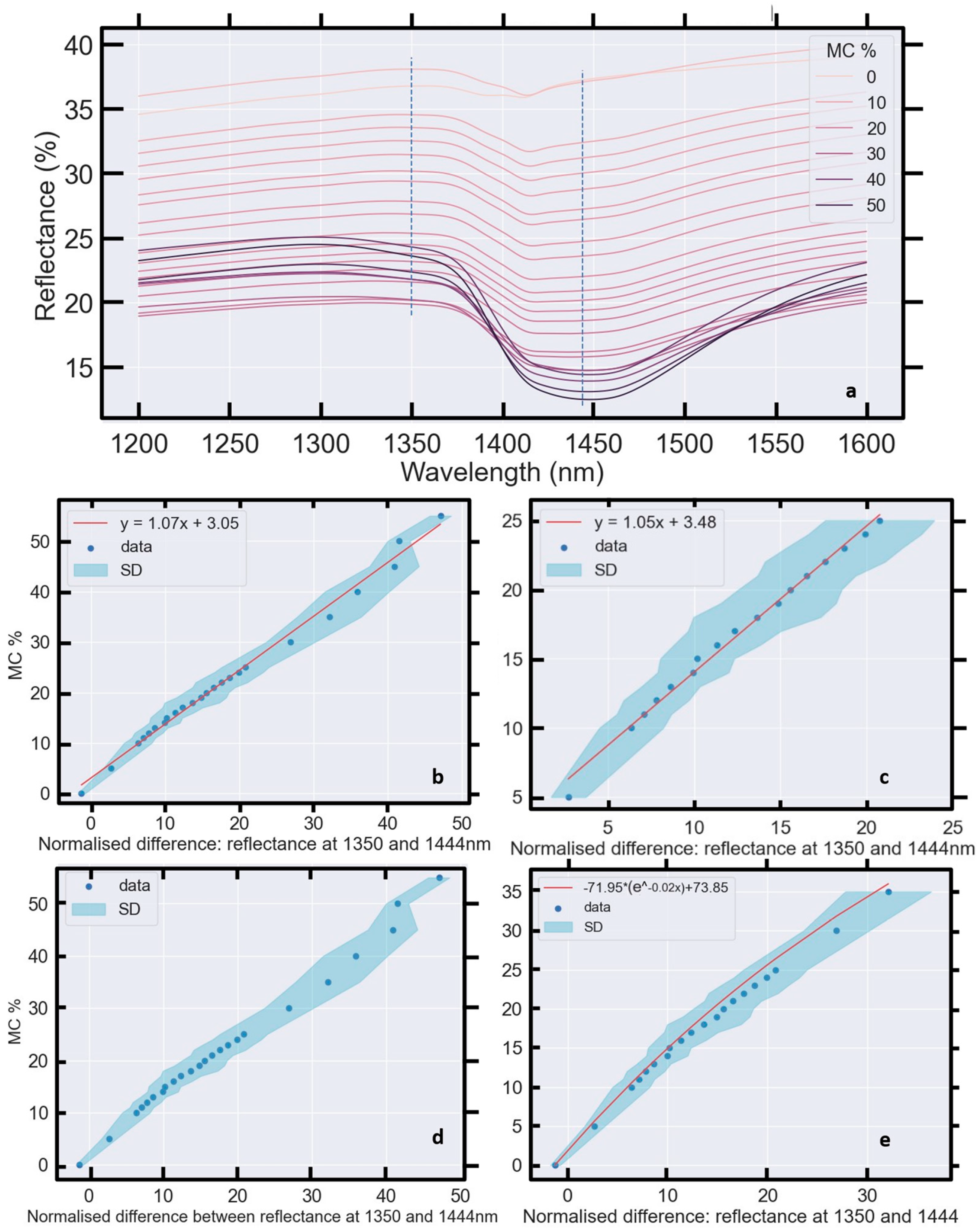
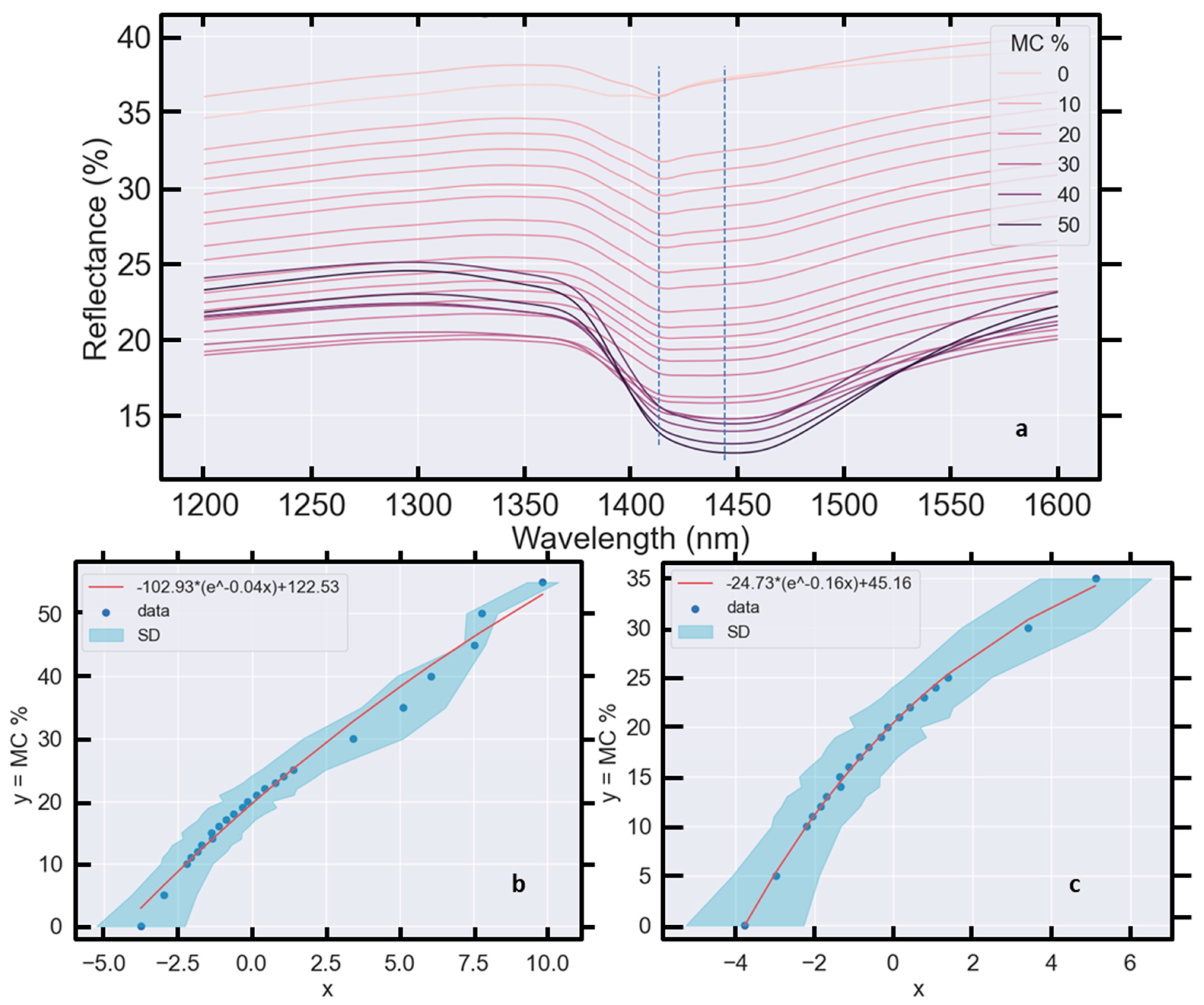
6.2.1. The 1400 nm Absorption Feature
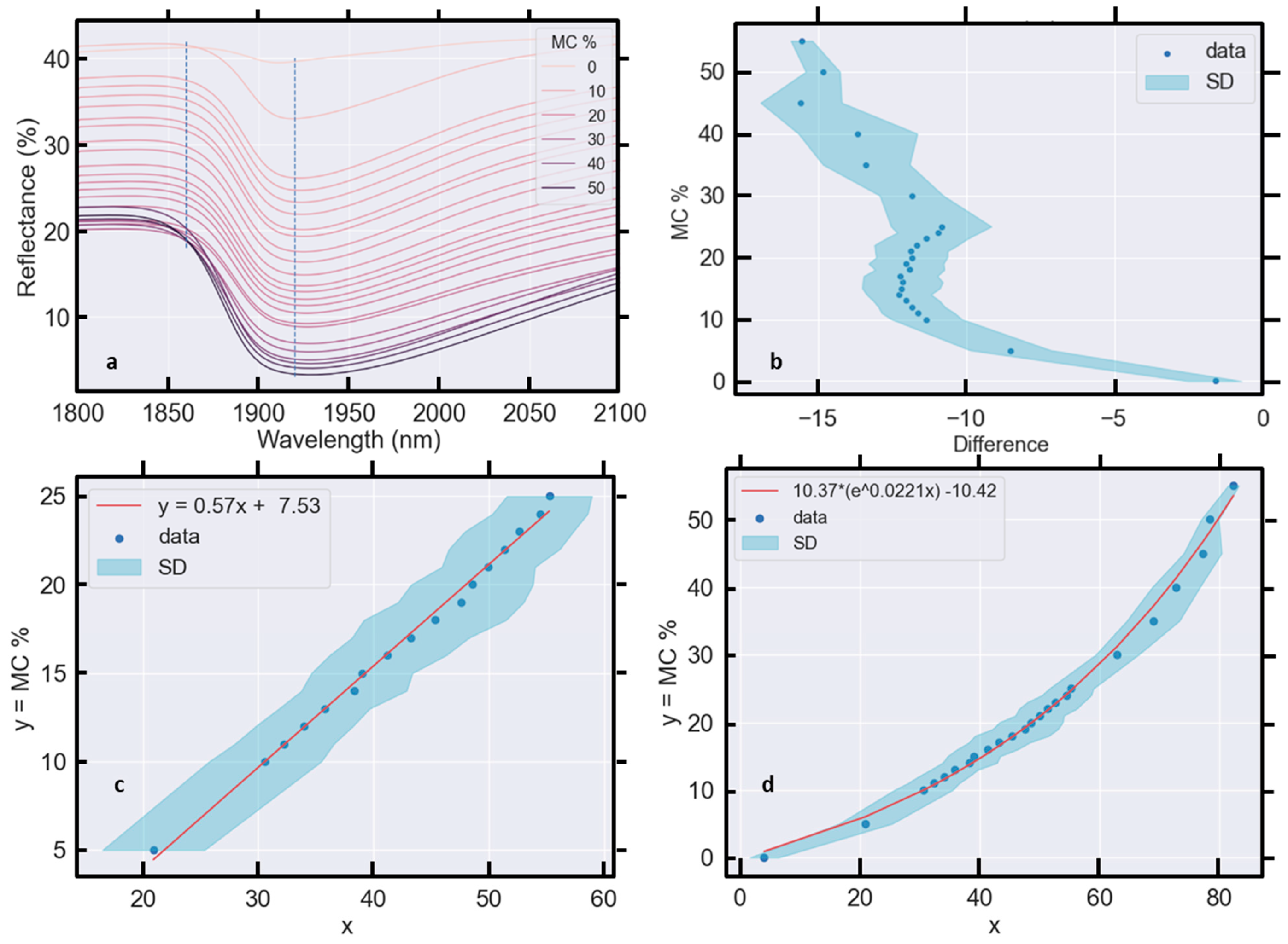
6.2.2. The 1900 nm Absorption Feature
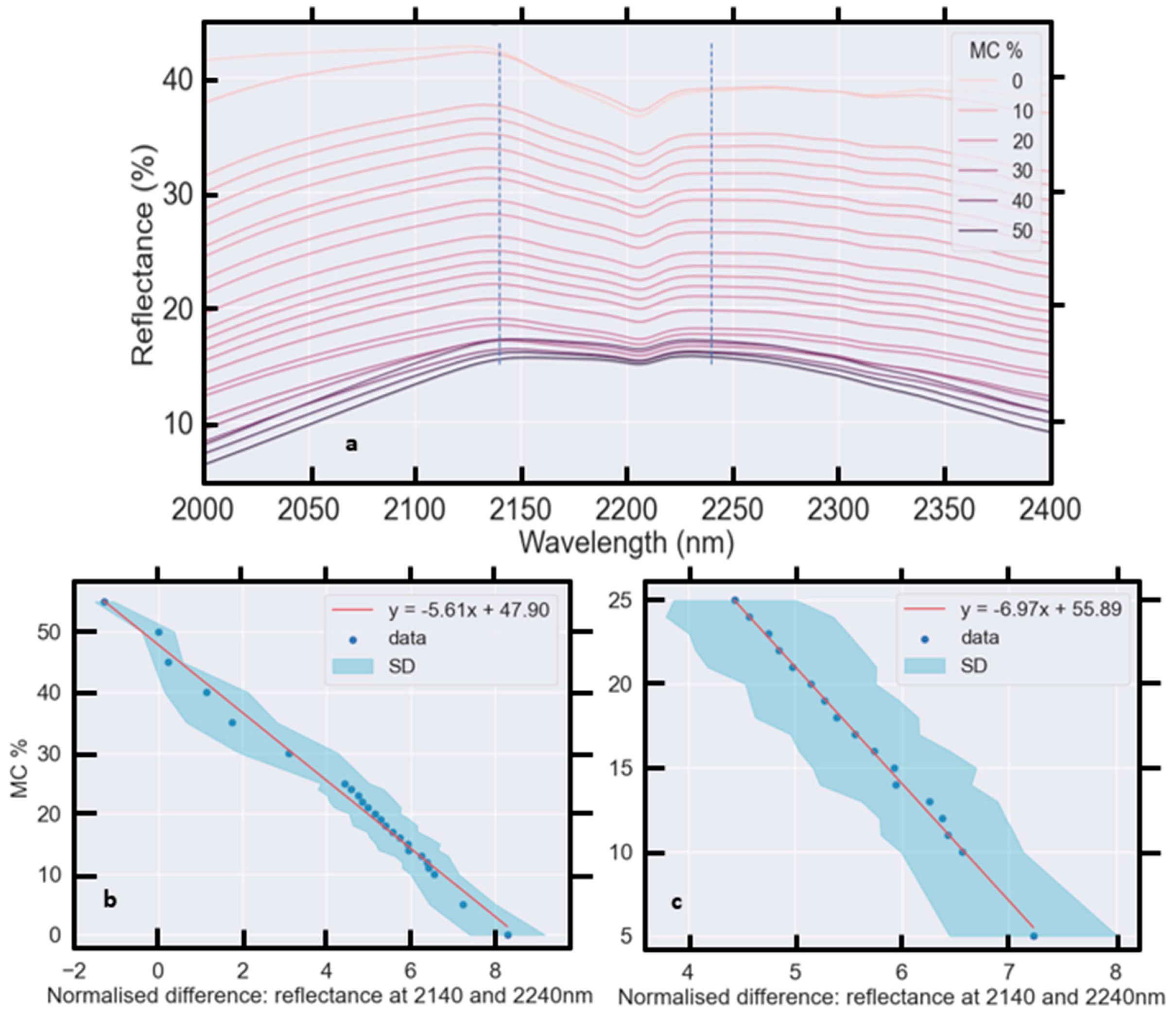
6.2.3. The 2200 nm Absorption Feature
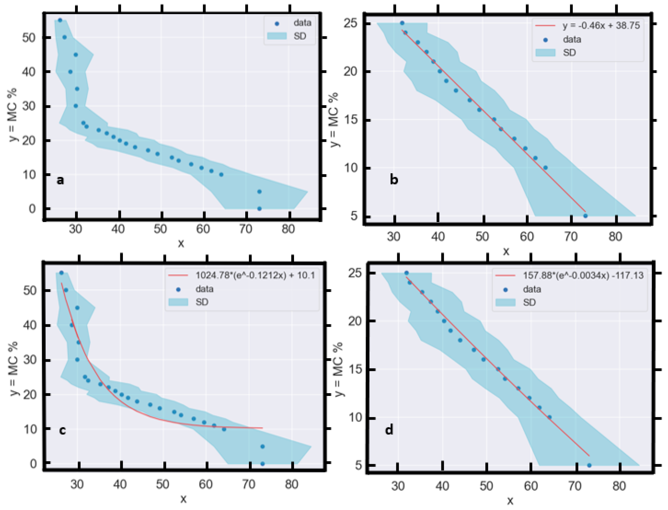
6.3. Absorption Features: Other Relative Relationships
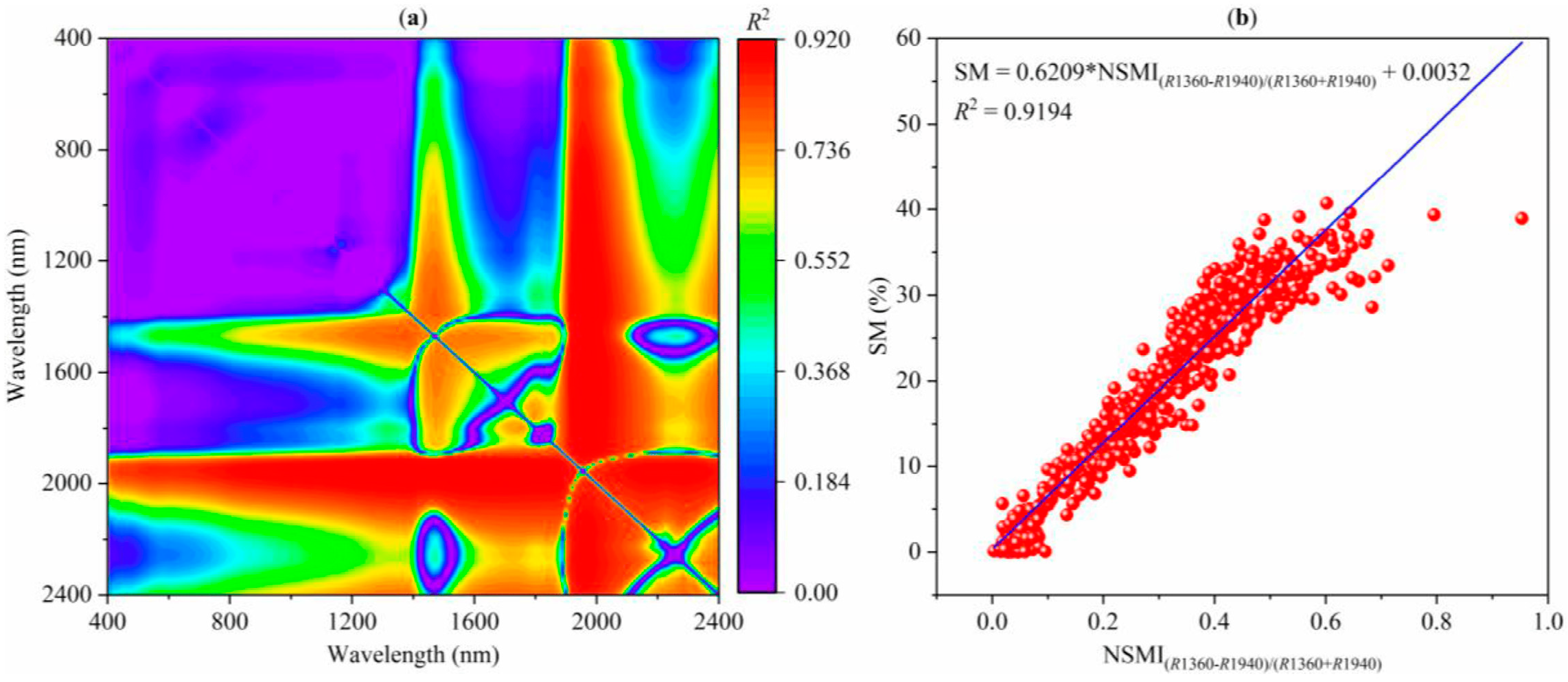
7. Normalised Soil Moisture Index
8. Discussion
8.1. Application of the Results
8.2. Future Research
8.3. Why Use Vis–NIR Data When SAR Is Available?
- Visible and NIR remotely sensed data covering much of Earth’s land surface over the past 50 years are readily available with, particularly in recent years, very high spatial (e.g., some planet satellite data are sub-meter resolution) and temporal resolution coverage. This is especially true when data products from multiple satellites are combined (e.g., Aqua and Terra MODIS satellites).
- Crucially, improved data availability makes long-term and high-temporal-resolution studies of soil moisture possible.
- Most “analysis-ready” remote sensing data products are not corrected for the effects of soil moisture. Equations used to predict soil MC can also be used to correct other remotely sensed data products for the effects of soil moisture, thereby improving prediction models for other surface, soil and atmospheric properties of interest.
- Many existing atmospheric, soil and landscape monitoring products have been developed with visible and NIR remote sensing data. Widely applicable and robust corrections for soil moisture could further improve the performance of these models.
- It is extremely valuable to understand the domain and other limits of any relationship. Prior to this review, there was a poor understanding of, and no consensus on, the limits and transferability of existing soil MC prediction models. Now, it is clear that different equations and data must be used to predict soil MC below and above 25% MC in many cases unless data indicating otherwise (e.g., Figure 21d) are available. It has also been demonstrated with analysis of the new data presented in this review that normalisation of reflectance data typically improves model performance.
8.4. Linear or Non-Linear Relationship?
- Simple linear models may be used to calculate or predict soil MC from NIR data in many cases;
- Linear correction models are widely appropriate for the correction of soil reflectance data for the effects of soil moisture.
8.5. Absorption Features
9. Conclusions
Author Contributions
Funding
Data Availability Statement
Conflicts of Interest
Appendix A. Methods
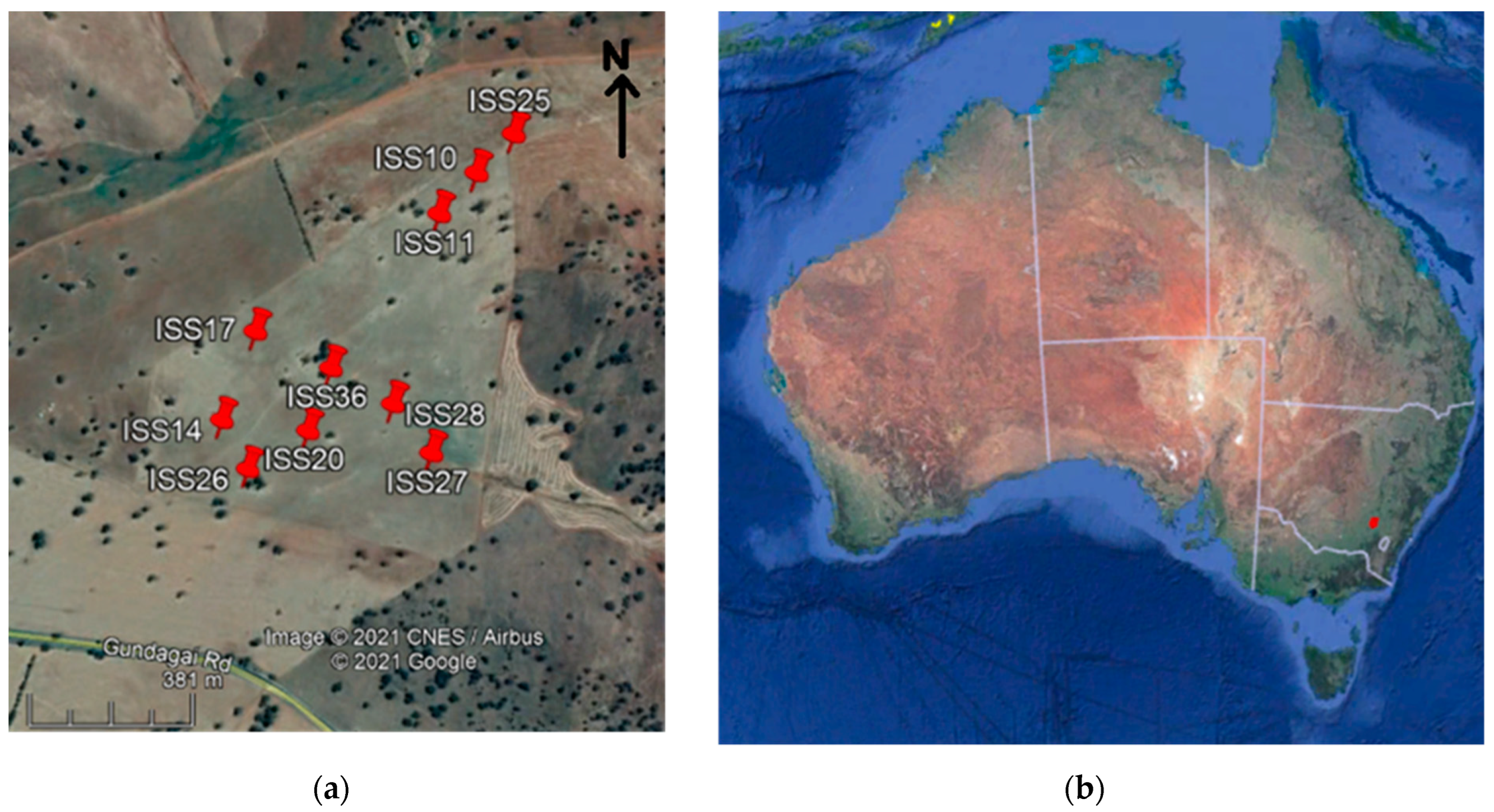
Appendix A.1. Soil Samples

| Sample | Clay % | Silt % | Sand % | Soil Texture | Organic Matter | Bulk Density |
|---|---|---|---|---|---|---|
| ISS10A | 25.41 | 18.65 | 55.93 | CL | 3.86 | 1.30 |
| ISS11A | 25.20 | 19.35 | 55.44 | CL | 4.55 | 1.26 |
| ISS14A | 22.12 | 17.05 | 60.84 | L | 3.19 | 1.36 |
| ISS17A | 25.06 | 20.89 | 54.05 | CL | 4.38 | 1.27 |
| ISS20A | 21.10 | 25.83 | 53.07 | ZL | 2.24 | 1.41 |
| ISS25A | 27.19 | 15.86 | 56.95 | CL | 3.48 | 1.33 |
| ISS26A | 18.28 | 28.56 | 53.16 | ZL | 4.26 | 1.27 |
| ISS27A | 20.24 | 6.84 | 72.93 | SCL | 3.71 | 1.34 |
| ISS28A | 18.55 | 26.02 | 55.43 | ZL | 2.83 | 1.38 |
| ISS36A | 14.47 | 27.58 | 57.94 | ZL | 3.91 | 1.31 |

Appendix A.2. Soil Moisture Addition

References
- Burk, L.; Dalgliesh, N. Estimating Plant Available Water Capacity; Grains Research and Development Corporation: Barton, Australia, 2008. [Google Scholar]
- Petronaitis, T.; Forknall, C.R.; Simpfendorfer, S.; Flavel, R.; Backhouse, D. Is There a Disease Downside to Stripper Fronts? Harvest Height Implications for Fusarium Crown Rot Management; GRDC Update; GRDC: Barton, Australia, 2022. [Google Scholar]
- Slamini, M.; Sbaa, M.; Arabi, M.; Darmous, A. Review on Partial Root-zone Drying irrigation: Impact on crop yield, soil and water pollution. Agric. Water Manag. 2022, 271, 107807. [Google Scholar] [CrossRef]
- Lankford, B.A.; Scott, C.A. The paracommons of competition for resource savings: Irrigation water conservation redistributes water between irrigation, nature, and society. Resour. Conserv. Recycl. 2023, 198, 107195. [Google Scholar] [CrossRef]
- Jha, G.; Nicolas, F.; Schmidt, R.; Suvočarev, K.; Diaz, D.; Kisekka, I.; Scow, K.; Nocco, M.A. Irrigation decision support systems (idss) for california’s water–nutrient–energy nexus. Agronomy 2022, 12, 1962. [Google Scholar] [CrossRef]
- Rasti, A.; Pineda, M.; Razavi, M. Assessment of soil moisture content measurement methods: Conventional laboratory oven versus halogen moisture analyzer. J. Soil Water Sci. 2020, 4, 151–160. [Google Scholar]
- Yaghoubi, M.; Arulrajah, A.; Horpibulsuk, S. Engineering Behaviour of a Geopolymer-stabilised High-water Content Soft Clay. Int. J. Geosynth. Ground Eng. 2022, 8, 45. [Google Scholar] [CrossRef]
- Costa, S.; Robert, D.; Kodikara, J. Climate change and geo-infrastructures. In Sustainable Civil Engineering Principles and Applications; CRC Press: Boca Raton, FL, USA, 2023; p. 217. [Google Scholar] [CrossRef]
- Barnes, E.M.; Sudduth, K.A.; Hummel, J.W.; Lesch, S.M.; Corwin, D.L.; Yang, C.; Daughtry, C.S.T.; Bausch, W.C. Remote- and Ground-Based Sensor Techniques to Map Soil Properties. Photogramm. Eng. Remote Sens. 2003, 6, 619–630. [Google Scholar] [CrossRef]
- Hossain, F.F.; Messenger, R.; Captain, G.L.; Ekin, S.; Jacob, J.D.; Taghvaeian, S.; O’Hara, J.F. Soil moisture monitoring through UAS-assisted internet of things LoRaWAN wireless underground sensors. IEEE Access 2022, 10, 102107–102118. [Google Scholar] [CrossRef]
- Glimskär, A.; Hultgren, J.; Hiron, M.; Westin, R.; Bokkers, E.A.; Keeling, L.J. Sustainable Grazing by Cattle and Sheep for Semi-Natural Grasslands in Sweden. Agronomy 2023, 13, 2469. [Google Scholar] [CrossRef]
- Orloff, A. Technology: Rural: Soil moisture probes—Where do you place them? Irrig. Aust. 2013, 29, 6–7. [Google Scholar]
- Haubrock, S.N.; Chabrillat, S.; Lemmnitz, C.; Kaufmann, H. Surface soil moisture quantification models from reflectance data under field conditions. Int. J. Remote Sens. 2008, 29, 3–29. [Google Scholar] [CrossRef]
- Cheng, M.; Jiao, X.; Liu, Y.; Shao, M.; Yu, X.; Bai, Y.; Wang, Z.; Wang, S.; Tuohuti, N.; Liu, S. Estimation of soil moisture content under high maize canopy coverage from UAV multimodal data and machine learning. Agric. Water Manag. 2022, 264, 107530. [Google Scholar] [CrossRef]
- Meng, F.; Luo, M.; Sa, C.; Wang, M.; Bao, Y. Quantitative assessment of the effects of climate, vegetation, soil and groundwater on soil moisture spatiotemporal variability in the Mongolian Plateau. Sci. Total Environ. 2022, 809, 152198. [Google Scholar] [CrossRef] [PubMed]
- Bablet, A.; Vu, P.; Jacquemoud, S.; Viallefont-Robinet, F.; Fabre, S.; Briottet, X.; Sadeghi, M.; Whiting, M.L.; Baret, F.; Tian, J. MARMIT: A multilayer radiative transfer model of soil reflectance to estimate surface soil moisture content in the solar domain (400–2500 nm). Remote Sens. Environ. 2018, 217, 1–17. [Google Scholar] [CrossRef]
- Papa, F.; Crétaux, J.-F.; Grippa, M.; Robert, E.; Trigg, M.; Tshimanga, R.M.; Kitambo, B.; Paris, A.; Carr, A.; Fleischmann, A.S. Water resources in Africa under global change: Monitoring surface waters from space. Surv. Geophys. 2023, 44, 43–93. [Google Scholar] [CrossRef] [PubMed]
- Morris, R. Spectrophotometry. Curr. Protoc. Essent. Lab. Tech. 2015, 11. [Google Scholar] [CrossRef]
- Dadi, M.; Yasir, M. Spectroscopy and Spectrophotometry: Principles and Applications for Colorimetric and Related Other Analysis. In Colorimetry; IntechOpen: London, UK, 2022; p. 81. [Google Scholar] [CrossRef]
- Tripathi, A.; Tiwari, R.K.; Tiwari, S.P. A deep learning multi-layer perceptron and remote sensing approach for soil health based crop yield estimation. Int. J. Appl. Earth Obs. Geoinf. 2022, 113, 102959. [Google Scholar] [CrossRef]
- Nocita, M.; Stevens, A.; Noon, C.; van Wesemael, B. Prediction of soil organic carbon for different levels of soil moisture using Vis-NIR spectroscopy. Geoderma 2013, 199, 37–42. [Google Scholar] [CrossRef]
- Seidel, M.; Vohland, M.; Greenberg, I.; Ludwig, B.; Ortner, M.; Thiele-Bruhn, S.; Hutengs, C. Soil moisture effects on predictive VNIR and MIR modeling of soil organic carbon and clay content. Geoderma 2022, 427, 116103. [Google Scholar] [CrossRef]
- Yu, W.; Hong, Y.; Chen, S.; Chen, Y.; Zhou, L. Comparing Two Different Development Methods of External Parameter Orthogonalization for Estimating Organic Carbon from Field-Moist Intact Soils by Reflectance Spectroscopy. Remote Sens. 2022, 14, 1303. [Google Scholar] [CrossRef]
- Sun, H.; Gao, J. A pixel-wise calculation of soil evaporative efficiency with thermal/optical remote sensing and meteorological reanalysis data for downscaling microwave soil moisture. Agric. Water Manag. 2023, 276, 108063. [Google Scholar] [CrossRef]
- Salvatore, M.R.; Barrett, J.E.; Fackrell, L.E.; Sokol, E.R.; Levy, J.S.; Kuentz, L.C.; Gooseff, M.N.; Adams, B.J.; Power, S.N.; Knightly, J.P. The Distribution of Surface Soil Moisture over Space and Time in Eastern Taylor Valley, Antarctica. Remote Sens. 2023, 15, 3170. [Google Scholar] [CrossRef]
- Weidong, L.; Baret, F.; Xingfa, G.; Qingxi, T.; Lanfen, Z.; Bing, Z. Relating soil surface moisture to reflectance. Remote Sens. Environ. 2002, 81, 238–246. [Google Scholar] [CrossRef]
- Yue, J.; Tian, J.; Tian, Q.; Xu, K.; Xu, N. Development of soil moisture indices from differences in water absorption between shortwave-infrared bands. ISPRS J. Photogramm. Remote Sens. 2019, 154, 216–230. [Google Scholar] [CrossRef]
- Lobell, D.B.; Asner, G.P. Moisture effects on soil reflectance. Soil Sci. Soc. Am. J. 2002, 66, 722–727. [Google Scholar] [CrossRef]
- Stevens, A.; Nocita, M.; Tóth, G.; Montanarella, L.; van Wesemael, B. Prediction of Soil Organic Carbon at the European Scale by Visible and Near InfraRed Reflectance Spectroscopy. PLoS ONE 2013, 8, e66409. [Google Scholar] [CrossRef]
- Hong, Y.S.; Yu, L.; Chen, Y.Y.; Liu, Y.F.; Liu, Y.L.; Liu, Y.; Cheng, H. Prediction of Soil Organic Matter by VIS-NIR Spectroscopy Using Normalized Soil Moisture Index as a Proxy of Soil Moisture. Remote Sens. 2018, 10, 28. [Google Scholar] [CrossRef]
- Mohamed, E.; Saleh, A.; Belal, A.; Gad, A.A. Application of near-infrared reflectance for quantitative assessment of soil properties. Egypt. J. Remote Sens. Space Sci. 2018, 21, 1–14. [Google Scholar] [CrossRef]
- Fabre, S.; Briottet, X.; Lesaignoux, A. Estimation of soil moisture content from the spectral reflectance of bare soils in the 0.4–2.5 µm domain. Sensors 2015, 15, 3262–3281. [Google Scholar] [CrossRef]
- Jiang, Q.; Chen, Y.; Guo, L.; Fei, T.; Qi, K. Estimating soil organic carbon of cropland soil at different levels of soil moisture using VIS-NIR spectroscopy. Remote Sens. 2016, 8, 755. [Google Scholar] [CrossRef]
- Bowers, S.A.; Hanks, R.J. Reflection of Radiant Energy from Soils. Soil Sci. 1965, 100, 130–138. [Google Scholar] [CrossRef]
- Angelopoulou, T.; Tziolas, N.; Balafoutis, A.; Zalidis, G.; Bochtis, D. Remote Sensing Techniques for Soil Organic Carbon Estimation: A Review. Remote Sens. 2019, 11, 676. [Google Scholar] [CrossRef]
- Wu, C.-Y.; Jacobson, A.R.; Laba, M.; Baveye, P.C. Alleviating moisture content effects on the visible near-infrared diffuse-reflectance sensing of soils. Soil Sci. 2009, 174, 456–465. [Google Scholar] [CrossRef]
- Nduwamungu, C.; Ziadi, N.; Tremblay, G.F.; Parent, L.-É. Near-infrared reflectance spectroscopy prediction of soil properties: Effects of sample cups and preparation. Soil Sci. Soc. Am. J. 2009, 73, 1896–1903. [Google Scholar] [CrossRef]
- Zhang, T.; Li, L.; Zheng, B. Partial least squares modeling of Hyperion image spectra for mapping agricultural soil properties. In Remote Sensing and Modeling of Ecosystems for Sustainability VI; International Society for Optics and Photonics: Bellingham, WA, USA, 2009. [Google Scholar]
- Wang, S.; Guan, K.Y.; Zhang, C.H.; Lee, D.; Margenot, A.J.; Ge, Y.F.; Peng, J.; Zhou, W.; Zhou, Q.; Huang, Y.Z. Using soil library hyperspectral reflectance and machine learning to predict soil organic carbon: Assessing potential of airborne and spaceborne optical soil sensing. Remote Sens. Environ. 2022, 271, 112914. [Google Scholar] [CrossRef]
- Whiting, M.L.; Li, L.; Ustin, S.L. Predicting water content using Gaussian model on soil spectra. Remote Sens. Environ. 2004, 89, 535–552. [Google Scholar] [CrossRef]
- Viscarra Rossel, R.A.; Behrens, T.; Ben-Dor, E.; Brown, D.J.; Dematte, J.A.M.; Shepherd, K.D.; Shi, Z.; Stenberg, B.; Stevens, A.; Adamchuk, V.; et al. A global spectral library to characterise the world’s soil. Earth-Sci. Rev. 2016, 1, 198–230. [Google Scholar] [CrossRef]
- Zhang, Z.; Ding, J.; Wang, J.; Ge, X. Prediction of soil organic matter in northwestern China using fractional-order derivative spectroscopy and modified normalized difference indices. Catena 2020, 185, 104257. [Google Scholar] [CrossRef]
- Minasny, B.; McBratney, A.B.; Bellon-Maurel, V.; Roger, J.-M.; Gobrecht, A.; Ferrand, L.; Joalland, S. Removing the effect of soil moisture from NIR diffuse reflectance spectra for the prediction of soil organic carbon. Geoderma 2011, 167, 118–124. [Google Scholar] [CrossRef]
- Roudier, P.; Hedley, C.; Lobsey, C.; Rossel, R.V.; Leroux, C. Evaluation of two methods to eliminate the effect of water from soil vis–NIR spectra for predictions of organic carbon. Geoderma 2017, 296, 98–107. [Google Scholar] [CrossRef]
- Mouazen, A.; De Baerdemaeker, J.; Ramon, H. Effect of wavelength range on the measurement accuracy of some selected soil constituents using visual-near infrared spectroscopy. J. Near Infrared Spectrosc. 2006, 14, 189–199. [Google Scholar] [CrossRef]
- Ishida, T.; Ando, H.; Fukuhara, M. Estimation of complex refractive index of soil particles and its dependence on soil chemical properties. Remote Sens. Environ. 1991, 38, 173–182. [Google Scholar] [CrossRef]
- Ben-Dor, E. Quantitative Remote Sensing of Soil Properties. Adv. Agron. 2002, 75, 173–243. [Google Scholar]
- Člupek, M.; Matějka, P.; Volka, K. Noise reduction in Raman spectra: Finite impulse response filtration versus Savitzky–Golay smoothing. J. Raman Spectrosc. 2007, 38, 1174–1179. [Google Scholar] [CrossRef]
- Li, Y.; Liu, S.; Liao, Z.; He, C. Comparison of two methods for estimation of soil water content from measured reflectance. Can. J. Soil Sci. 2012, 92, 845–857. [Google Scholar] [CrossRef]
- Liu, H.J.; Zhang, Y.Z.; Zhang, X.L.; Zhang, B.; Kai Shan, S.; Zong Ming, W.; Na, T. Quantitative analysis of moisture effect on black soil reflectance. Pedosphere 2009, 19, 532–540. [Google Scholar] [CrossRef]
- Condit, H. Application of characteristic vector analysis to the spectral energy distribution of daylight and the spectral reflectance of American soils. Appl. Opt. 1972, 11, 74–86. [Google Scholar] [CrossRef] [PubMed]
- Stenberg, B.; Viscarra Rossel, R.A.; Mouazen, A.M.; Wetterlind, J. Visible and Near Infrared Spectroscopy in Soil Science. In Advances in Agronomy; Elsevier: Amsterdam, The Netherlands; Academic Press: Cambridge, MA, USA, 2010; Volume 107, pp. 163–215. [Google Scholar]
- Philpot, W. Spectral Reflectance of Wetted Soils. In Proceedings of the Art, Science and Applications of Reflectance Spectroscopy (ASARS), Boulder, CO, USA, 23–25 February 2010; pp. 1–12. [Google Scholar]
- Demattê, J.A.; Campos, R.C.; Alves, M.C.; Fiorio, P.R.; Nanni, M.R. Visible–NIR reflectance: A new approach on soil evaluation. Geoderma 2004, 121, 95–112. [Google Scholar] [CrossRef]
- Liu, W.; Baret, F.; Gu, X.; Zhang, B.; Tong, Q.; Zheng, L. Evaluation of methods for soil surface moisture estimation from reflectance data. Int. J. Remote Sens. 2003, 24, 2069–2083. [Google Scholar] [CrossRef]
- Bogrekci, I.; Lee, W. Effects of soil moisture content on absorbance spectra of sandy soils in sensing phosphorus concentrations using UV-VIS-NIR spectroscopy. Trans. Am. Soc. Agric. Biol. Eng. 2006, 49, 1175–1180. [Google Scholar] [CrossRef]
- Tan, Y.; Jiang, Q.G.; Yu, L.F.; Liu, H.X.; Zhang, B. Reducing the Moisture Effect and Improving the Prediction of Soil Organic Matter With VIS-NIR Spectroscopy in Black Soil Area. IEEE Access 2021, 9, 5895–5905. [Google Scholar] [CrossRef]
- Campbell, P.K.E.; Middleton, E.M.; Thome, K.J.; Kokaly, R.F.; Huemmrich, K.F.; Lagomasino, D.; Novick, K.A.; Brunsell, N.A. EO-1 hyperion reflectance time series at calibration and validation sites: Stability and sensitivity to seasonal dynamics. IEEE J. Sel. Top. Appl. Earth Obs. Remote Sens. 2013, 6, 276–290. [Google Scholar] [CrossRef]
- Dotto, A.C.; Dalmolin, R.S.D.; ten Caten, A.; Grunwald, S. A systematic study on the application of scatter-corrective and spectral-derivative preprocessing for multivariate prediction of soil organic carbon by Vis-NIR spectra. Geoderma 2018, 314, 262–274. [Google Scholar] [CrossRef]
- Demattê, J.A.; da Silva Terra, F. Spectral pedology: A new perspective on evaluation of soils along pedogenetic alterations. Geoderma 2014, 217, 190–200. [Google Scholar] [CrossRef]
- Ben-Dor, E.; Banin, A. Near-infrared analysis as a rapid method to simultaneously evaluate several soil properties. Soil Sci. Soc. Am. J. 1995, 59, 364–372. [Google Scholar] [CrossRef]
- Soriano-Disla, J.M.; Janik, L.J.; Viscarra Rossel, R.A.; Macdonald, L.M.; McLaughlin, M.J. The Performance of Visible, Near-, and Mid-Infrared Reflectance Spectroscopy for Prediction of Soil Physical, Chemical, and Biological Properties. Appl. Spectrosc. Rev. 2014, 49, 139–186. [Google Scholar] [CrossRef]
- Wang, J.; Tiyip, T.; Ding, J.; Zhang, D.; Liu, W.; Wang, F.; Tashpolat, N. Desert soil clay content estimation using reflectance spectroscopy preprocessed by fractional derivative. PLoS ONE 2017, 12, e0184836. [Google Scholar] [CrossRef] [PubMed]
- Ding, J.; Yang, A.; Wang, J.; Sagan, V.; Yu, D. Machine-learning-based quantitative estimation of soil organic carbon content by VIS/NIR spectroscopy. PeerJ 2018, 6, e5714. [Google Scholar] [CrossRef] [PubMed]
- McGuirk, S.; Cairns, I. Soil Moisture Remote Sensing with Multispectral and Visible NIR Remote Sensing. ISPRS Ann. Photogramm. Remote Sens. Spat. Inf. Sci. 2022, 3, 447–453. [Google Scholar] [CrossRef]
- Chen, F.; Lasaponara, R.; Masini, N. An overview of satellite synthetic aperture radar remote sensing in archaeology: From site detection to monitoring. J. Cult. Herit. 2017, 23, 5–11. [Google Scholar] [CrossRef]
- Merzouki, A.; McNairn, H.; Powers, J.; Friesen, M. Synthetic aperture radar (SAR) compact polarimetry for soil moisture retrieval. Remote Sens. 2019, 11, 2227. [Google Scholar] [CrossRef]
- Munda, M.K.; Parida, B.R. Soil moisture modeling over agricultural fields using C-band synthetic aperture radar and modified Dubois model. Appl. Geomat. 2023, 15, 97–108. [Google Scholar] [CrossRef]
- Office of Environment and Heritage. Soil Survey Standard Test Method—Soil Moisture Content; Office of Environment and Heritage: Broken Hill, Australia, 1990. [Google Scholar]


| Landsat | Band 1 | Band 2 | Band 3 | Band 4 | Band 5 | Band 6 | Band 7 | Equation No. |
|---|---|---|---|---|---|---|---|---|
| 5 (TM) | 450–520 | 520–600 | 630–690 | 760–900 | 1550–1750 | NA | NA | (3) |
| 7 (ETM+) | 450–520 | 520–600 | 630–690 | 770–900 | 1550–1750 | NA | NA | (4) |
| 9 | 450–520 | 520–600 | 630–690 | 770–900 | 1550–1750 | 1570–1650 | 2110–2290 | (5) |
Disclaimer/Publisher’s Note: The statements, opinions and data contained in all publications are solely those of the individual author(s) and contributor(s) and not of MDPI and/or the editor(s). MDPI and/or the editor(s) disclaim responsibility for any injury to people or property resulting from any ideas, methods, instructions or products referred to in the content. |
© 2024 by the authors. Licensee MDPI, Basel, Switzerland. This article is an open access article distributed under the terms and conditions of the Creative Commons Attribution (CC BY) license (https://creativecommons.org/licenses/by/4.0/).
Share and Cite
McGuirk, S.L.; Cairns, I.H. Relationships between Soil Moisture and Visible–NIR Soil Reflectance: A Review Presenting New Analyses and Data to Fill the Gaps. Geotechnics 2024, 4, 78-108. https://doi.org/10.3390/geotechnics4010005
McGuirk SL, Cairns IH. Relationships between Soil Moisture and Visible–NIR Soil Reflectance: A Review Presenting New Analyses and Data to Fill the Gaps. Geotechnics. 2024; 4(1):78-108. https://doi.org/10.3390/geotechnics4010005
Chicago/Turabian StyleMcGuirk, Savannah L., and Iver H. Cairns. 2024. "Relationships between Soil Moisture and Visible–NIR Soil Reflectance: A Review Presenting New Analyses and Data to Fill the Gaps" Geotechnics 4, no. 1: 78-108. https://doi.org/10.3390/geotechnics4010005