Modelling of Truck Tire–Rim Slip on Sandy Loam Using Advanced Computational Techniques

Abstract

Vehicles often experience low tire pressures and high torques in off-road operations, making tire–rim slip likely. Tire–rim slip is undesirable relative rotation between the tire and rim, which, in this study, is measured by the relative tire–rim slip rate. There is little research on the effect of different terrains on tire–rim slip despite its significance for off-road driving; therefore, this topic was explored through Finite Element Analysis (FEA) simulations. An upland sandy loam soil was modelled and calibrated using Smoothed-Particle Hydrodynamics (SPH), and then a Regional Haul Drive (RHD) truck tire was simulated driving over this terrain, with a drawbar load added to increase drive torque. To examine their effects, five parameters were changed: tire–rim friction coefficient, longitudinal wheel speed, drawbar load, vertical load, and inflation pressure. The simulations showed that increasing the tire–rim friction coefficient and the inflation pressure decreased the tire–rim slip while increasing the vertical and drawbar loads increased the tire–rim slip. Varying the longitudinal wheel speed had no significant effect. Tire–rim slip was more likely to occur on the soil because it happened at lower drawbar loads on the soil than on the hard surface. These research results increased knowledge of tire–rim slip mechanics and provided a foundation for exploring tire–rim slip on other terrains, such as clays or sands.

1. Introduction

Tire and soil modelling has a long history in the field of automotive engineering. However, one specific area that has seen somewhat less attention and is therefore worth studying is the tire–rim interface. This study will focus particularly on the influence of terrain on relative motion at the tire–rim interface, also known as tire–rim slip.

The importance of tire–rim slip for off-road driving is reflected by the existence of a tire–rim slip test procedure, ASTM F2803, originally developed by the military for qualifying the tires of off-road vehicles [1,2]. Furthermore, several manufacturers have released service bulletins for diagnosing tire–rim slip, indicating that it is an important fault condition affecting vehicle performance [3,4]. Therefore, it would be beneficial to extend previous work on simulating tire–rim slip on a hard surface [5] to include the effects of a different terrain on the tire–rim slip, namely upland sandy loam. Useful simulation results will require the latest modelling methods for the tire, contact, and soil models; therefore, a review of the development of each of these areas is in order.

Early tire models such as the Magic Formula tire model by Pacejka [6], the string tire model [7], and the work on terrain modelling by Wong [8] attempted to combine both analytical equations and empirical data to create efficient and simple mathematical models. However, since the beginning of the 21st century, more advanced and powerful computer-enabled numerical models have grown in popularity; therefore, they will be the main focus of this brief literature review.

One of the first applications of Finite Element Analysis (FEA) for modelling tires was on space shuttle landing gear [9]. Those efforts used a rather simple tire composed of nonlinear shell elements, with a novel internal energy formulation developed to represent rubber hysteresis during the loading/unloading of a static tire. Later, FEA models were created specifically for passenger vehicle tires in order to simulate crash scenarios and improve crash safety [10,11]. However, researchers recognized that tires made from a single layer of shell or membrane elements, while very efficient computationally, had unrealistic deformation behaviours such as cupping and mesh entanglement [10,11]. The solution was to create a more detailed tire model using different types of elements like beams and solids to represent the different tire parts, such as the bead, plies, and tread. This was implemented successfully in multiple studies [10,11,12,13,14], with each researcher using a slightly different approach.

Of particular relevance for the present research is previous FEA work on the tire–rim interaction. This is a relatively under-researched area of tire modelling, and to the authors’ knowledge, there have been fewer published developments in this area compared to others, such as rubber materials [15,16] or tire-road friction [17,18]. One reason for the low number of publications is that in most driving conditions, the likelihood and influence of tire–rim slip is low, assuming that the tires are properly mounted and inflated; thus, it is computationally expedient to assume a rigid connection and focus the simulation resources on other, more relevant parts of the tire model. In multiple current studies, the variable nature of the tire–rim interaction is ignored [14,19,20], and a fixed or tied connection between the tire and rim nodes is used instead of a contact algorithm. However, in some cases, this limitation and the possibility for improvement with a more detailed contact definition are acknowledged [19]. Using a tire–rim contact algorithm, even a simple one, therefore advances the field.

One of the first uses of FEA for studying the tire–rim interface was for tire and bead fitment [21]. It was found that different factors, such as the inflation pressure, rim profile, and bead shape, had an impact on the total holding friction between the tire and rim. This included characterizing the tire–rim contact pressure distribution, which has been conducted for other tires more recently [21,22,23,24]. The method of modelling the tire–rim interface was also important, and the multiple contact surface algorithm with friction was preferred over gap elements and oblique boundary conditions [22].

With the development of advanced multiple surface or multi-body contact algorithms for general applications, they have become the preferred method due to their flexibility and accuracy [12,25]. The symmetric node-to-segment type contact definition in the PAM-CRASH environment is an example of this [26]. Node-to-segment means that the nodes of one mesh surface are checked for penetration of the line segments of the other mesh surface at each time step, forces are applied, and positions are updated using a penalty method [26]. This is a well-established way of modelling multi-body contacts [27]. Symmetric simply means that the nodes of each surface are checked against the segments of the other surface, which takes more computation but is more reliable at detecting collisions than a one-sided check.

Furthermore, an important part of the tire–rim and tire-ground contacts is the choice of friction model, as previous studies have demonstrated [21,23]. A Coulomb friction model characterized by a single friction coefficient was chosen intentionally based on the models available in the PAM-CRASH environment. Due to the challenges involved in measuring a precise friction coefficient for real-world conditions, the friction coefficient μ was treated as a variable following previous research [21,23]. Despite its simplicity, a Coulomb friction model is still capable of simulating the important stick-slip phenomena [28]. Recent research on the tire–rim interaction used Coulomb friction models for several topics: validating a semi-analytical tire model for rim loading [13] and numerically estimating the effect of radial impacts [29]. These contact models used a friction coefficient of 0.5 based on a study from 1994 [22], which is indicative of the slow development of tire–rim research. Coulomb friction was also a component of a multiscale analysis of tire-pavement interaction [30] and simulations on tire–soil interactions [20]. Thus, while there is certainly room for improvement in friction modelling, the Coulomb model is a good starting point that is consistent with current research.

In contrast, there have been multiple developments in the soil side of tire-terrain modelling. Early studies such as those conducted by Bekker et al. [31] and Reece [32] focused on equations for predicting terramechanics characteristics with empirically determined coefficients, such as the well-known pressure-sinkage and maximum shear stress equations (see 2.5 Soil Modelling and Calibration). Later, the focus shifted to theoretical models of the soil itself, such as the dynamic Bekker [33] and continuum models [34,35,36]. In the dynamic Bekker model, the soil was discretized as a set of nodes supported by nonlinear spring elements, which allowed the Bekker stress equations to be easily applied to the normal pressure at each soil node. Variations of this method have been implemented in FEA environments as well [33]. The continuum model, on the other hand, treats the soil as a continuous body made up of solid elements with an elastic–plastic-based material formulation [34]. This model can work well for simulating the behaviour of harder soils [35] but does poorly for softer terrain since the compaction and shearing of soil particles are unaccounted for [35,36]. These empirical and theoretical soil modelling methods set the stage for modern methods which take full advantage of computer abilities.

Two popular modern methods are the Discrete Element Method (DEM) and the Smoothed-Particle Hydrodynamics (SPH) method. These were developed mathematically previously but have only been applied to tire-terrain interactions in the last two decades [37]. Both methods differ from traditional continuum-based FEA methods in that each soil particle is treated as a distinct particle that can move freely and interact with any other particle in its neighbourhood. This computationally intensive particle-based approach is only feasible with the use of powerful computing hardware. DEM was originally developed for modelling the behaviour of large aggregates like gravels [38] and has since been improved to the point where it was adapted for modelling the terrain in the Next-Generation NATO Reference Mobility Model (NG-NRMM) [39]. DEM is based on contact between large, granular particles often shaped like spheres. It is highly accurate since nanoscale frictions and tangential interactions between soil particles can be modelled, but it requires optimization at each time step and is thus highly computationally intensive, resulting in coarse particle simulations with runtimes much greater than real-time [33,37]. A strength of DEM is that it can easily account for differences in soil particle shapes, sizes, and their rotational interactions. However, the high computational cost of these detailed particles means that there are significant constraints on the size and quantity of the particles used [33,37].

SPH, on the other hand, was originally developed for modelling astronomical gas clouds, and hence, it can handle a larger number of particles [40]. The SPH particles, however, do not have a physical size or shape but instead interact with their neighbours based on a dynamic quantity called the smoothing length [26]. The particles share state properties with other particles within their local neighbourhood and transfer forces to FEA nodes via a contact algorithm [26,41]. While SPH is not as accurate at the small scale as DEM, it is much more realistic than a continuum soil model and is currently pursued as a desirable intermediate complexity model [42]. It has also been used to model a wide variety of soil types, including sand, clay, wet sand, and snow [20,34,35,43]. Due to the high number of parameters needing calibration, both DEM and SPH soil models require the comparison of simulated tests like pressure-sinkage and shear with tests on the real soils to ensure the accuracy of the model [33,43].

The FEA software PAM-CRASH(Version. 2022) from ESI Group was used recently to study tire-terrain interactions [20,34,35,43]. The approach was based on a Goodyear Regional Haul Drive (RHD) truck tire model with multiple element types calibrated with simulated versions of vertical stiffness and drum-cleat tests. The RHD tire’s dynamics were simulated on a wide variety of terrains, including sands, clays, moist soils, flooded surfaces, and snow, modelled using FEA and SPH techniques [20,34,35,43]. Furthermore, mathematical models were developed using genetic programming and neural network methodology to predict longitudinal and lateral tire forces based on different parameters such as inflation pressure, vertical load, speed, steering angle, and terrain type [20,43]. This work demonstrates the applicability and effectiveness of the FEA method for tire-terrain interaction studies, including the present study on the influence of terrain on tire–rim slip.

Current trends in soil modelling have focused on applying AI to more accurately predict terrain properties from cone index data [44] and efficiency improvements in computer architecture and intermediate-complexity algorithms to bring terramechanics simulations closer to real-time [42] so that they can be better applied to military and autonomous mobility studies. Thus, the use of an SPH soil model is in keeping with both current best practices and research trends.

Many topics have been studied so far in the field of terramechanics, such as terrain modelling, tire forces, autonomous navigation, and the behaviour of tracked vehicles. A topic that has received little attention, however, is the effect of different terrains on the tire–rim interaction. The contact surface between the tire and rim at the bead is very important since it is responsible for transmitting all of the translational and rotational forces between the tire and rim. Often, this interface is not of interest because there is a sufficiently strong connection for ensuring that there are no losses in power transferred between the tire and rim, and the two behave as a single unit. However, operating conditions such as low tire pressures and high torques can cause rotational motion of the tire relative to the rim (tire–rim slip) and a loss of power. Such operating conditions are more likely to occur in off-road driving, where tires are commonly run with low pressures to increase the tire-ground contact surface, and high torques are required for navigating uneven terrain. Thus, there is value in collecting evidence for whether or not tire–rim slip is more likely on soil than a hard surface, and performing a simulation-based study using soil, tire, and contact modelling methods current to the field to investigate this question is appropriate. The purpose of this study, therefore, is to determine whether or not tire–rim slip is more likely on soil and the associated differences in the tire–rim slip behaviour.

2. Materials and Methods

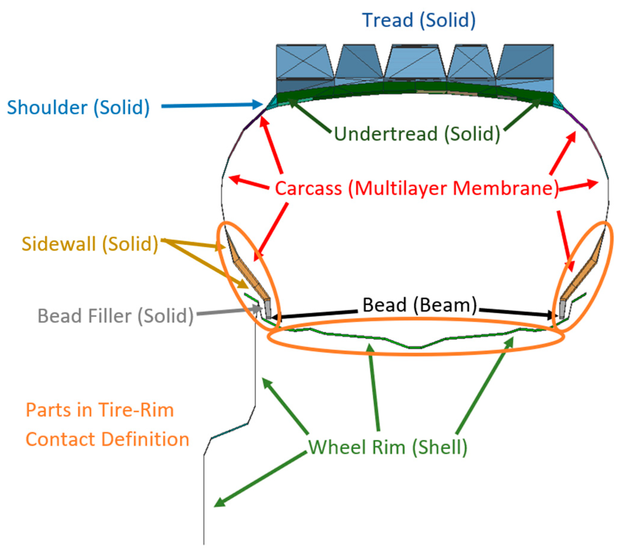
2.1. Tire Model

The FEA tire model used was modified from the Goodyear 315/80R22.5 RHD truck tire model created and validated by Slade [34]. Slade treated the tire–rim interface as a rigid body since the focus was on tire dynamics and determining rigid ring model parameters. The FEA tire model was composed of multiple types of elements, including shells, solids, beams, and multilayer membranes for the tire carcass [34]. The tire was then created by rotating the cross-section depicted in Figure 1 sixty times.

2.2. Contact Model

A new contact was defined at the tire–rim interface to mimic the tire–rim slip. The components of the tire–rim contact definition are depicted in Figure 1. On the tire side, there were two solid elements, the sidewall and bead filler, while on the rim side, the entire ledge part of the rim formed part of the contact to prevent the tire elements from passing through the solid rim. A symmetric node-to-segment type contact was computationally efficient and effective for the contact between solid and shell elements. The symmetry of the contact meant that nodes on each side of the contact were checked for penetration of the other side, reducing penetration compared to a one-way contact. Symmetric contacts like this have been used in existing research [25] and are recommended for crash analysis in LS-DYNA [45]. A contact thickness of 0.5 mm was found by trial and error to be the smallest thickness that still avoided penetration.

Additional contacts were also needed to define the interactions between the tire and the SPH soil, as well as the SPH soil and the box created to contain the soil (Figure 2). The soil box was defined as a rigid body made of null shell material and had a non-symmetric contact with the SPH soil, with a contact thickness of 2 mm and a friction coefficient of 0.6. The tire–soil contact included the entire tire and rim (except the hub) and had the same parameters as the soil–box contact, except that the contact thickness was increased to 5 mm. All of the contacts used a simple Coulomb friction model with a constant friction coefficient μ. This means that the peak tangential force transmitted through the contact was $\mu F_z$. This friction model was chosen due to its simplicity and ease of implementation, in contrast to realistic friction models, which are substantially more complex [23].

Realistic friction models take into consideration the microstructure of the contacting surfaces and the physical mechanisms by which forces are applied, and energy is transferred/dissipated between contacting molecular structures. Energy dissipation in rubber is viscoelastic; therefore, the effects of sliding speed, temperature, and normal load need to be considered [46]. Since the Coulomb friction model used in this study does not include these effects, the tire–rim contact forces at high tire–rim slip rates may be overestimated. Furthermore, heat generation during the slipping process is known to decrease the friction coefficient [47] and would thus increase the instantaneous rim slip. Predicting the exact effects would require a thermal-friction model, which is beyond the scope of this study but would be a possible avenue for future research.

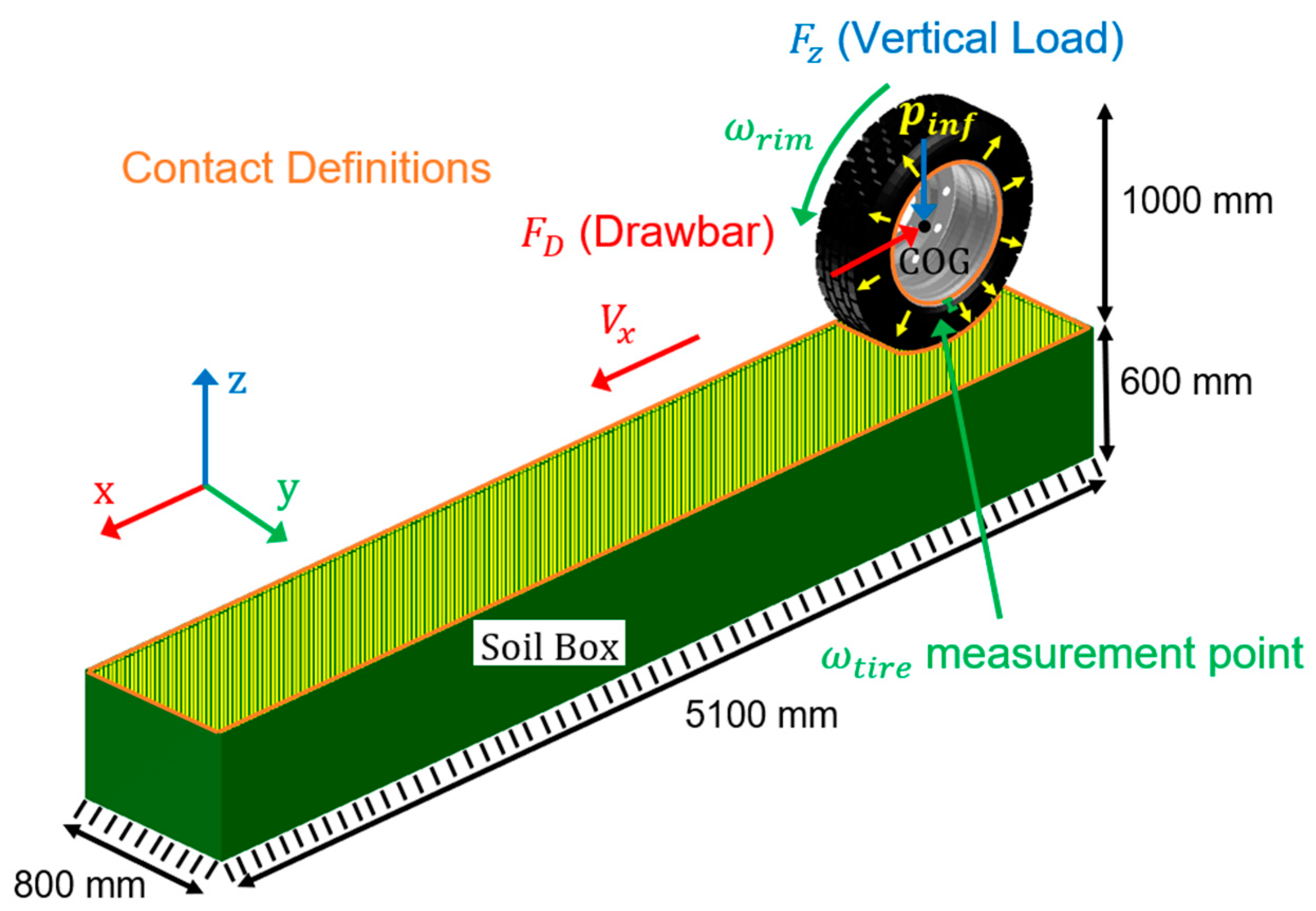
2.3. Boundary Conditions

To control the behaviour of the tire and soil models, a range of loads and constraints were applied; the most significant of these are displayed in Figure 2. Global constraints included gravity and an initial period of nodal damping to reduce oscillation in the results. Both the soil boxes and rims were treated as rigid bodies with a Center of Gravity (COG) node, and the soil boxes were fixed in place. The edge of the other three degrees of freedom for COGs was fixed, but they could rotate around the y-axis and translate in the x and z directions. Three loads were applied to the rim COG: a vertical load $F_z$, a horizontal drawbar load $F_x$, and a constant angular velocity ${\omega }_{rim}$. $F_z$ represented the weight of the vehicle resting on that tire, $F_x$ represented the towed weight used in a tire–rim slip test [1] and ${\omega }_{rim}$ was used to impose a specified longitudinal speed $V_x$ on the driven tire–rim combination. Additional loads were the constant surface pressure $p_{inf}$ applied to the inside of the tire carcass to represent the inflation pressure, and nodal damping applied to some of the carcass sidewall elements to simulate the viscous effects of the tire rubber. The magnitude of this sidewall damping depended on the inflation pressure and resulting vibration modal frequencies of the tire [48], but in this case, the sidewall damping had little effect due to the low speeds used for the soil simulations and the large damping effect of the soil itself.

The total simulation time was 1.5 s, with an initial time-step of 1 × 10⁻⁶ s, after which the time steps were determined adaptively by the solver. There are two reasons for this length of total simulation time. First, it helps the simulation run in a reasonable amount of real-time (approx. 12 h), considering the small time-step and large number of SPH particles to be simulated. Second, this amount of simulation time is sufficient for the tire model to reach steady-state and complete at least 3 revolutions for taking a good steady-state average of the results. All of the loads were fully applied within the first 0.4 s. The results were taken from the largest steady-state region between 0.5 and 1.5 s. Five different simulation parameters were then varied, as listed in

Table 1. Parameters varied for tire–rim slip simulations.

Parameter	Range	Default Value
$V_x$	5–60 km/h	10 km/h
$\mu$	0.1–0.9	0.2
$F_x$	20–90%	60%
$F_z$	13–41 kN	41 kN
$p_{inf}$	276–758 kPa	379 kPa

, to determine their independent effects on the tire–rim slip. In a given simulation run, four of the parameters were set to the default value, while the fifth took on a discrete value within the range in Table 1. The default values were purposely chosen to characterize a simulation where tire–rim slip was likely, with a high drawbar and vertical loads and a low inflation pressure and tire–rim friction coefficient. This was conducted in order to obtain results showing the transition region from rim-slip to no rim-slip. Also, the high loads reflect the parameters used in ASTM F2803 for physically qualifying the rim-slip performance of tires [1].

2.4. Tire–Rim Slip Measurement

Tire–rim slip was measured by a new quantity called rim-slip ($i_{rim}$), which was calculated from the angular velocities of the tire and rim (${\omega }_{tire}$ and ${\omega }_{rim}$) via Equations (1) and (2) [5]. Equation (1) was used to obtain the results presented here since a positive torque was applied to rotate the rim at a steady speed. ${\omega }_{rim}$ was an input to the simulation while ${\omega }_{tire}$ was measured using the COG of a small rigid body added to the sidewall (Figure 2).

$$\begin{array}{cc}\hfill \mathrm{accelerating}& i_{rim}=\left(1-\frac{{\omega }_{tire}}{{\omega }_{rim}}\right)\times 100\mathrm{\%}\end{array}$$

(1)

$$\begin{array}{cc}\hfill \mathrm{braking}& i_{rim}=\left(1-\frac{{\omega }_{rim}}{{\omega }_{tire}}\right)\times 100\mathrm{\%}\end{array}$$

(2)

In order to make the drawbar load behave like a real rolling-resistance-based load, which goes to zero when it stops moving, a sensor was included that switched off the drawbar load when the wheel COG’s velocity relative to the soil box dropped below 0.036 km/h. The inclusion of this sensor resulted in a simple control effect that ensured the wheel became virtually stationary once the tire slipped on the rim.

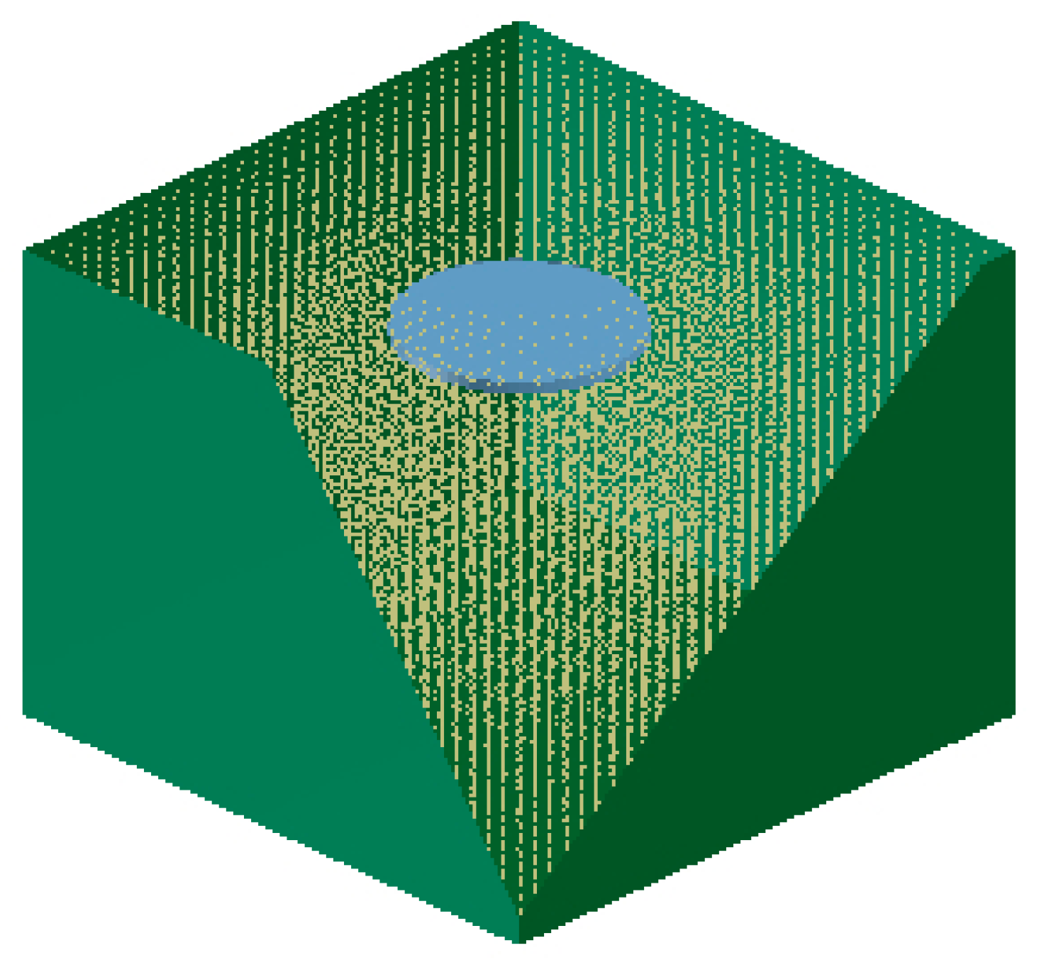
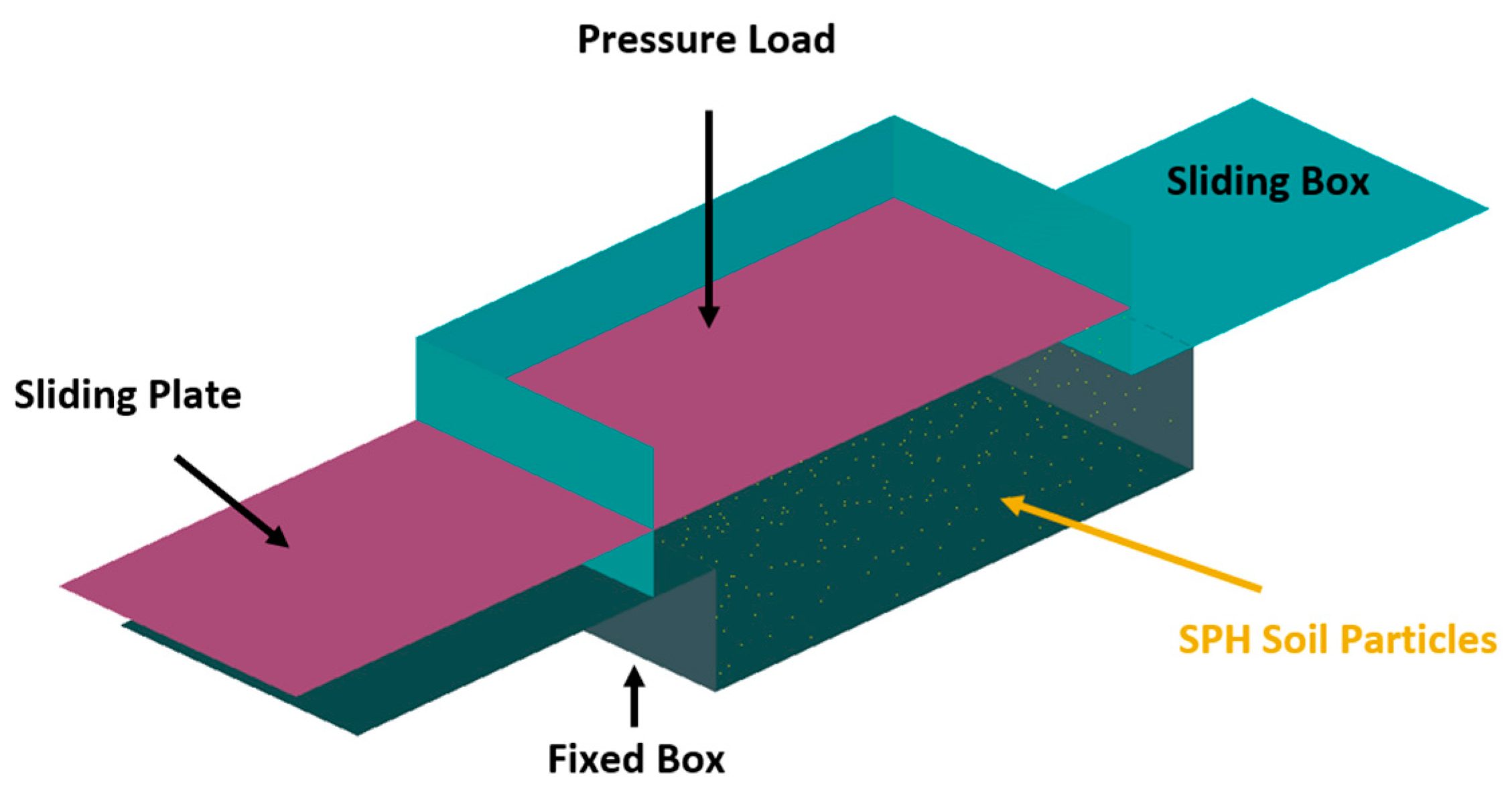
2.5. Soil Model and Calibration

The soil chosen for simulation was an upland sandy loam, characterized using the Bekker equation coefficients in

Table 2. Bekker equation coefficients obtained from upland sandy loam measurements [8].

Coefficient	Units	Value
$n$	none	1.10
$k_c$	kN/mn+1	74.6
$k_{\varphi }$	kN/mn+2	2080
$c$	kPa	3.3
$\varphi$	deg	33.7

reported by Wong [8]. These coefficients form Equations (3) and (4), which characterize the pressure-sinkage and shear stress behaviour of the soil:

$$p=(\frac{k_c}{b}+k_{\varphi })z^n$$

(3)

$${\tau }_{max}=c+p\tan \varphi$$

(4)

where $z$ is the vertical soil sinkage in m, $b$ is the contact patch size in m, $p$ is the normal pressure applied to the soil in kPa, ${\tau }_{max}$ is the maximum shear stress in kPa, and the other coefficients (see Table 2) are determined from empirical curve-fitting [8].

The soil was simulated in PAM-CRASH 2013 using SPH elements, whose parameters were calibrated following the method of El-Sayegh et al. [49]. In this calibration method, pressure-sinkage and direct-shear tests were simulated, as shown in Figure 3 and Figure 4. The soil was loaded at a range of pressures from 0 to 200 kPa, and then the maximum vertical sinkage and the maximum shear stress were extracted and plotted to form a set of curves describing the behaviour of the simulated soil. The simulated soil curves were then graphically and quantitatively (using R² and MSE metrics) compared with the curves generated by plotting Equations (1) and (2) through the same range of pressures. The parameters of the SPH soil model were varied through a series of trials until a trial with sufficient closeness to the measured curves was found. The final parameters used in the tire–rim slip simulations on the upland sandy loam were a density of 1.40 g/cm³, an elastic modulus of 0.27 MPa, a yield strength of 0.012 Mpa, a shear modulus of 6.0 Mpa, and a bulk modulus of 25 Mpa.

3. Results

This section describes the independent effects of the five varied parameters on the amount of tire–rim slip on the upland sandy loam soil. Comparisons are also made with a hard surface in order to determine the terrain on which tire–rim slip is more likely to occur.

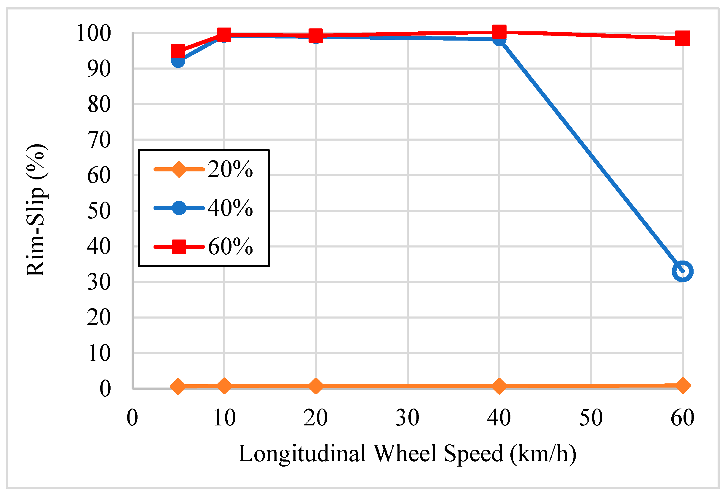
3.1. Effect of Longitudinal Wheel Speed

The wheel’s longitudinal speed was the first parameter whose impact on tire–rim slip was examined. Figure 5 illustrates how little the longitudinal wheel speed affected the percent rim-slip, which remained nearly constant at all speeds. This effect was repeated for each of the different drawbar loads, with the exception of one outlier under the 40% drawbar load, 60 km/h condition. Both the 40% and the 60% drawbar loads caused 100% rim slip to occur, and presumably, a higher drawbar load of 90% would also cause 100% rim slip on the soil. Therefore, in the interest of acquiring greater information, the third speed-variation simulation was run with a lower drawbar load of 20% (orange line), which showed 0% rim slip. Thus, it can be concluded that the transition from 0% to 100% rim-slip occurs at lower drawbar loads between 20% and 40%.

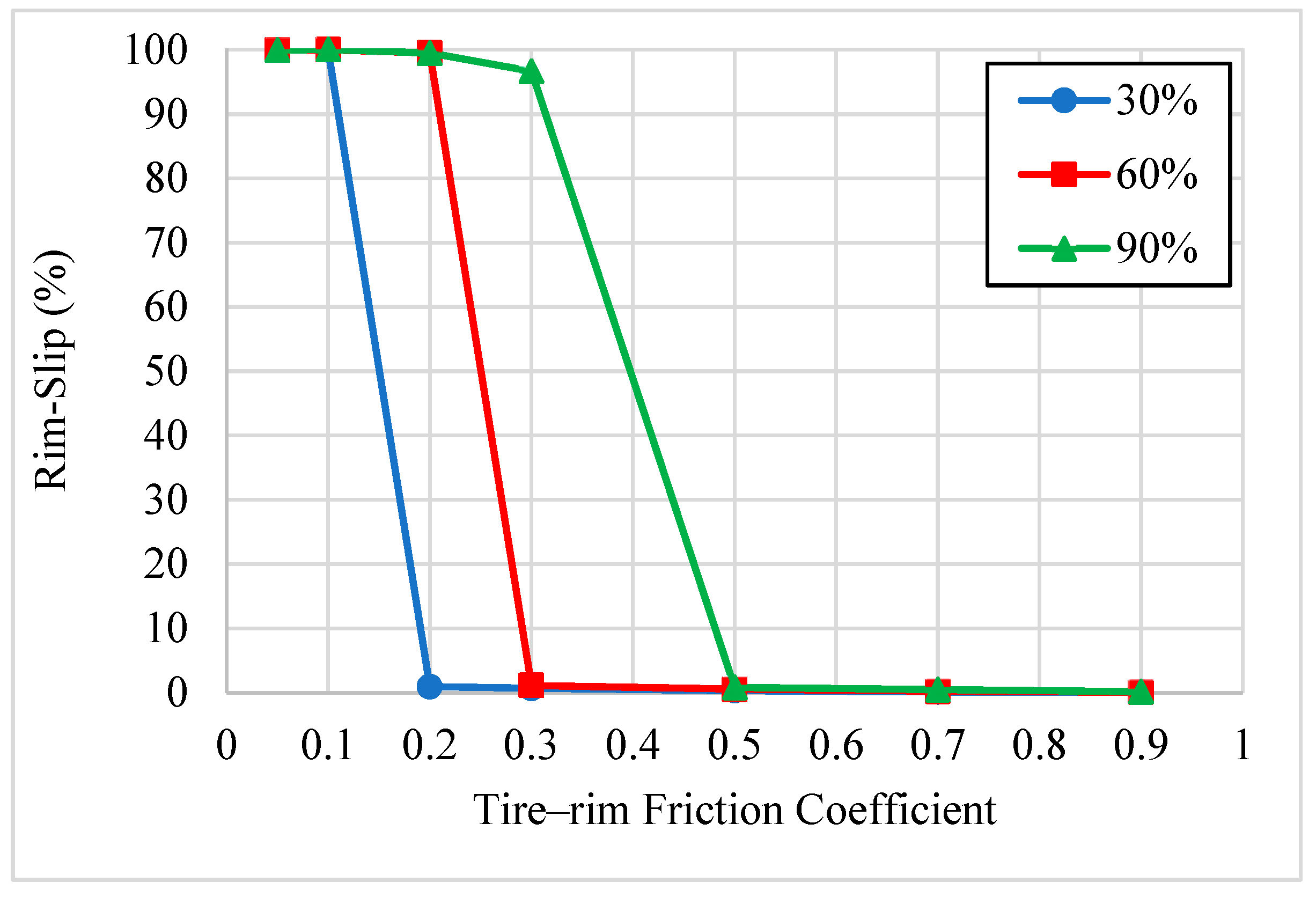
3.2. Effect of Friction Coefficient and Drawbar Load

The effect on the tire–rim slip of changing the tire–rim friction coefficient and drawbar load is shown in Figure 6. A lower tire–rim friction coefficient generally resulted in a larger rim-slip, while a lower drawbar load caused less rim-slip. A threshold effect was noticeable where the rim slip changed from about 0% to about 100% after a particular combination of friction coefficient and drawbar load was reached, the same as found in previous research [5]. It is notable that the tire–rim friction coefficient needed to decrease to at least 0.3 in order for a large amount of tire–rim slip to occur, even for a high drawbar load of 90%.

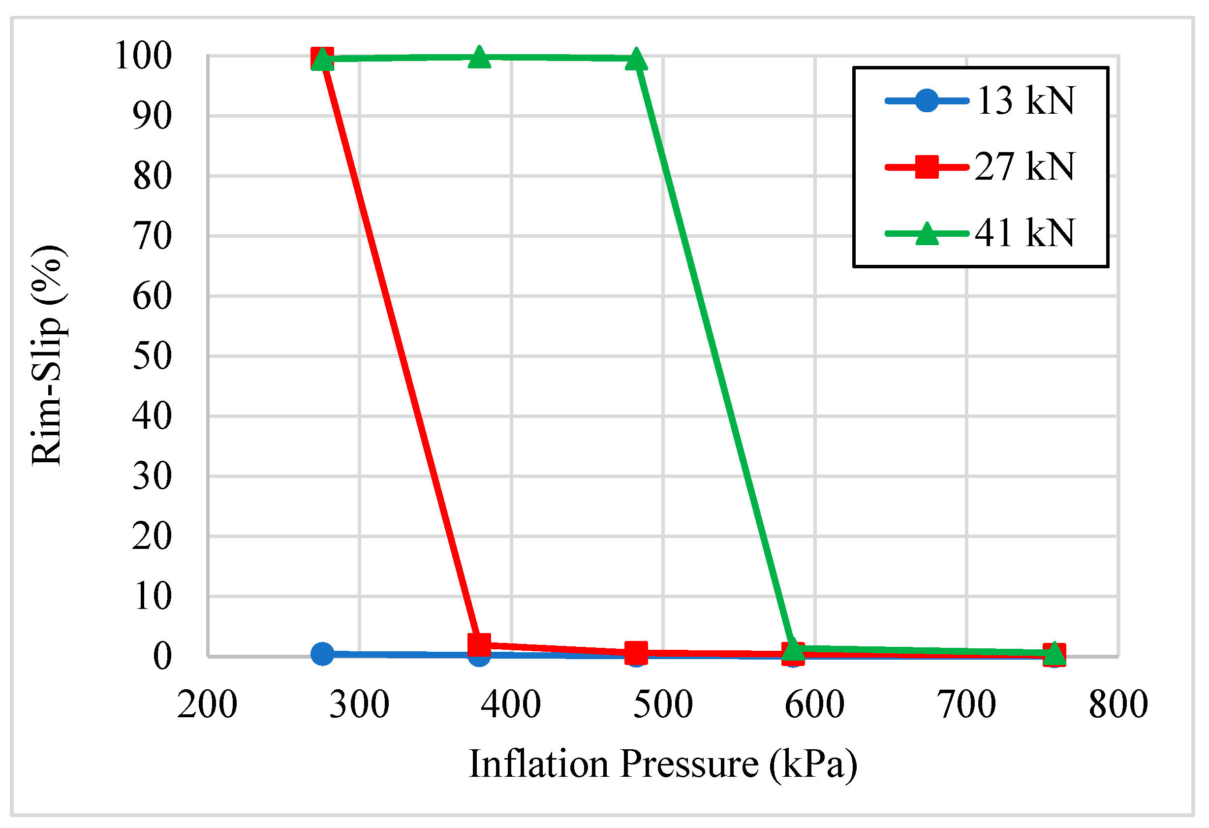
3.3. Effect of Vertical Load and Inflation Pressure

The last two parameters investigated were the vertical load and the inflation pressure. As seen in Figure 7, tire–rim slip on soil occurred with a 41 kN vertical load up to an inflation pressure of 482 kPa, while the lighter 27 kN vertical load only slipped below 379 kPa, and the 13 kN vertical load did not have tire–rim slip at any tested pressure. The fact that tire–rim slip only occurred well below the rated 896 kPa inflation pressure of the tire indicated that tire–rim slip is a low-pressure phenomenon on the soil. Increasing the vertical load also substantially increases the amount of tire–rim slip experienced.

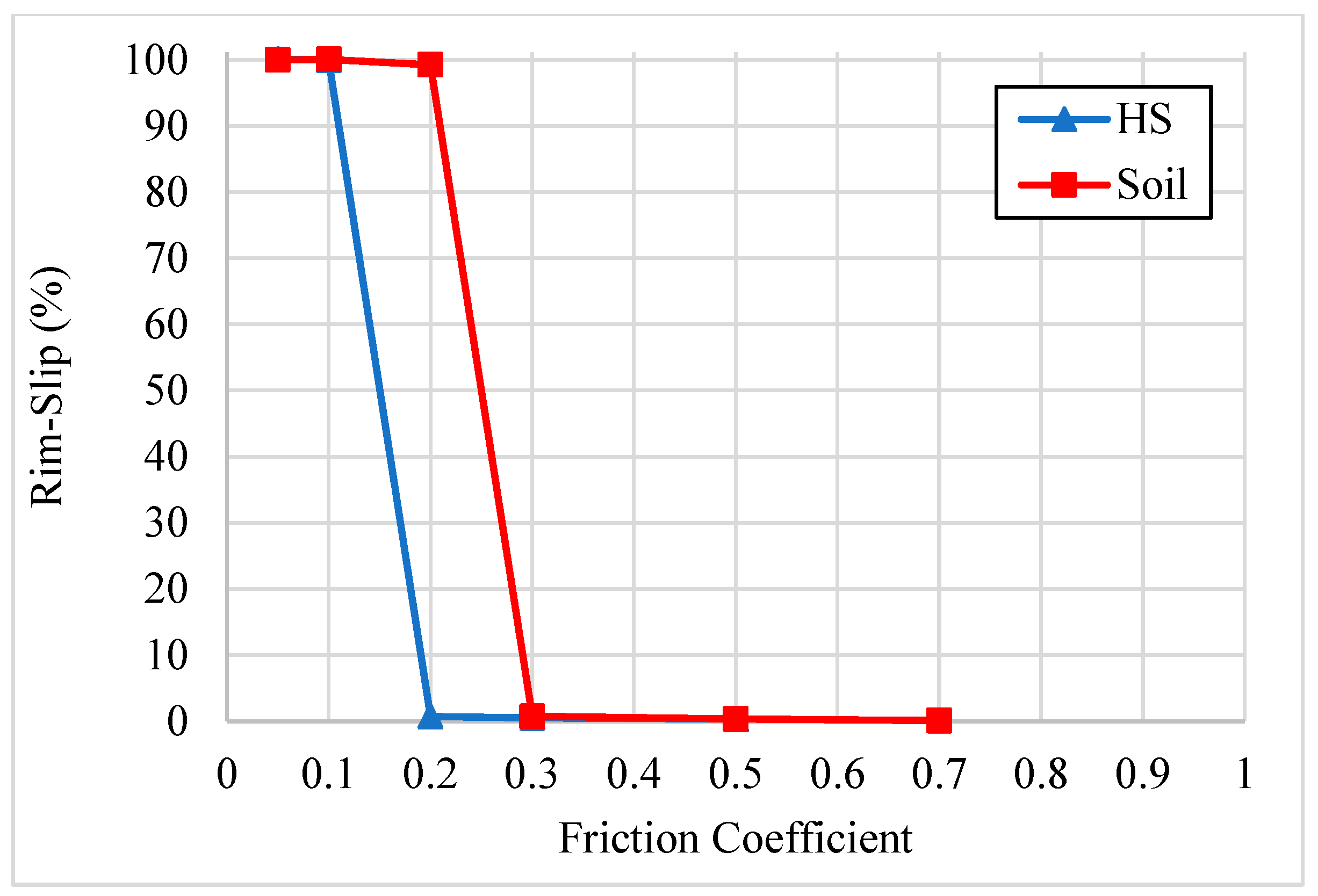
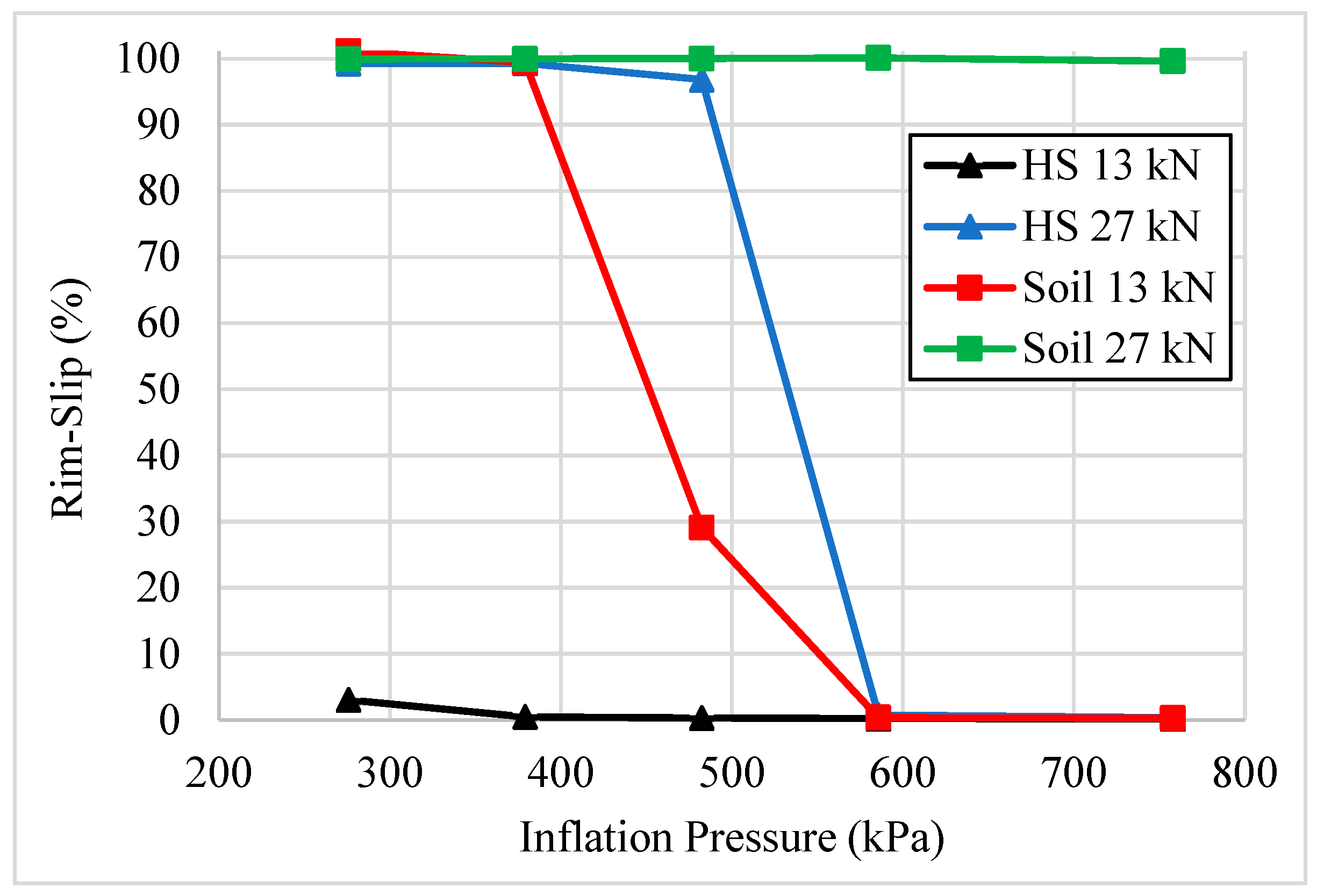
3.4. Comparison with Hard Surface

Results in this section are presented by comparing the tire–rim slip on soil and on a hard surface at various combinations of parameters. The combinations are different than in the previous sections, and the continued presence of the threshold effect indicates its widespread nature. In Figure 8, both the soil and hard surface have a similar trend where there is a low threshold value for the friction coefficient, beyond which the rim slip drops to zero. However, there is a noticeable difference in that the soil had a rim-slip of 99.2% at 0.2 friction, whereas the hard surface had a rim-slip of 0.7% at 0.2 friction. This means that the entire curve was shifted to the right for the soil. Thus, it can be concluded that the soil had more rim-slip than the hard surface near the threshold friction coefficient value when all of the other parameters are the same.

It is also instructive to compare the rim-slip on soil and a hard surface at different vertical loads, as is shown in Figure 9. At 13 kN, the hard surface has essentially 0% rim-slip, while on the soil, the rim-slip increases to 29% at 482 kPa and 99.4% at 379 kPa. In addition, while at 27 kN, the hard surface does have non-zero rim-slip at 482 kPa and below, at 27 kN, the soil has 100% rim-slip at all of the tested inflation pressures. The large amount of rim-slip is due to the very low friction coefficient of 0.05 used, but since the hard surface had the same low tire–rim friction coefficient, the soil is clearly more likely to have rim-slip at a given combination of parameters. Comparing the rim slip on soil and a hard surface at different drawbar loads generated similar results to Figure 9, adding to the conclusion that tire–rim slip is more likely on soil.

4. Conclusions

This study of tire–rim slip for a simulated RHD truck tire on upland sandy loam demonstrated the effects of different operating parameters as well as terrain type on tire–rim slip. The main results were:

• A threshold effect was visible for rim-slip.
• Increased drawbar and vertical loads caused increased rim-slip, increased friction coefficient, and inflation pressure decreased rim-slip, and longitudinal wheel speed had a negligible effect on rim-slip.
• A particular longitudinal wheel speed and drawbar load combination resulted in an outlier simulation with unsteady results.
• Compared to the hard surface, rim-slip occurred on the soil at lower vertical loads, higher friction coefficients, and higher inflation pressures.

The last point implies that tire–rim slip is more likely to occur on soil than on a hard surface; therefore, it is an issue worth considering when designing tire and wheel systems for off-road operations. These conclusions about the amount of tire–rim slip on soil apply only to the calibrated upland sandy loam. Other similar soils, such as a dry sandy loam, may have similar results, but the properties of soil vary widely, and further research is required to draw any general conclusions about the tire–rim slip effects of soil relative to a hard surface.

References

1. ASTM F2803-21; Standard Test Method for Evaluating Rim Slip Performance of Tires and Wheels. ASTM International: West Conshohocken, PA, USA, 2021. [CrossRef]
2. Bishel, S. Land Vehicle Tire Qualification, AD1086645, U.S.; Army DEVCOM Ground Vehicle Systems Center: Warren, MI, USA, 2019; Available online: https://apps.dtic.mil/sti/pdfs/AD1086645.pdf (accessed on 10 February 2024).
3. General Motors. Vibration Shortly After Tires are Mounted/Preventing Vibration from Wheel Slip (Tire Sliding on Wheel), 12-03-10-001B. 2014. Available online: https://static.nhtsa.gov/odi/tsbs/2014/MC-10137841-9999.pdf (accessed on 23 April 2021).
4. Nitto Tire. Consumer Complaints for Vibration—Tire/Rim Slip, NTSD-12-015. 2014. Available online: https://www.nittotire.com/media/55ibthri/techbulletin_ntsd_12-015-rev-3.pdf (accessed on 29 April 2021).
5. Collings, W.; El-Sayegh, Z.; Ren, J.; El-Gindy, M. Modelling of Off-Road Truck Tire-Rim Slip Using Finite Element Analysis. SAE Int. J. Adv. Curr. Pract. Mobil. 2022, 4, 2335–2341. [Google Scholar] [CrossRef]
6. Pacejka, H. Tyre and Vehicle Dynamics, 1st ed.; Butterworth-Heinemann: Oxford, UK, 2002. [Google Scholar]
7. Pacejka, H. Analysis of the Dynamic Response of a Rolling String-Type Tire Model to Lateral Wheel-Plane Vibrations. Veh. Syst. Dyn. 1972, 1, 37–66. [Google Scholar] [CrossRef]
8. Wong, J. Theory of Ground Vehicles, 3rd ed.; John Wiley and Sons: New York, NY, USA, 2001. [Google Scholar]
9. Johnson, A.R.; Tanner, J.A.; Mason, A.J. A kinematically driven anisotropic viscoelastic constitutive model applied to tires. In Proceedings of the Workshop on Computational Modelling of Tires, Hampton, VA, USA, 26–27 October 1994; pp. 41–51. [Google Scholar]
10. Reida, J.D.; Boesch, D.A.; Bielenberg, R.W. Detailed tire modeling for crash applications. Int. J. Crashworthiness 2007, 12, 521–529. [Google Scholar] [CrossRef]
11. Barbani, D.; Pierini, M.; Baldanzini, N. FE modelling of a motorcycle tyre for full-scale crash simulations. Int. J. Crashworthiness 2012, 17, 309–318. [Google Scholar] [CrossRef]
12. Orengo, F.; Ray, M.H.; Plaxico, C.A. Modeling tire blow-out in roadside hardware simulations using LS-DYNA. In Proceedings of the ASME 2003 International Mechanical Engineering Congress and Exposition, Transportation: Making Tracks for Tomorrow’s Transportation, Washington, DC, USA, 15–21 November 2003; pp. 71–80. [Google Scholar]
13. Ballo, F.; Previati, G.; Gobbi, M.; Mastinu, G. Tire-rim interaction, a semi-analytical tire model. ASME. J. Mech. Des. 2018, 140, 041401. [Google Scholar] [CrossRef]
14. Hu, X.; Liu, X.; Shan, Y.; He, T. Simulation and Experimental Validation of Sound Field in a Rotating Tire Cavity Arising from Acoustic Cavity Resonance. Appl. Sci. 2021, 11, 1121. [Google Scholar] [CrossRef]
15. Hyttinen, J.; Österlöf, R.; Drugge, L.; Jerrelind, J. Constitutive rubber model suitable for rolling resistance simulations of truck tyres. Proc. Inst. Mech. Eng. Part D J. Automob. Eng. 2023, 237, 174–192. [Google Scholar] [CrossRef]
16. Anghelache, G.; Moisescu, R. Analysis of Rubber Elastic Behaviour and Its Influence on Modal Properties. Mater. Plast. 2008, 45, 143–148. [Google Scholar]
17. Pomoni, M. Exploring Smart Tires as a Tool to Assist Safe Driving and Monitor Tire–Road Friction. Vehicles 2022, 4, 744–765. [Google Scholar] [CrossRef]
18. Wang, Y.; Hu, J.; Wang, F.; Dong, H.; Yan, Y.; Ren, Y.; Zhou, C.; Yin, G. Tire Road Friction Coefficient Estimation: Review and Research Perspectives. Chin. J. Mech. Eng. 2022, 35, 6. [Google Scholar] [CrossRef]
19. Venturini, S.; Bonisoli, E.; Rosso, C.; Velardocchia, M. A tyre-rim interaction digital twin for biaxial loading conditions. Mech. Mach. Theory 2024, 191, 105491. [Google Scholar] [CrossRef]
20. Gheshlaghi, F. Modeling and Analysis of Off-Road Tire Cornering Characteristics. Master’s Thesis, Ontario Tech University, Oshawa, ON, Canada, 2022. [Google Scholar]
21. Lee, C. Rim Slip and Bead Fitment of Tires: Analysis and Design. Tire Sci. Technol. 2006, 34, 38–63. [Google Scholar] [CrossRef]
22. Pelle, R. FEM Simulation of the Tire/Rim Seating Process. Tire Sci. Technol. 1994, 22, 76–98. [Google Scholar] [CrossRef]
23. Reina, S. A Study of Layered Contact Problems with Particular Application to Tyre-Wheel Interfaces. Ph.D. Dissertation, Imperial College, London, UK, 2010. [Google Scholar]
24. Cosseron, K.; Mellé, D.; Hild, F.; Roux, S. Optimal parameterization of tire-rim interaction for aircraft wheeSls. J. Aircr. 2019, 56, 2032–2046. [Google Scholar] [CrossRef]
25. Cai, Y.; Zang, M.; Duan, E. Modeling and Simulation of Vehicle Responses to Tire Blowout. Tire Sci. Technol. 2015, 43, 242–258. [Google Scholar] [CrossRef]
26. ESI Group. Virtual Performance Solution 2014: Solver Reference Manual; ESI Group: Rungis, France, 2014. [Google Scholar]
27. Wriggers, P. Computational Contact Mechanics, 2nd ed.; Springer: Berlin, Germany, 2006; ISBN 978-3-540-32609-0. [Google Scholar]
28. Herron, J.R. Application of ALE Contact to Composite Shell Finite Element Model for Pneumatic Tires. Master’s Thesis, University of Toledo, Toledo, OH, USA, 2005. [Google Scholar]
29. Previati, G.; Ballo, F.; Gobbi, M.; Mastinu, G. Radial impact test of aluminium wheels—Numerical simulation and experimental validation. Int. J. Impact Eng. 2019, 126, 117–134. [Google Scholar] [CrossRef]
30. Ge, H.; Quezada, J.C.; Le Houerou, V.; Chazallon, C. Multiscale analysis of tire and asphalt pavement interaction via coupling FEM–DEM simulation. Eng. Struct. 2022, 256, 113925. [Google Scholar] [CrossRef]
31. Bekker, M.G. Land Locomotion Research Report No. 5; Detroit Arsenal: Warren, MI, USA, 1958. [Google Scholar]
32. Reece, A.R. Problems of Soil Vehicle Mechanics; Rep. no. 8470, U.S.; Army Tank-Automotive Center: Warren, MI, USA, 1964; Available online: https://apps.dtic.mil/sti/citations/AD0450151 (accessed on 16 January 2021).
33. Smith, W.; Melanz, D.; Senatore, C.; Iagnemma, K.; Peng, H. Comparison of discrete element method and traditional modeling methods for steady-state wheel-terrain interaction of small vehicles. J. Terramech. 2014, 56, 61–75. [Google Scholar] [CrossRef]
34. Slade, J.L. Development of a New Off-Road Rigid Ring Model for Truck Tires Using Finite Element Analysis Techniques. Master’s Thesis, Pennsylvania State University, State College, PA, USA, 2009. [Google Scholar]
35. Ranvir, D.S. Development of Truck Tire Terrain Finite Element Analysis Models. Master’s Thesis, Ontario Tech University, Oshawa, ON, Canada, 2013. [Google Scholar]
36. Shokouhfar, S. A Virtual Test Platform for Analyses of Rolling Tyres on Rigid and Deformable Terrains. Ph.D. Dissertation, Concordia University, Montreal, QC, Canada, 2017. [Google Scholar]
37. Swamy, V.S.; Pandit, R.; Yerro, A.; Sandu, C.; Rizzo, D.M.; Sebeck, K.; Gorsich, D. Review of modeling and validation techniques for tire-deformable soil interactions. J. Terramechanics 2023, 109, 73–92. [Google Scholar] [CrossRef]
38. Cundall, P.; Strack, O. A discrete numerical model for granular assemblies. Géotechnique 1979, 29, 47–65. [Google Scholar] [CrossRef]
39. Gorsich, D.; Letherwood, M.; Dasch, J. Predicting mobility in military operational scenarios. Truck. Off-Highw. Eng. 2022, 30, 14–18. [Google Scholar]
40. Gingold, R.A.; Monaghan, J.J. Smoothed particle hydrodynamics: Theory and application to non-spherical stars. Mon. Not. R. Astr. Soc. 1977, 181, 275–389. [Google Scholar] [CrossRef]
41. Bagheri, M.; Mohammadi, M.; Riazi, M. A review of smoothed particle hydrodynamics. Comp. Part. Mech. 2023. [Google Scholar] [CrossRef]
42. Tasora, A.; Mangoni, D.; Negrut, D.; Serban, R.; Jayakumar, P. Deformable soil with adaptive level of detail for tracked and wheeled vehicles. Int. J. Veh. Perform. 2019, 5, 60–76. [Google Scholar] [CrossRef]
43. El-Sayegh, Z. Modelling and Analysis of Truck Tire-Terrain Interaction. Ph.D. Dissertation, Ontario Tech University, Oshawa, ON, Canada, 2020. [Google Scholar]
44. Huang, W.; Wong, J.Y.; Preston-Thomas, J.; Jayakumar, P. Predicting terrain parameters for physics-based vehicle mobility models from cone index data. J. Terramechanics 2020, 88, 29–40. [Google Scholar] [CrossRef]
45. DYNAmore GmbH. LS-DYNA Support: Contact Types. Available online: https://www.dynasupport.com/tutorial/contact-modeling-in-ls-dyna/contact-types (accessed on 9 February 2024).
46. Heinrich, G.; Klüppel, M. Rubber friction, tread deformation and tire traction. Wear 2008, 265, 1052–1060. [Google Scholar] [CrossRef]
47. Persson, B.N.J. Rubber friction: Role of the flash temperature. J. Phys. Condens. Matter 2006, 18, 7789. [Google Scholar] [CrossRef]
48. Chae, S. Nonlinear Finite Element Modeling and Analysis of a Truck Tire. Ph.D. Dissertation, Pennsylvania State University, State College, PA, USA, 2006. [Google Scholar]
49. El-Sayegh, Z.; El-Gindy, M.; Johansson, I.; Öijer, F. Off-road soft terrain modelling using smoothed particle hydrodynamics technique. In Proceedings of the ASME 2018 International Design Engineering Technical Conferences & Computers and Information in Engineering Conference, Quebec City, QC, Canada, 26–29 August 2018. [Google Scholar]
Figure 1. Tire–rim contact definition, various components, and cross-section of the FEA tire model (adapted from [5]).
Geotechnics 04 00012 g001
Figure 2. Loads, constraints, and contacts applied to tire–rim slip simulation on soil. The soil box length corresponds to the longitudinal wheel speed, in this case, 10 km/h.
Geotechnics 04 00012 g002
Figure 3. Cross-section of simulation setup for pressure-sinkage test. Pressure loads are applied to a 150 mm-radius rigid disk (blue) located in a rigid box (green) containing SPH particles (yellow). One corner of the box has been sectioned to improve the visibility of the SPH particles.
Geotechnics 04 00012 g003
Figure 4. Section through which the direct-shear test simulation is set up.
Geotechnics 04 00012 g004
Figure 5. Impact of drawbar load and longitudinal wheel speed on tire–rim slip on soil for a tire running at 379 kPa inflation pressure, 0.2 tire–rim friction coefficient, and 41 kN vertical load.
Geotechnics 04 00012 g005
Figure 6. Impact of drawbar load and tire–rim friction coefficient on tire–rim slip for soil. The other parameter settings were 379 kPa inflation pressure, 10 km/h longitudinal wheel speed, and 41 kN vertical load.
Geotechnics 04 00012 g006
Figure 7. Impact of vertical load and inflation pressure on the tire–rim slip for soil. The other parameter settings were 60% drawbar load, 0.2 tire–rim friction coefficient, and 10 km/h longitudinal wheel speed.
Geotechnics 04 00012 g007
Figure 8. Impact of friction coefficient on tire–rim slip for soil and hard surface (HS). The other parameter settings were 40% drawbar load, 379 kPa inflation pressure, 10 km/h longitudinal wheel speed, and 41 kN vertical load.
Geotechnics 04 00012 g008
Figure 9. Impact of inflation pressure on the tire–rim slip for soil and hard surface (HS). The other parameter settings were 30% drawbar load, 10 km/h longitudinal wheel speed, and 0.05 friction coefficient.
Geotechnics 04 00012 g009