
Stress–Strain–Time Description and Analysis of Frozen–Thawed Silty Clay under Low Stress Level

Abstract
:1. Introduction
2. Materials and Experimental Methods
2.1. Source of the Soil
2.2. Parameters of the Specimens
2.3. Test Conditions and Procedure
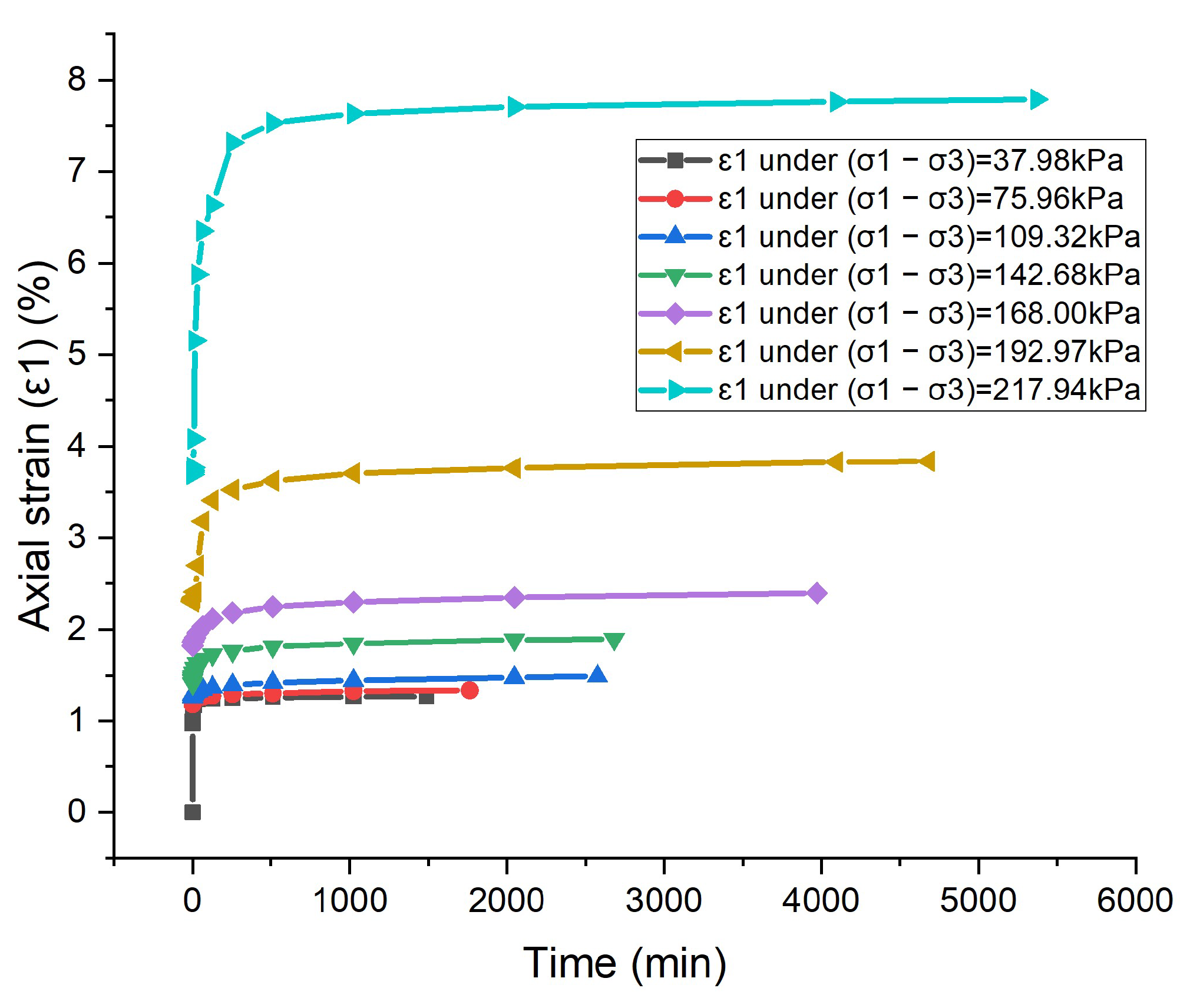
3. Results
4. Analysis
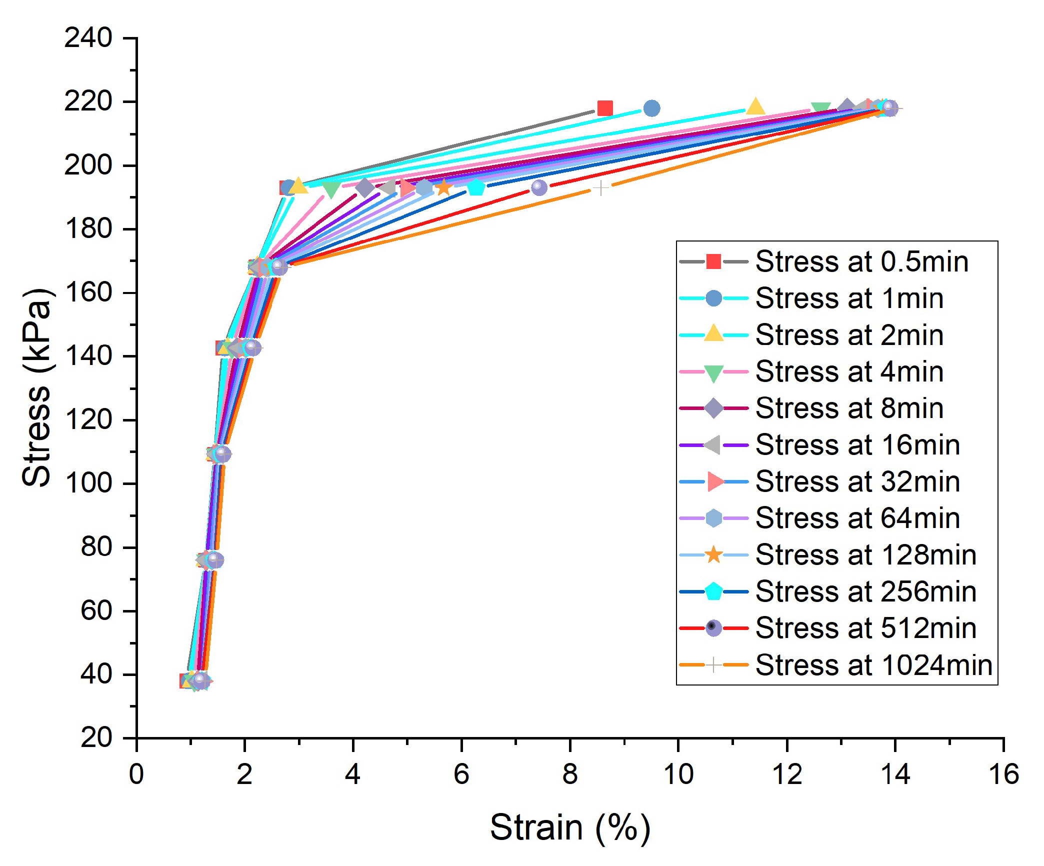
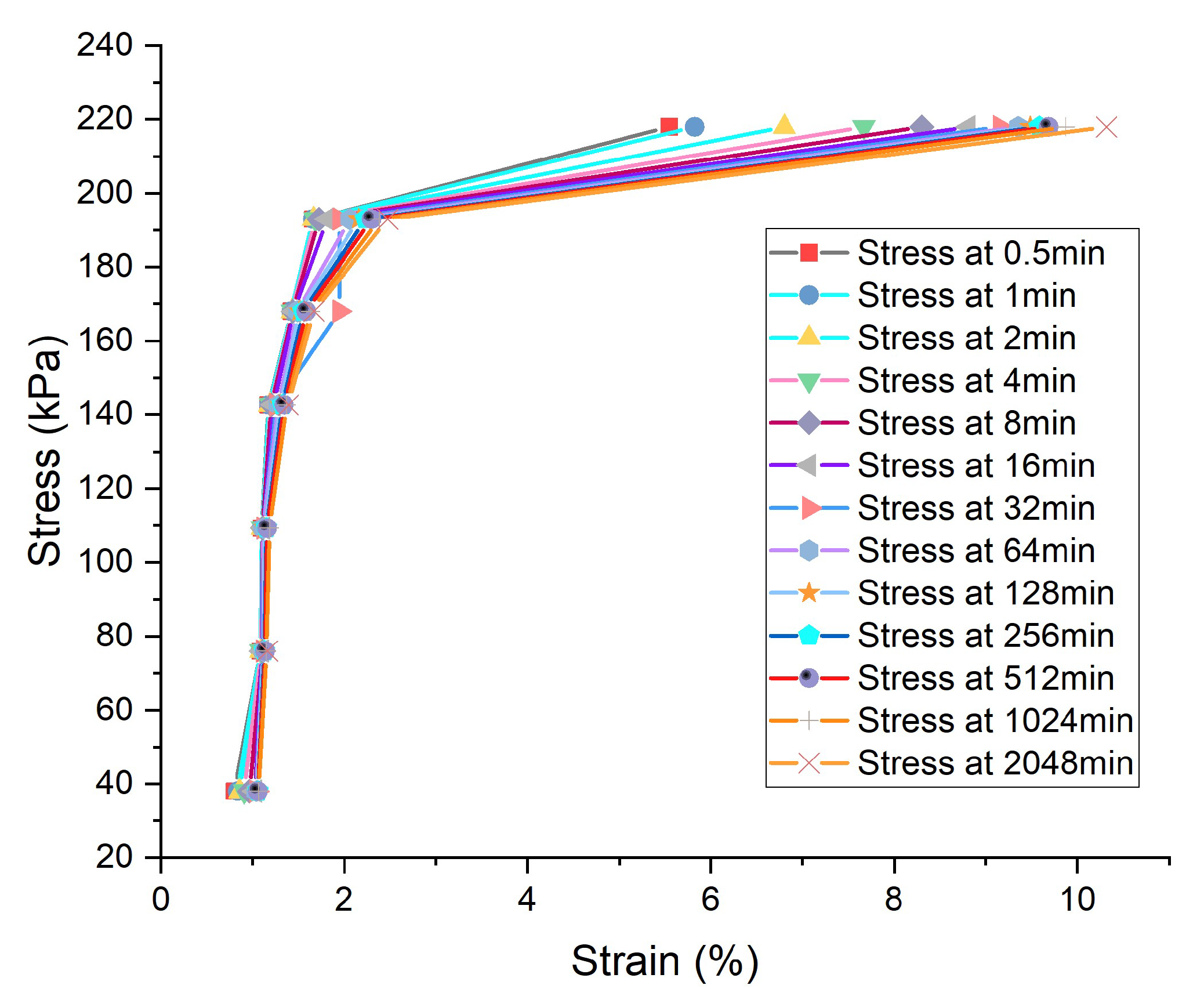
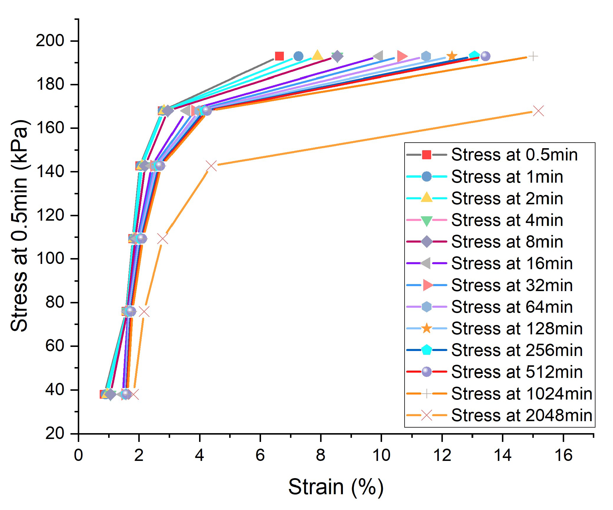
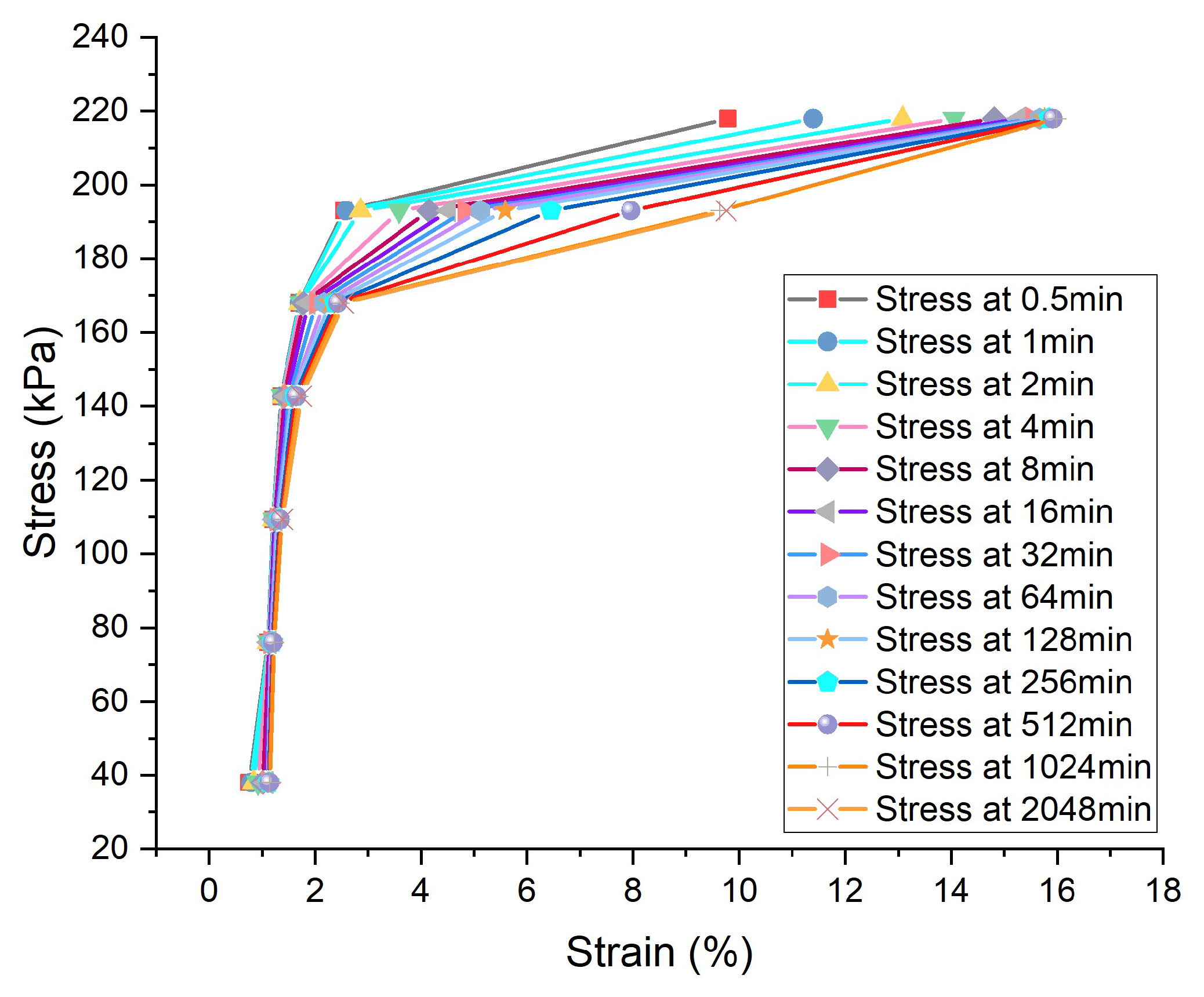
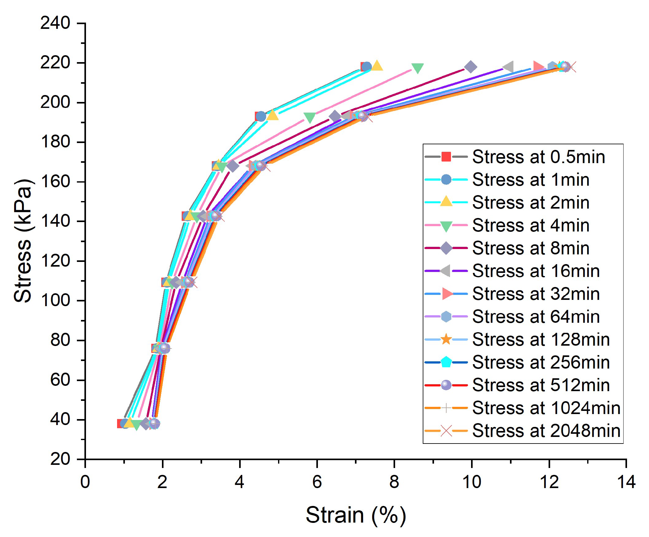
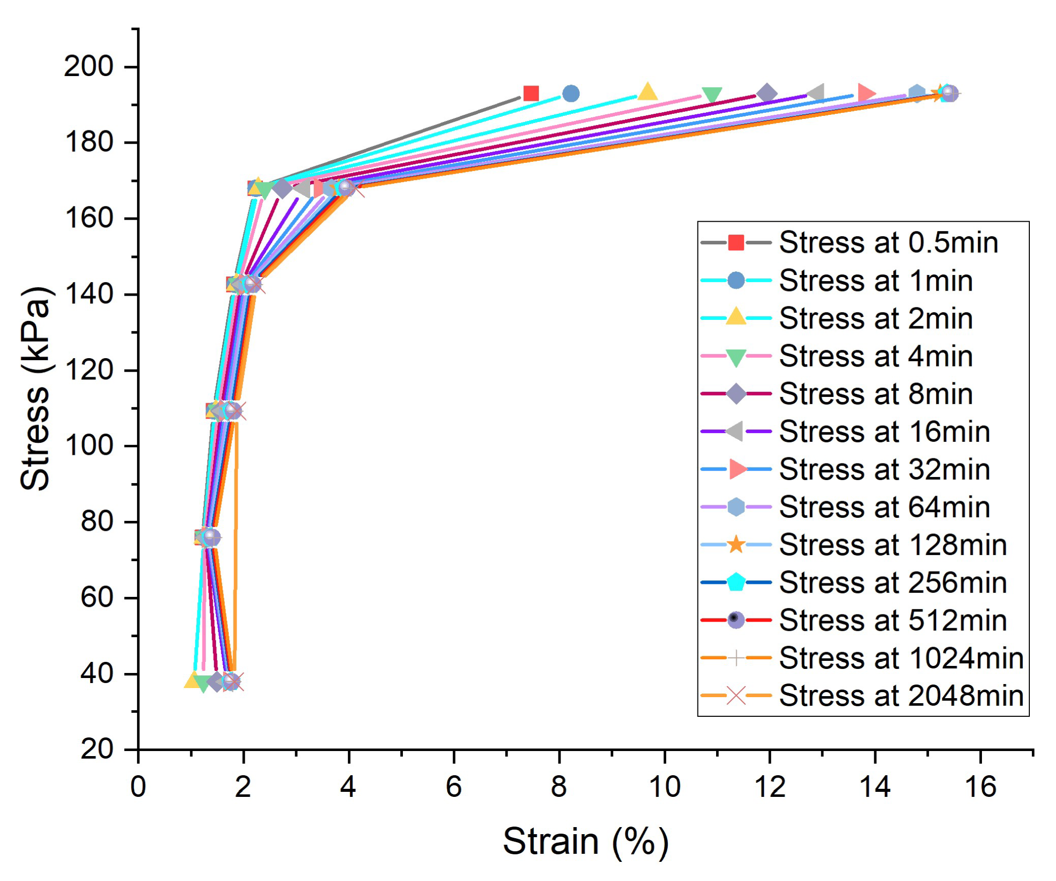
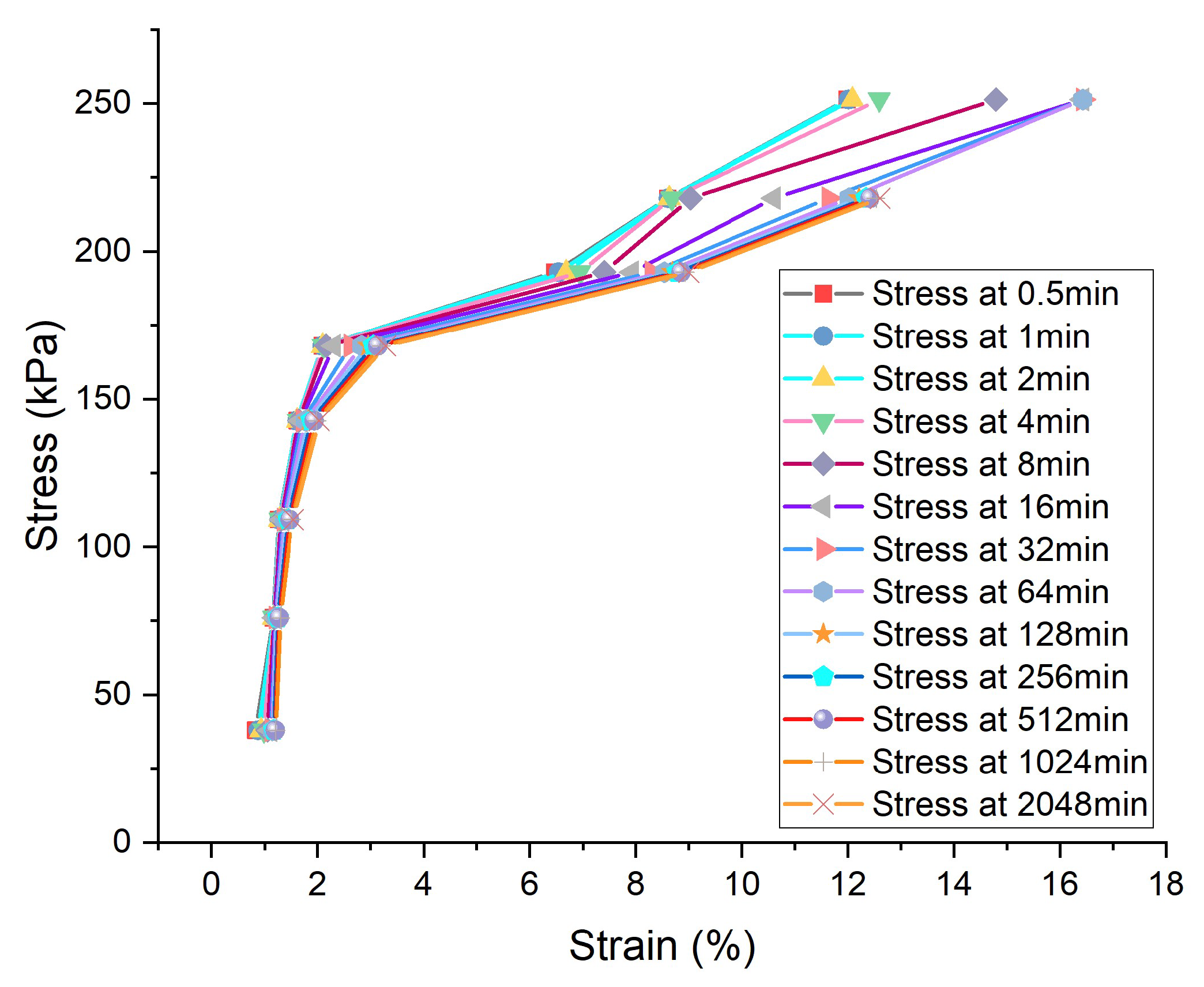
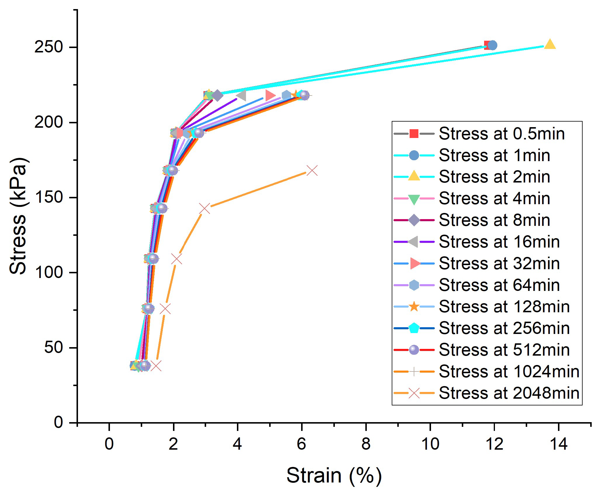
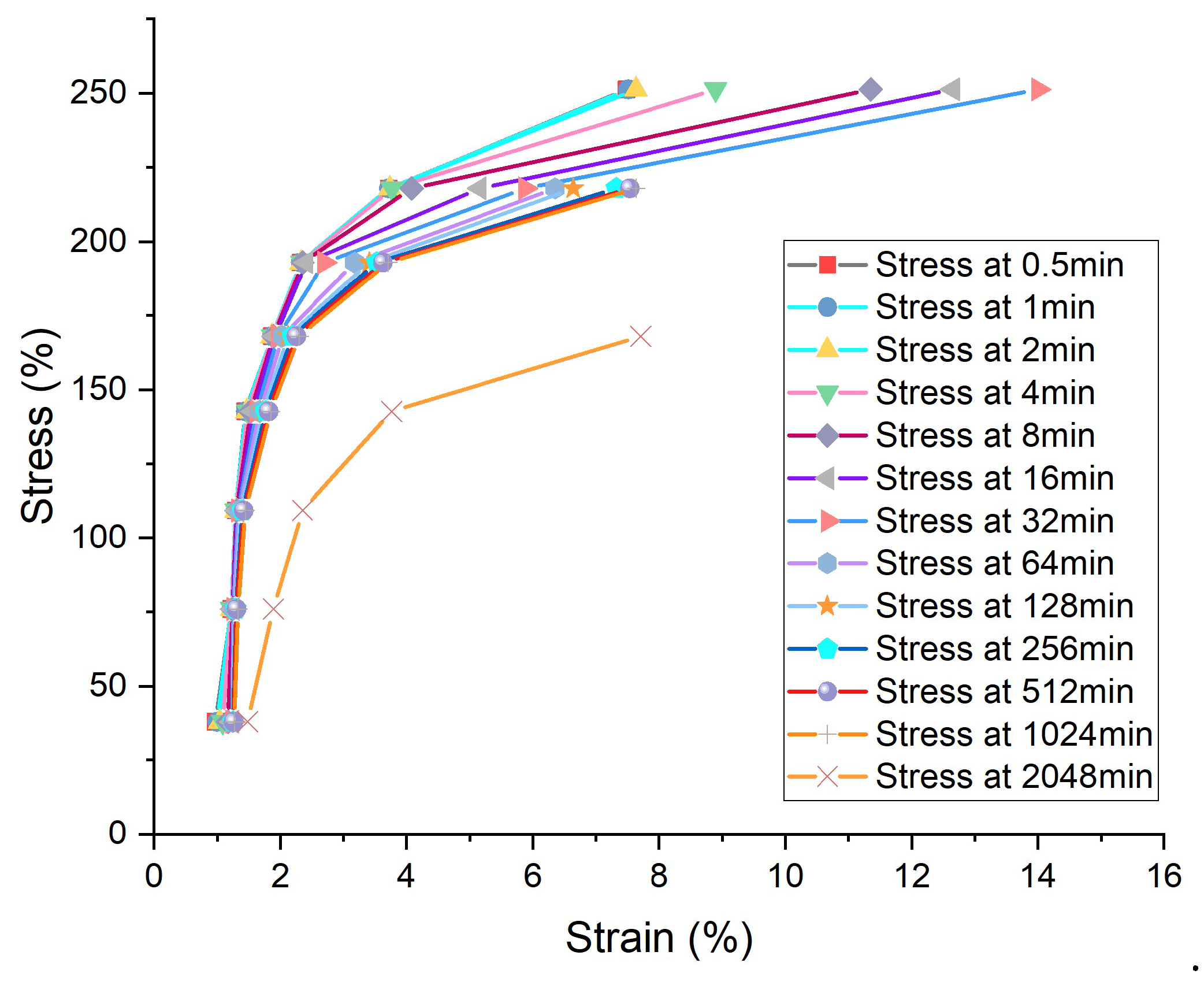
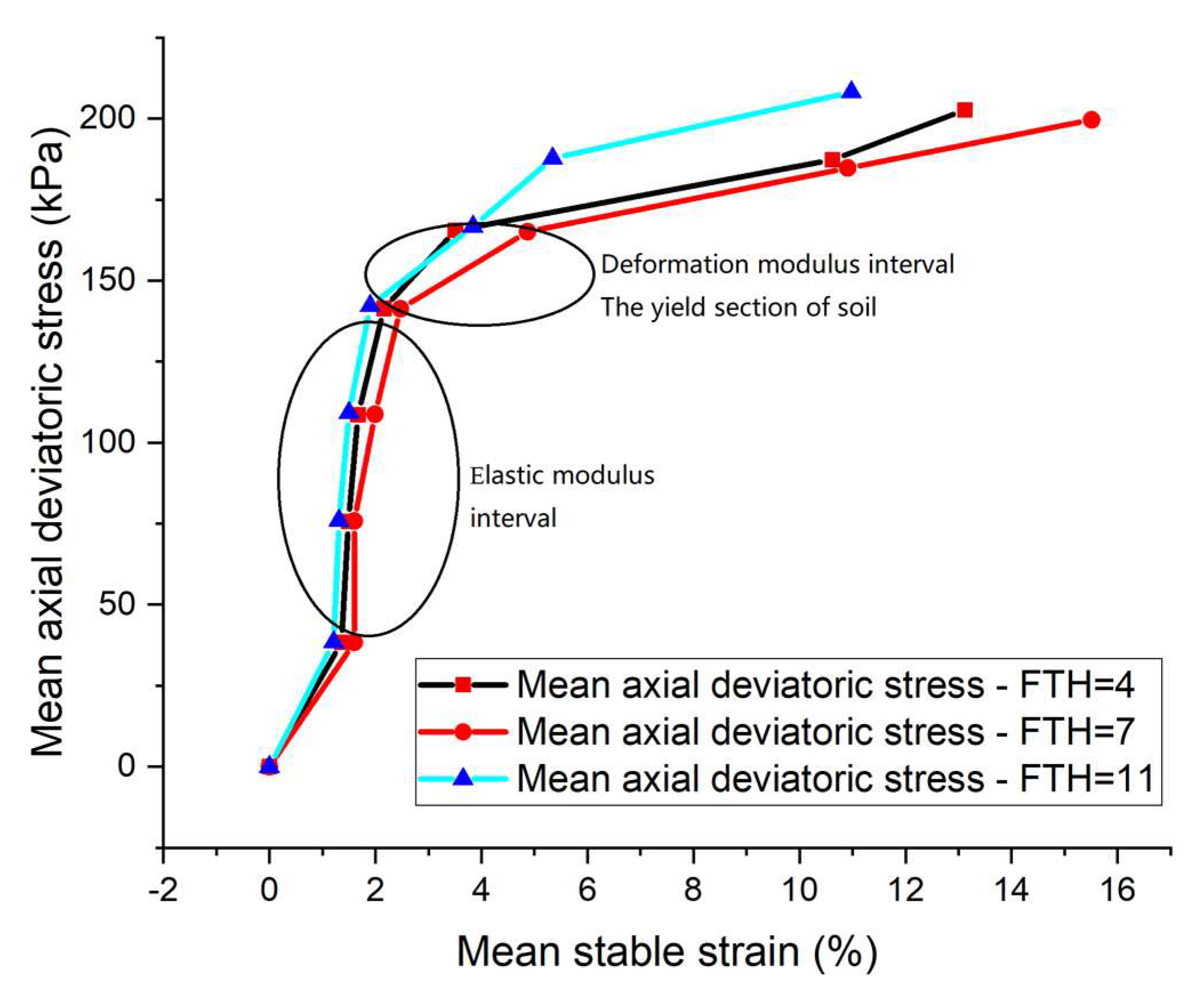
4.1. Analysis of the Isochronous Stress–Strain Curves
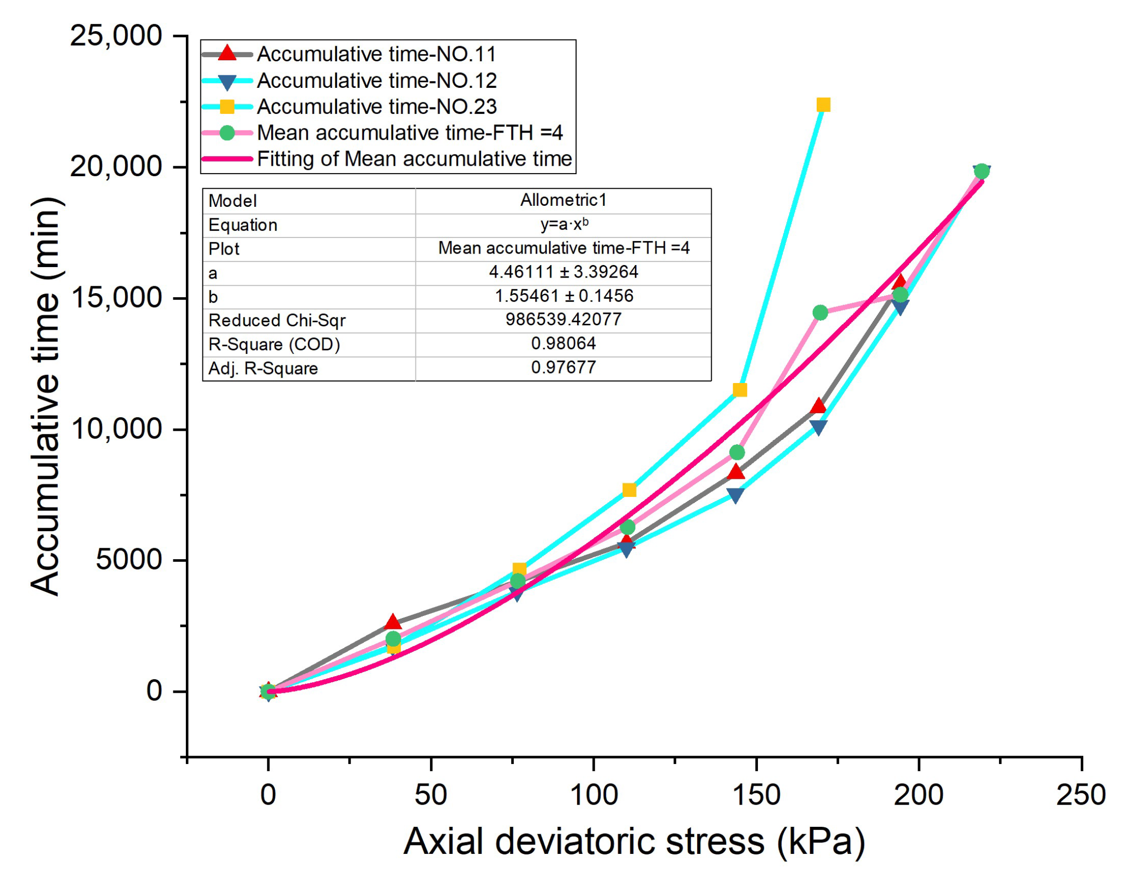
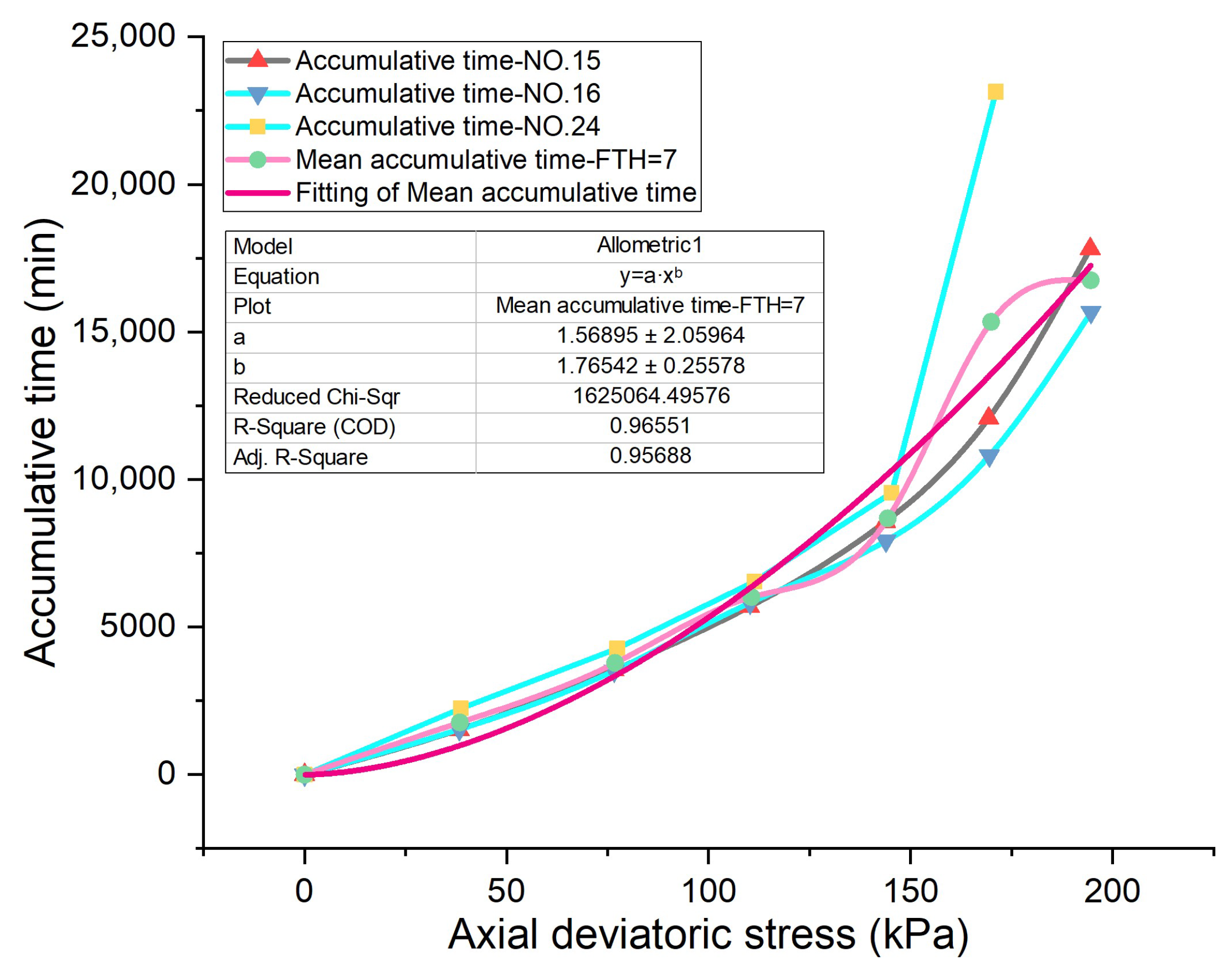
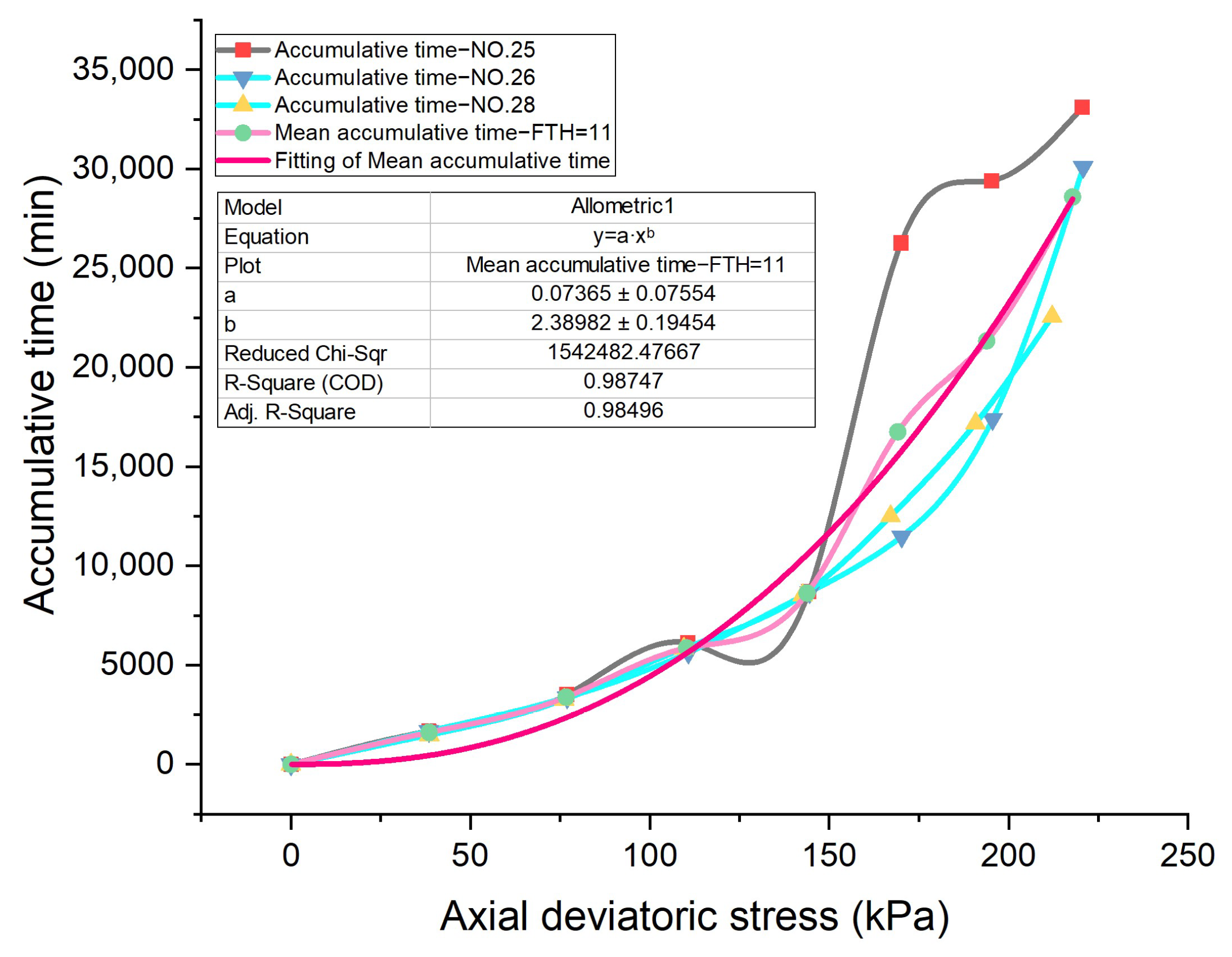
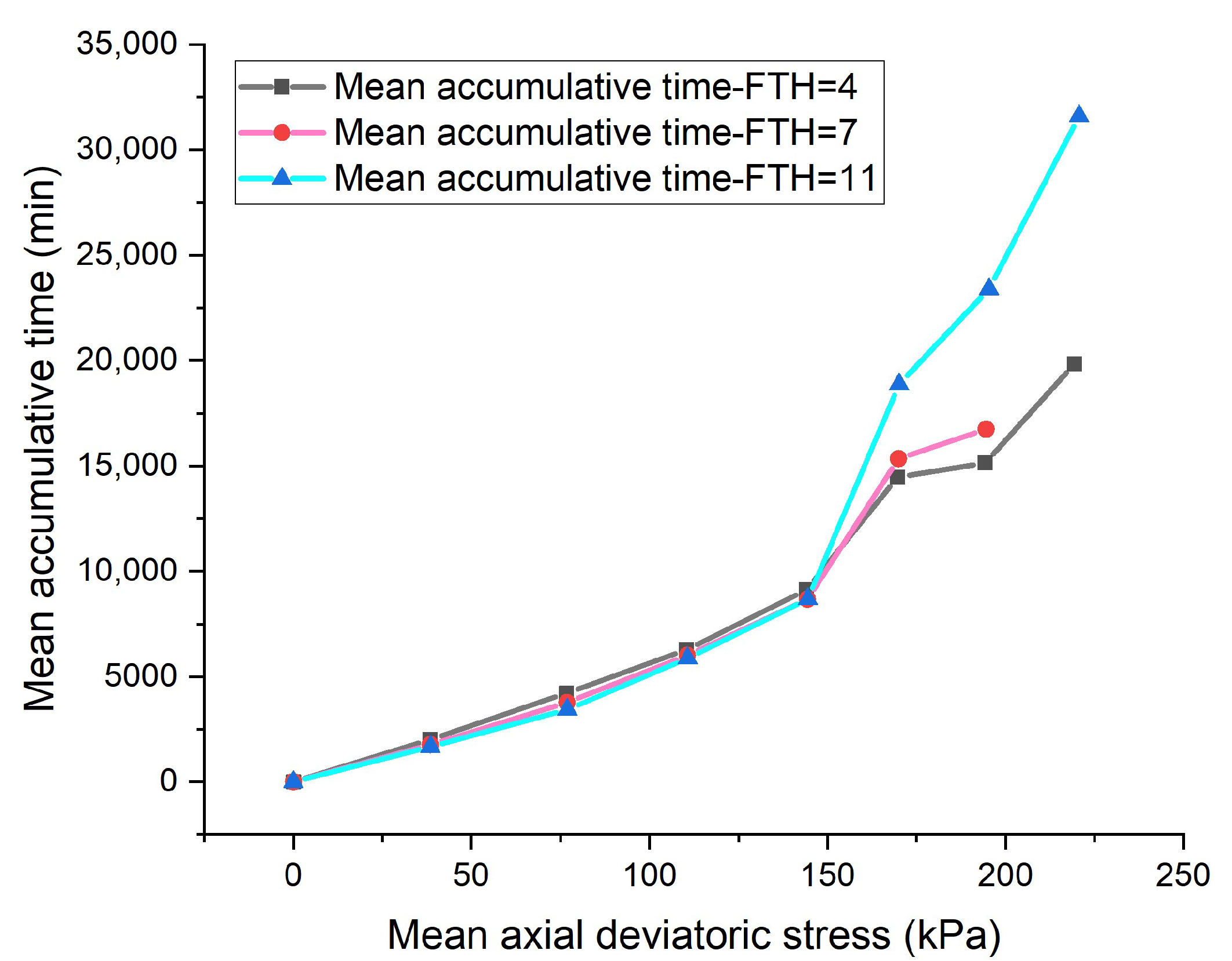
4.2. Analysis of Accumulative Time Needed for Stable Deformation When Going through Different FTHs
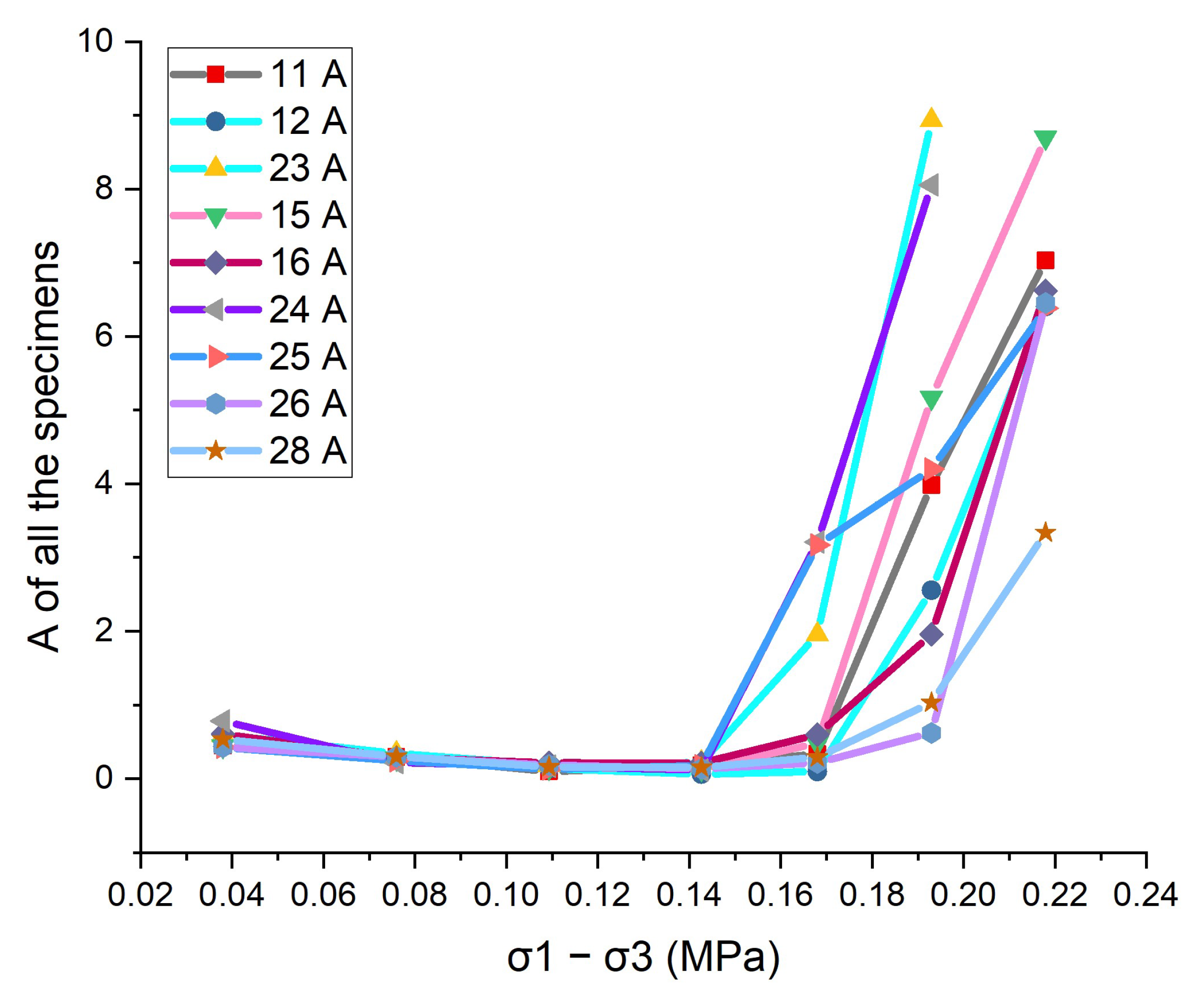
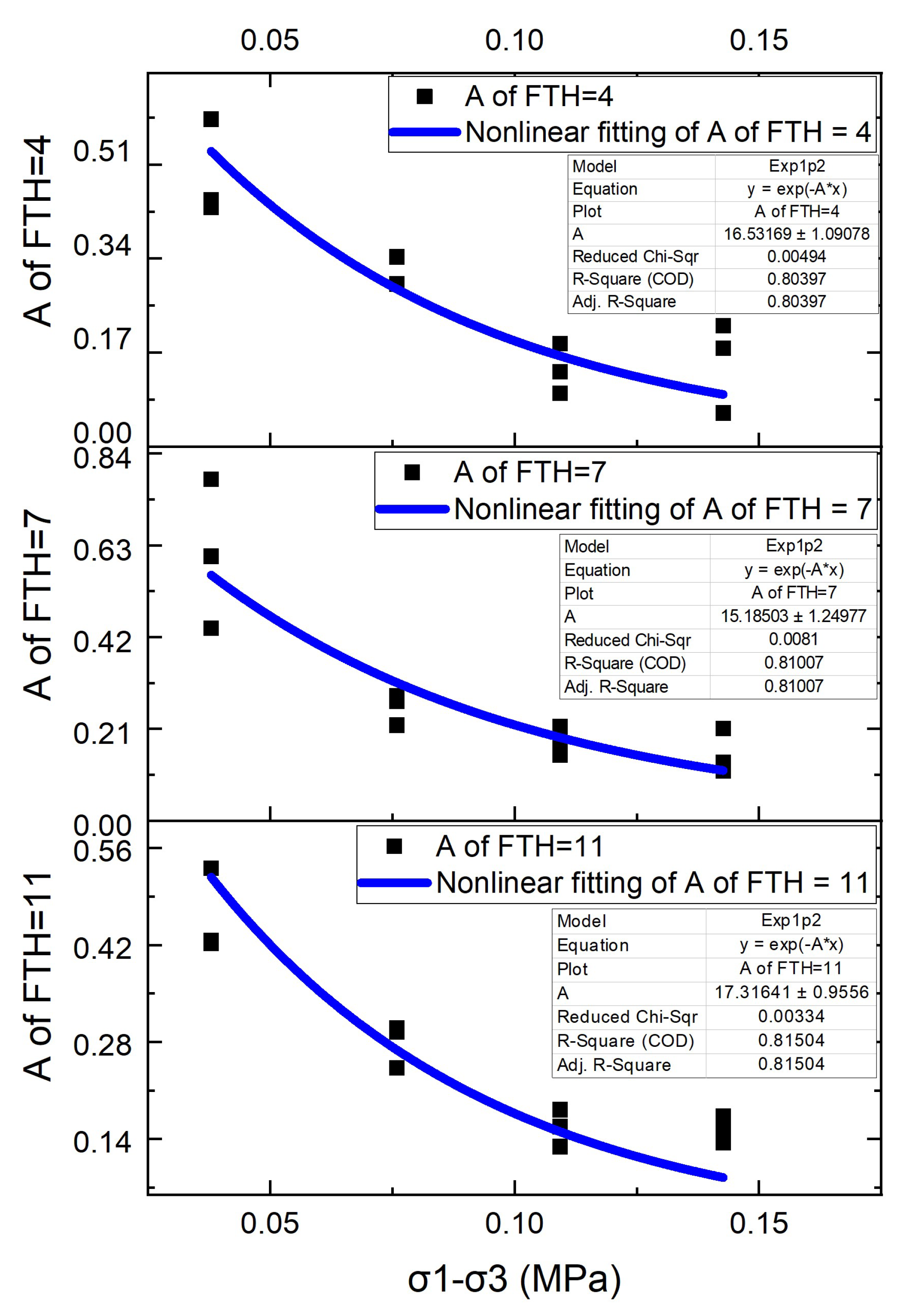
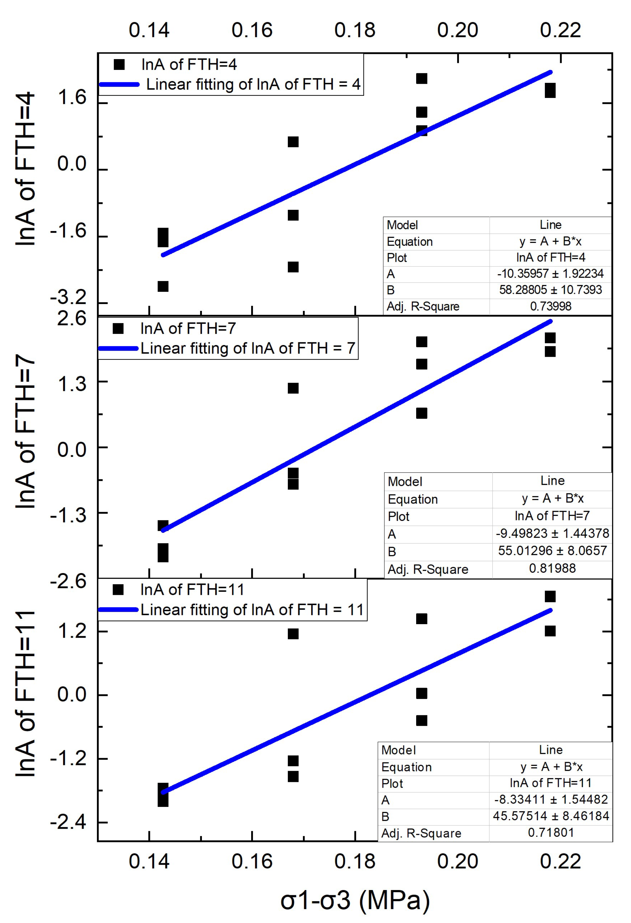
4.3. Analysis of the Effect of Axial Deviatoric Stress (ADS) on Stable Strain under 150 kPa Confining Pressure and 4, 7 and 11 FTHs
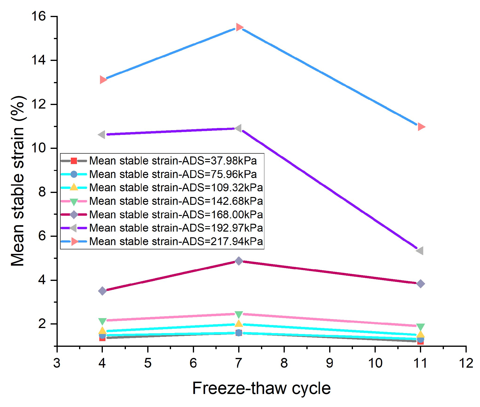
4.4. Analysis of the FTH Effect on Stable Strain under 150 kPa Confining Pressure and Preset Axial Deviatoric Stress
4.5. Analysis of Stress–Strain–Time Relationship under Varied FTHs
4.5.1. The Mathematical Significance of the Empirical Stress–Strain–Time Model
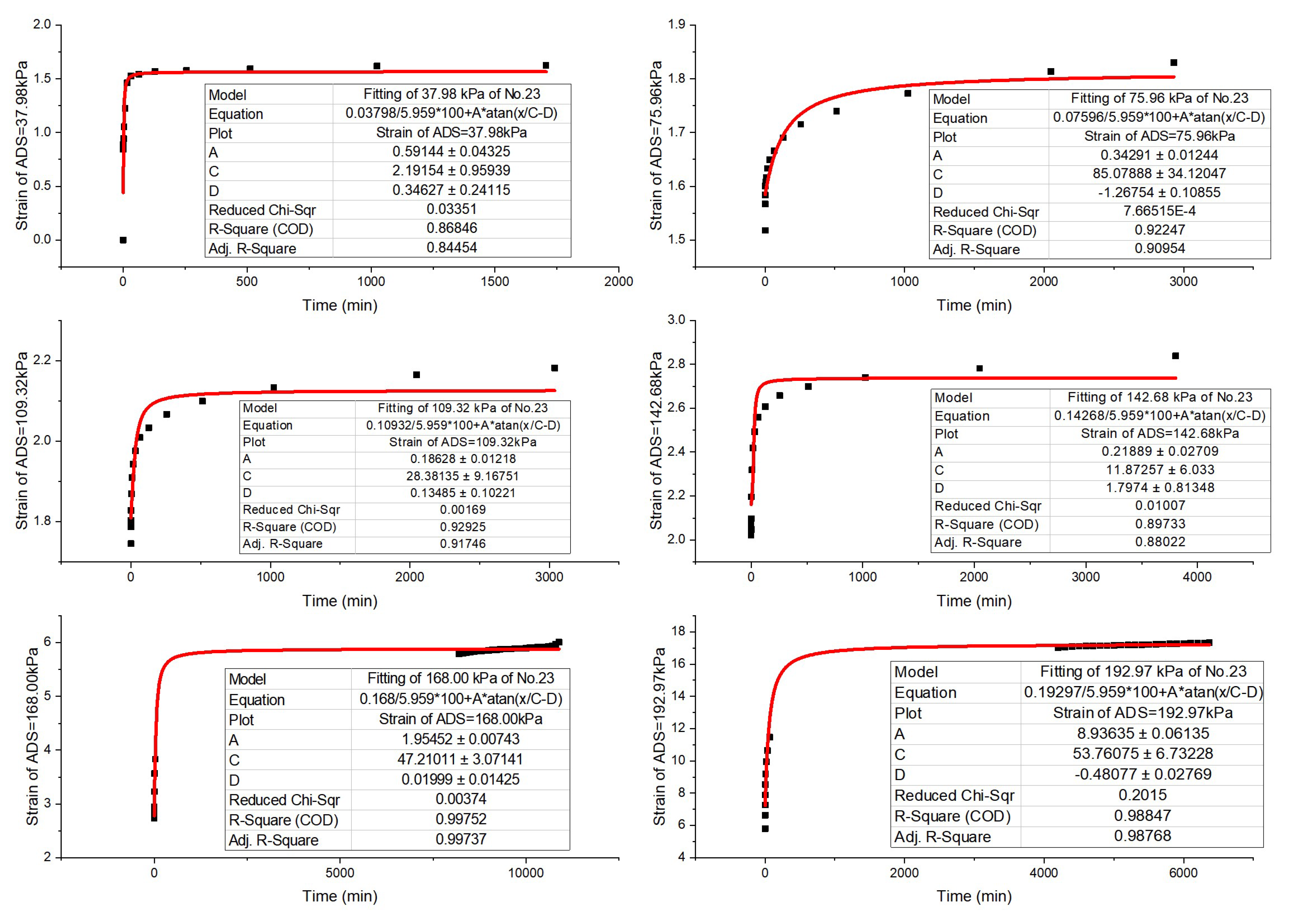
4.5.2. The Fitting Results of All the Strain–Time Curves
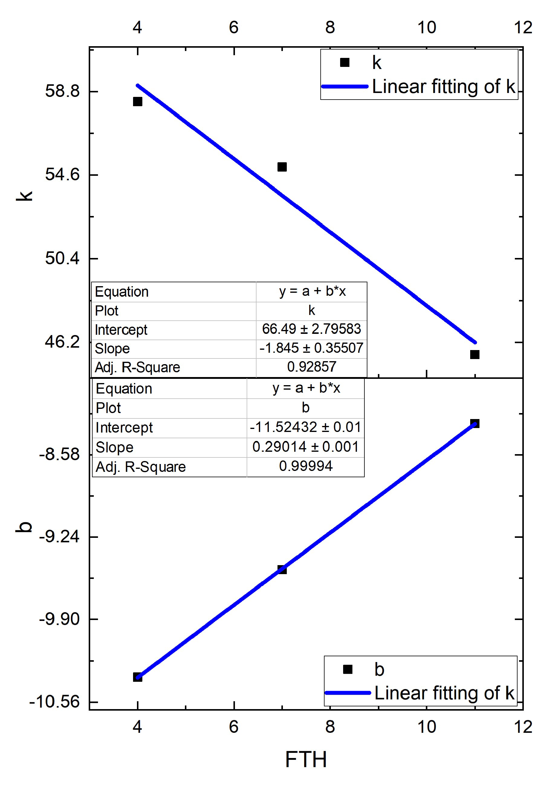
4.5.3. The Specific Expression of A
4.5.4. The Physical Significance of the Coefficients in the Stress–Strain–Time Model
5. Discussion
6. Conclusions
Author Contributions
Funding
Institutional Review Board Statement
Informed Consent Statement
Data Availability Statement
Acknowledgments
Conflicts of Interest
References
- Chamberlain, E.J.; Gow, A.J. Effect of freezing and thawing on the permeability and structure of soils. In Developments in Geotechnical Engineering; Elsevier: Amsterdam, The Netherlands, 1979; Volume 26, pp. 73–92. [Google Scholar]
- Eigenbrod, K.D. Effects of cyclic freezing and thawing on volume changes and permeabilities of soft fine-gained soils. Can. Geotech. J. 1996, 33, 529–537. [Google Scholar] [CrossRef]
- Viklander, P.; Eigenbrod, D. Stone movements and permeability changes in till caused by freezing and thawing. Cold Reg. Sci. Technol. 2000, 31, 151–162. [Google Scholar] [CrossRef]
- Yang, C.S.; He, P.; Cheng, G.D.; Zhu, Y.L.; Zhao, S.P. Testing study on influence of freezing and thawing on dry density and water content of soil. Chin. J. Rock Mech. Eng. 2003, 22, 2695–2699. [Google Scholar]
- Shi, Y.H. Study on Stability of the Subgrade under Train Loading and Freeze-Thaw. Ph.D. Thesis, Beijing Jiaotong University, Beijing, China, 2011. Available online: https://kns.cnki.net/KCMS/detail/detail.aspx?dbname=CDFD0911&filename=1011102657.nh (accessed on 28 June 2011).
- Wang, D.Y.; Ma, W.; Chang, X.X.; Sun, Z.Z.; Feng, W.J.; Zhang, J.W. Physico-mechanical properties changes of Qinghai-Tibet clay due to cyclic freezing and thawing. Chin. J. Rock Mech. Eng. 2005, 24, 4313–4319. [Google Scholar]
- Dai, W.T.; Wei, H.B.; Liu, H.B.; Gao, Y.P. Dynamic damage model of silty clay after freeze–thaw cycles. Jilin Daxue Xuebao (Gongxueban)/J. Jilin Univ. (Eng. Technol. Ed.) 2007, 37, 790–793. [Google Scholar]
- Li, X.J. Study on Creep Mechanical Characteristics of Artificially Frozen Soft Sandstone in Cretaceous Stratum. Master’s Thesis, Xi’an University of Science and Technology, Xi’an, China, 2019. Available online: https://kns.cnki.net/KCMS/detail/detail.aspx?dbname=CMFD202001&filename=1019618571.nh (accessed on 18 June 2019).
- Yang, X.R.; Jiang, A.N. Experimental study on creep properties of freeze-thawed gneiss based on nuclear magnetic resonance. J. Exp. Mech. 2020, 35, 463–471. [Google Scholar]
- Zhang, F.R.; Jiang, A.N.; Yang, X.R.; Shen, F.Y. Experimental and model research on shear creep of granite under freeze-thaw cycles. Rock Soil Mech. 2020, 41, 509. [Google Scholar]
- Wu, Y. Study on Strength, Damage and Creep Characteristics of Rock-Like Materials under Freeze-Thaw Cycle. Ph.D. Thesis, Qingdao University of Science & Technology, Qingdao, China, 2018. Available online: https://kns.cnki.net/KCMS/detail/detail.aspx?dbname=CDFDLAST2018&filename=1018831444.nh (accessed on 20 March 2018).
- Zhu, J. Study of the Damage and Creep Properties of Frozen Soft Rock of Cretaceous Formation. Ph.D. Thesis, Anhui University of Science and Technology, Huainan, China, 2014. Available online: https://kns.cnki.net/KCMS/detail/detail.aspx?dbname=CDFD1214&filename=1014382902.nh (accessed on 1 June 2014).
- Chen, G.Q.; Jian, D.H.; Chen, Y.H. Shear creep characteristics of red sandstone after freeze-thaw with different water contents. Chin. J. Geotech. Eng. 2021, 43, 661–669. [Google Scholar] [CrossRef]
- Feng, X.Z.; Qin, N.; Cui, L.Z.; Ge, Q.; Wang, Y.Y. Experimental study on triaxial creep behavior of yellow sandstone under the coupling of chemical solution and freeze-thaw cycle. Chin. J. Appl. Mech. 2021, 38, 1383–1391. [Google Scholar]
- Li, J.L.; Zhu, L.Y.; Zhou, K.P.; Chen, H.; Gao, L.; Lin, Y.; Shen, Y.J. Non-linear creep damage model of sandstone under freeze-thaw cycle. J. Cent. South Univ. 2021, 28, 954–967. [Google Scholar] [CrossRef]
- Zhang, H.; Yuan, C.; Yang, G.; Wu, L.; Peng, C.; Ye, W.; Shen, Y.; Moayedi, H. A novel constitutive modelling approach measured under simulated freeze–thaw cycles for the rock failure. Eng. Comput. 2021, 37, 779–792. [Google Scholar] [CrossRef]
- Song, Y.; Che, Y.; Zhang, L.; Ren, J.; Chen, S.; Hu, M. Triaxial creep behavior of red sandstone in freeze-thaw environments. Geofluids 2020, 2020, 6641377. [Google Scholar] [CrossRef]
- Wang, J.W. Study on the Structure Evolution of Deep Soil under Freeze-Thaw Effect and Its Influence on Creep Deformation. Master’s Thesis, China University of Mining and Technology, Xuzhou, China, 2018. Available online: https://kns.cnki.net/KCMS/detail/detail.aspx?dbname=CMFD201901&filename=1018826990.nh (accessed on 25 May 2018).
- Guan, S. The Experiment of Direct Shear Creep of Clay under Freeze-Thaw Cycle. Master’s Thesis, Liaoning Technical University, Fuxin, China, 2015. Available online: https://kns.cnki.net/KCMS/detail/detail.aspx?dbname=CMFD201901&filename=1018267707.nh (accessed on 29 December 2015).
- Cao, H.L. Study of Deformation and Wave Velocity Characteristics of Deep Clay with Different Stress Paths under Freeze-Thaw Conditions. Master’s Thesis, China University of Mining and Technology, Xuzhou, China, 2020. [Google Scholar] [CrossRef]
- Ming, F.; Ren, X.L.; Wang, J.G.; Zhou, Z.W.; Liu, E.L.; Yu, Q.H. Effect of freeze–thaw cycles on the deformation behavior of gravelly soil in the 300 m-high earth core rockfill dam. Environ. Earth Sci. 2021, 80, 297. [Google Scholar] [CrossRef]
- Xia, M.L. Deformation Characteristics and Numerical Analysis of Subgrade Soil under Freezing and Thawing Cycle. Master’s Thesis, Jilin University, Jilin, China, 2020. [Google Scholar] [CrossRef]
- Gao, Z. Research on the creep of subgrade soil after freeze-thaw cycle. Resour. Environ. Inf. Eng. 2021, 36, 64–67. [Google Scholar] [CrossRef]
- Wang, L.N. Train-Induced Dynamic Response and Permanent Deformation of Embankment in Permafrost Region along Qinghai-Tibet Railway. Ph.D. Thesis, Harbin Institute of Technology, Harbin, China, 2013. [Google Scholar]
- Zhou, Z.; Ma, W.; Zhang, S.; Mu, Y.; Li, G. Effect of freeze-thaw cycles in mechanical behaviors of frozen loess. Cold Reg. Sci. Technol. 2018, 146, 9–18. [Google Scholar] [CrossRef]
- Ma, W.; Wu, Z.W.; Zhang, C.Q. Strength and yield criteria of frozen soil. J. Glaciol. Geocryol. 1993, 15, 129–133. [Google Scholar]
- Lei, H.; Song, Y.; Qi, Z.; Liu, J.; Liu, X. Accumulative plastic strain behaviors and microscopic structural characters of artificially freeze-thaw soft clay under dynamic cyclic loading. Cold Reg. Sci. Technol. 2019, 168, 102895. [Google Scholar] [CrossRef]
- Xu, X.; Zhang, W.; Fan, C.; Lai, Y.; Wu, J. Effect of freeze–thaw cycles on the accumulative deformation of frozen clay under cyclic loading conditions: Experimental evidence and theoretical model. Road Mater. Pavement Des. 2021, 22, 925–941. [Google Scholar] [CrossRef]
- Wang, M.; Meng, S.; Yuan, X.; Sun, Y.; Zhou, J. Experimental validation of vibration-excited subsidence model of seasonally frozen soil under cyclic loads. Cold Reg. Sci. Technol. 2018, 146, 175–181. [Google Scholar] [CrossRef]
- Ma, W.; Wang, D.Y. Frozen Soil Mechanics; Science Press: Beijing, China, 2014; pp. 345–348. [Google Scholar]
- Sun, J. Rheology of Geotechnical Materials and Its Engineering Application; China Construction Industry Press: Beijing, China, 1999; pp. 26–27. [Google Scholar]
- Wong, S.T.; Ong, D.E.; Robinson, R.G. Behaviour of MH silts with varying plasticity indices. Geotech. Res. 2017, 4, 118–135. [Google Scholar] [CrossRef] [Green Version]
- Sun, G.S.; Zheng, D.T. Soft Soil Foundation and Underground Engineering; China Construction Industry Press: Beijing, China, 1984; pp. 38–49. [Google Scholar]
- Tan, T.K.; Kang, W.F. Locked in stresses, creep and dilatancy of rocks, and constitutive equations. Rock Mech. 1980, 13, 5–22. [Google Scholar] [CrossRef]
- Zhai, Y.; Wang, Y.; Dong, Y. Modified Mesri Creep Modelling of Soft Clays in the Coastal Area of Tianjin (China). Teh. Vjesn. Tech. Gaz. 2017, 24, 1113–1121. [Google Scholar] [CrossRef] [Green Version]
- Zhou, H.W.; Xie, H.P.; Zuo, J.P. Developments in researches on mechanical behaviors of rocks under the condition of high ground pressure in the depths. Adv. Mech. 2005, 35, 91–99. [Google Scholar]
- Zhao, Y.; Zhang, L.; Wang, W.; Liu, Q.; Tang, L.; Cheng, G. Experimental study on shear behavior and a revised shear strength model for infilled rock joints. Int. J. Geomech. 2020, 20, 04020141. [Google Scholar] [CrossRef]
- Peng, K.; Liu, Z.; Zou, Q.; Wu, Q.; Zhou, J. Mechanical property of granite from different buried depths under uniaxial compression and dynamic impact: An energy-based investigation. Powder Technol. 2020, 362, 729–744. [Google Scholar] [CrossRef]
- Wu, D.S.; Meng, L.B.; Li, T.B.; Lin, L. Study of triaxial rheological property and long-term strength of limestone after high temperature. Rock Soil Mech. 2016, 37, 183–191. [Google Scholar]
- Sun, F.W. Soil creep and earth dam stability. Northwest. Geol. 1999, 32, 55–57. (In Chinese) [Google Scholar]
- Yang, R.H. Study on Analysis and Evaluation to the Stability of Slope Embankment in Permafrost Regions of Qinghai-Tibet Railway in Operating Period. Ph.D. Thesis, China Academy of Railway Sciences, Beijing, China, 2010. Available online: https://kns.cnki.net/KCMS/detail/detail.aspx?dbname=CDFD1214&filename=1012566691.nh (accessed on 28 June 2010).


| Source of Rock and Soil | Description of Rock and Soil | Remolded (Re) or Undisturbed (Un) | Water Content (%) | and e Information | Temperature (°C) and Time (h) of F (Freeze)/TH (Thaw) | FTHs | Creep Test Type Uni/Bi/Triaxial | Size of Specimen (mm) | Creep Type of Describing Model |
|---|---|---|---|---|---|---|---|---|---|
| Dayan Zani Lake Strip Mine Clay, China [19]. | Brown and sticky color, slightly powdery, basically composed of clay aggregates; fine, moist, soft plastic, with organic spots, iron streaks, and a small number of conglomerate particles in the lower part. | Re | 15, 25, 35 | ρ = 2.083 g/cm3 = 2.674 e = 0.577 | −47~+20 | 0, 1, 3, 6, 10, 15 | Direct shearing creep test | H20/D61.8 | Attenuation creep |
| Rock-like materials made of shale as raw rock, and made of cement, river sand and fly ash [11]. | The fly ash content is m = 0%, 10%, 20%, 30% | Re | Saturated | −20~+20 6 h F/6 h TH | 0, 5, 10, 20, 40, 60 | Uniaxial creep test | H100/D50 | Non-attenuation creep | |
| Silty clay and clay from G25 highway subgrade in Jilin, Northeast China [22]. | According to the evaluation of the Cu and Cc values of the soil samples, it belongs to well-graded soil. values are 11.25, 16.88 and 23.22, respectively. | Re | 16, 17, 18, 19 | Compaction degree: 0.8, 0.85, 0.9, 0.95 and the maximum dry density: 1.985, 1.985, 1.944. Two groups of conditions make permutations and combinations | −10~room temperature 24 h F/24 h TH | 0, 3, 5, 7 | Triaxial creep test | H80/D39.1 | Non-attenuation creep |
| Red sandstone from Sichuan–Tibet railway FTH Area, China [13]. | Un | 0, 1.5, 2.4, 3.78 | −20~+40 1 h F/1 h TH | 0, 30, 60, 90, 120 | Direct shearing creep test | L50/W50 /H50 | Non-attenuation creep | ||
| Yellow sandstone mine in Zigong Area, Sichuan, China [14]. | The lithology is dense and yellow in color. The main components are anorthite (68%), quartz (18%), andesite cuttings (3%), amphibole (3%), pyroxene (2%) and cement (6%), and the cements are mainly calcite and iron oxide. | Un | Saturated | −20~+20 12 h F/12 h TH | 0, 15, 30, 45, 60 | Triaxial creep test | H100/D50 | Non-attenuation creep | |
| Gneiss in Jilin Huibai Tunnel (located in the middle section of Longgang Mountains at the western foot of Changbai Mountain), China [9]. | It is mainly composed of feldspar, quartz and various dark minerals (mica, amphibole, pyroxene, etc.), of which the content of feldspar and quartz is more than 50%. | Un | Saturated | −18~+22 6 h F/ 6 h TH | 0, 10, 20, 40, 80 | Triaxial creep test | H100/D50 | Non-attenuation creep | |
| Granite in the tunnel of Jilin Huibai (Huinan-Baishan Expressway Tunnel), China [10]. | Gray-white granite; the main components are quartz, potassium feldspar and acid plagioclase, and the secondary minerals are biotite and amphibole. | Un | Saturated | −20~+20 12 h F/12 h TH | 0, 10, 30, 50, 70 | Shearing creep test | L200/W100 /H200 | Non-attenuation creep | |
| Road subgrade soil under construction in a seasonally frozen area in Liaoning, China [23]. | Re | −20~room temperature 48 h F/48 h TH | 0, 4, 8, 12 | Triaxial creep test | Standard size | Non-attenuation creep | |||
| Quartz sandstone from Gansu province, China [15]. | Un | Saturated | ρ = 2.14 g/cm3 | −10~+204 h F/4 h TH | 0, 5, 10 | Uniaxial compression creep test | H100/D50 | Non-attenuation creep | |
| Gravel and soil collected from the Lianghekou Hydropower Station, China [21]. | Re | 8 | Dry density = 2200 kg/m3 | −10~+20 24 h F/12 h TH | 0, 1, 2, 5, 10 | Confined compression creep test | H200/D300 | Non-attenuation creep | |
| Fresh and unbroken red sandstone [16]. | Un | Saturated | −20~+20 3 h F/3 h TH | 5, 10, 20, 40 | Triaxial compression creep test | H100/D50 | |||
| Red sandstone from the Dafosi Coal Mine, the Binchang Mining Area, Jurassic Coalfield, Huanglong, Shaanxi Province, China [17]. | The rock formations consist of mostly thick, weak, medium- to fine-grained sandstones. The sampled rock layer is light brownish-red fine- to medium-grained feldspar quartz sandstone, mainly composed of quartz, plagioclase, potash feldspar and calcite. | Un | Saturated, 5.31% | Dry density = 2.24 g/cm3 Saturated density = 2.35 g/cm3 Porosity = 9.6% | −20~+20 12 h F/12 h TH | 0, 1, 5, 9, 13 | Triaxial compression tests and multilevel loading and unloading triaxial creep tests | H100/D50 | |
| Qinghai–Tibetan clay, from the Beiluhe test site along the Qinghai–Tibetan highway [28]. | Plastic limit = 16.5%, Liquid limit = 28.2%, Plastic index = 11.7. | Un | 21.4 | Maximum dry density = 1.82 g/cm3 | −20~+20 | 0, 1, 2, 4, 6, 8, 10 | Dynamic triaxial compression test | H100/D50 | |
| Soft clay collected from the construction site of the railway station of metro line 1 in Tianjin at a depth of 10–15 m [27]. | Cohesive force c = 1.64 kPa, Plastic limit wp = 20.7%, Liquid limit wL = 34.2%. | Re | 28.2 (saturated) | ρ = 1.82 g/cm3 Void ratio e = 1.17 | Respectively, −3, −7, −10, −15, −20, −25, −30~+20 10 h F/24 h TH | 0, 1 | Dynamic triaxial compression test | H80/D39.1 | |
| Loess from Jiuzhoutai town of Lanzhou, China [25]. | Liquid limit = 17.4%, Plastic limit = 25.7%. | Re | 16.5 (initial) | Dry unit weight = 17.8 kg/m3 | −6~+15 −12~+15 12 h F/12 h TH | 0, 3, 6, 9, 12 | Triaxial compression creep test | H125/D62 |
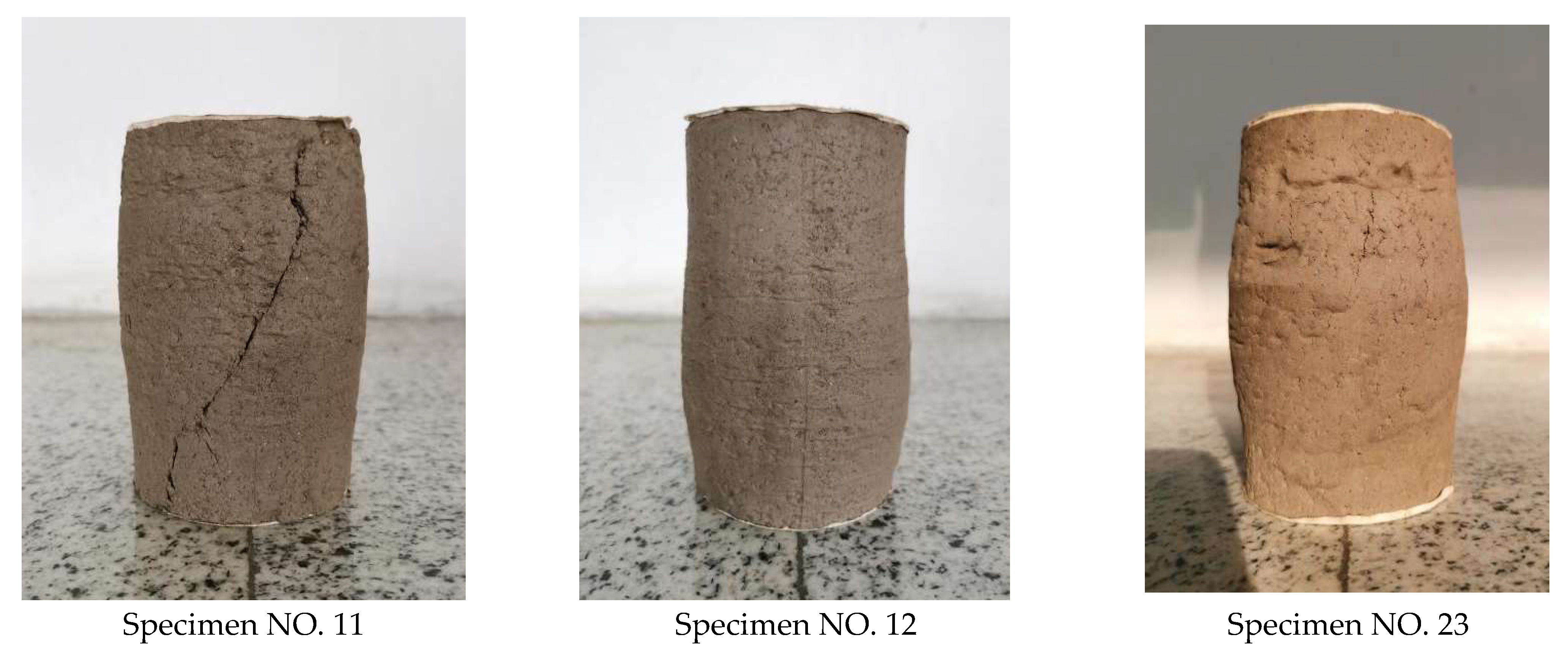
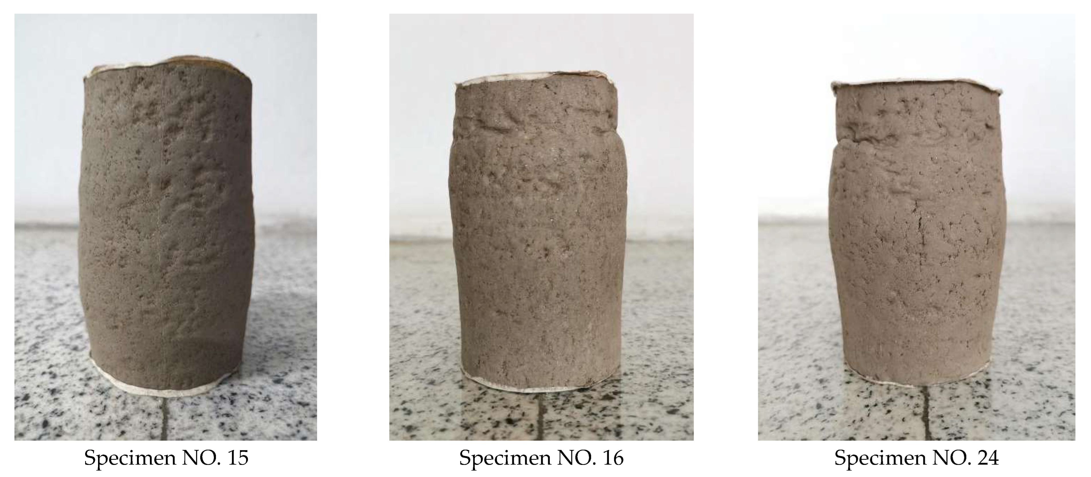
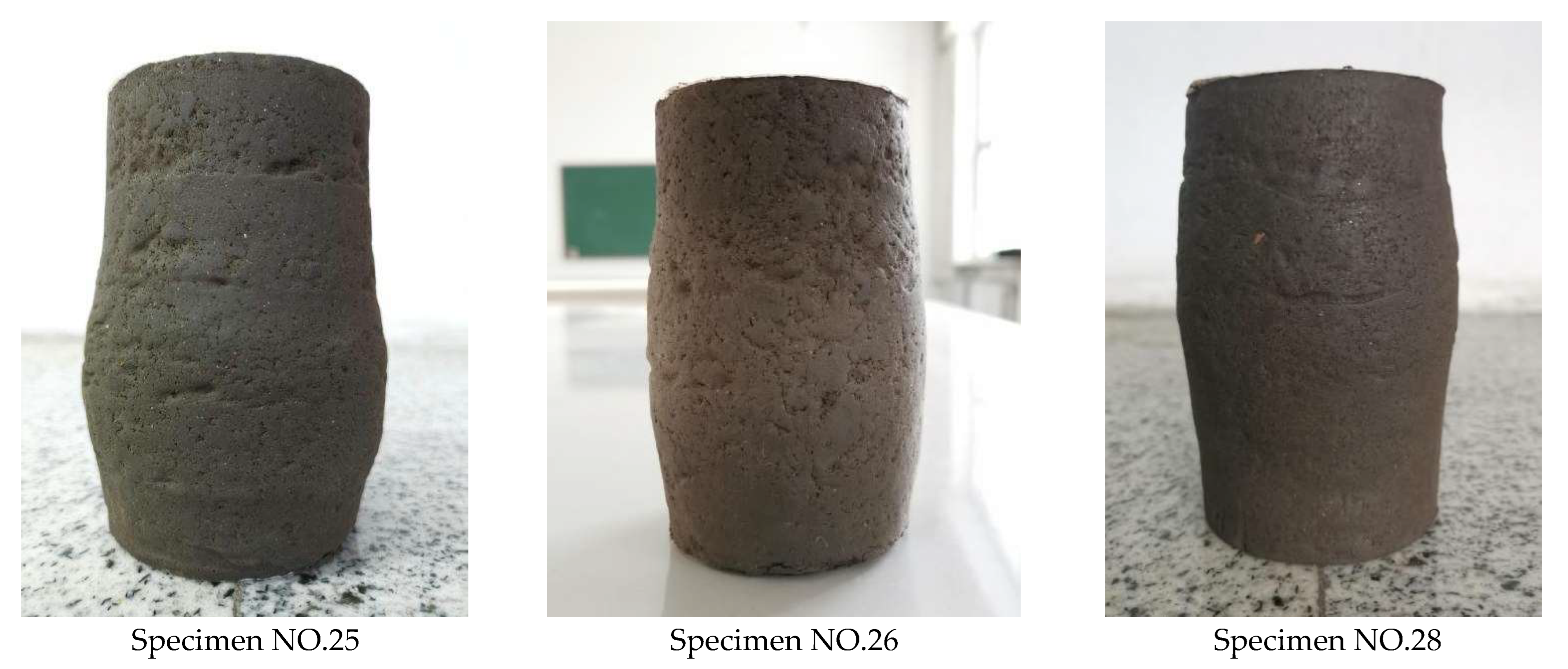
| No. | Freeze–Thaw Cycles (FTHs) | /kPa | Initial Average Diameter (D)/mm | Initial Height (H)/mm | Mass (M)/g | Moisture Content ()/% |
|---|---|---|---|---|---|---|
| 11 | 4 | 150 | 61.585 | 122.50 | 651.5 | 23.45 |
| 12 | 4 | 150 | 61.605 | 122.06 | 652.9 | 22.23 |
| 23 | 4 | 150 | 61.320 | 121.76 | 653.0 | 23.79 |
| 15 | 7 | 150 | 61.570 | 122.66 | 652.9 | 22.13 |
| 16 | 7 | 150 | 61.540 | 120.40 | 654.2 | 22.57 |
| 24 | 7 | 150 | 61.245 | 120.60 | 653.6 | 22.97 |
| 25 | 11 | 150 | 61.440 | 121.68 | 652.3 | 23.55 |
| 26 | 11 | 150 | 61.405 | 122.86 | 653.3 | 23.25 |
| 28 | 11 | 150 | 61.310 | 122.34 | 652.9 | 23.40 |
| No. | /kPa | /kPa |
|---|---|---|
| 1 | 100 | 227.63 |
| 2 | 150 | 250.40 |
| 3 | 200 | 264.15 |
| No. | /kPa | Dramatically Increasing Deformation Stress Level/kPa |
|---|---|---|
| 11 | 109.32~168.00 | - |
| 12 | 109.32~192.97 | 192.97, 217.94 |
| 23 | 75.96~168.00 | 168.00, 192.97 |
| 15 | 109.32~168.00 | - |
| 16 | 75.96~168.00 | 217.94 |
| 24 | 75.96~168.00 | 168.00 |
| 25 | 109.32~168.00 | 168.00 |
| 26 | 109.32~192.97 | 217.94 |
| 28 | 109.32~192.97 | - |
| No. | FTH | E/MPa | /MPa |
|---|---|---|---|
| 11 | 4 | 7.452 | 8.140 |
| 12 | 4 | 11.008 | |
| 23 | 4 | 5.959 | |
| 15 | 7 | 9.518 | 7.038 |
| 16 | 7 | 4.613 | |
| 24 | 7 | 6.983 | |
| 25 | 11 | 8.174 | 8.791 |
| 26 | 11 | 9.369 | |
| 28 | 11 | 8.831 |
| /kPa | 11 A | 12 A | 23 A | 15 A | 16 A | 24 A | 25 A | 26 A | 28 A |
|---|---|---|---|---|---|---|---|---|---|
| 37.98 | 0.4454 | 0.4325 | 0.5914 | 0.4404 | 0.6048 | 0.7808 | 0.4221 | 0.4264 | 0.5309 |
| 75.96 | 0.2941 | 0.2945 | 0.3429 | 0.2734 | 0.2851 | 0.2180 | 0.2425 | 0.2943 | 0.3003 |
| 109.32 | 0.0966 | 0.1351 | 0.1863 | 0.1502 | 0.2147 | 0.1676 | 0.1289 | 0.1824 | 0.1580 |
| 142.68 | 0.1777 | 0.0610 | 0.2188 | 0.1333 | 0.2108 | 0.1135 | 0.1732 | 0.1347 | 0.1531 |
| 168.00 | 0.3367 | 0.0971 | 1.9545 | 0.4795 | 0.5967 | 3.2099 | 3.1692 | 0.2157 | 0.2890 |
| 192.97 | 3.9808 | 2.5552 | 8.9364 | 5.1686 | 1.9565 | 8.0530 | 4.2001 | 0.6187 | 1.0293 |
| 217.94 | 7.0337 | 6.4043 | 8.6997 | 6.6189 | 6.3806 | 6.4529 | 3.3383 |
Publisher’s Note: MDPI stays neutral with regard to jurisdictional claims in published maps and institutional affiliations. |
© 2022 by the authors. Licensee MDPI, Basel, Switzerland. This article is an open access article distributed under the terms and conditions of the Creative Commons Attribution (CC BY) license (https://creativecommons.org/licenses/by/4.0/).
Share and Cite
Qu, H.; Mu, D.; Ren, Z.; Huang, Z.; Huang, Y.; Tang, A. Stress–Strain–Time Description and Analysis of Frozen–Thawed Silty Clay under Low Stress Level. Geotechnics 2022, 2, 871-907. https://doi.org/10.3390/geotechnics2040042
Qu H, Mu D, Ren Z, Huang Z, Huang Y, Tang A. Stress–Strain–Time Description and Analysis of Frozen–Thawed Silty Clay under Low Stress Level. Geotechnics. 2022; 2(4):871-907. https://doi.org/10.3390/geotechnics2040042
Chicago/Turabian StyleQu, Haigang, Dianrui Mu, Zhenlu Ren, Ziyuan Huang, Yang Huang, and Aiping Tang. 2022. "Stress–Strain–Time Description and Analysis of Frozen–Thawed Silty Clay under Low Stress Level" Geotechnics 2, no. 4: 871-907. https://doi.org/10.3390/geotechnics2040042