
Conversion of Triaxial Compression Strain–Time Curves from Stepwise Loading to Respective Loading

Abstract
:1. Introduction
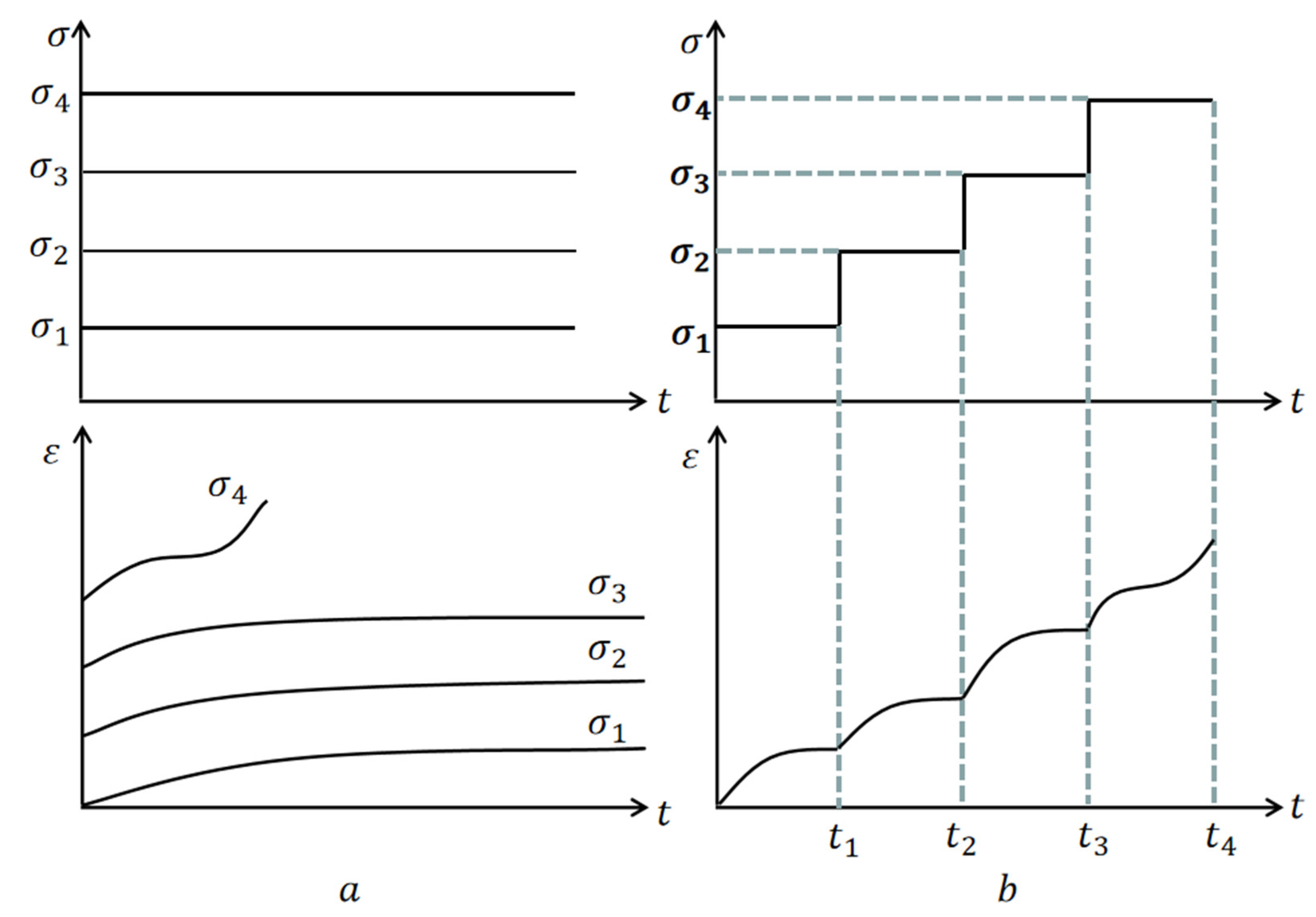
1.1. Loading Mode
1.2. Strain–Time Curves and Creep Curves
1.3. Classical Conversion Methods for Creep Curves
1.3.1. The Coordinate Translation Method (CTM)
1.3.2. Chen’s Method (Tan’s Method)
1.3.3. Sun’s Conversion Method
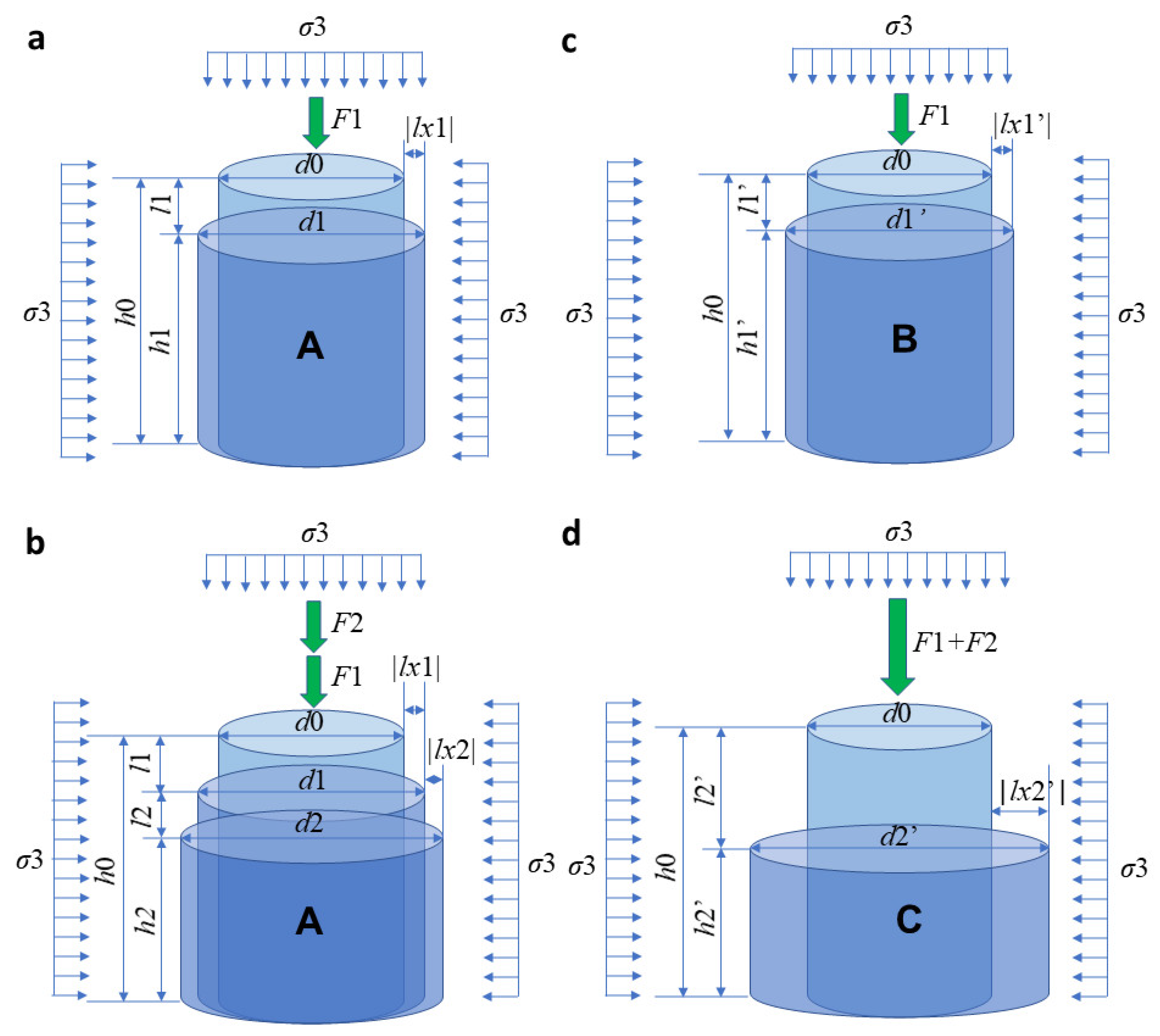
2. Method—The Revise Energy Method (REM) for the Conversion of the Strain–Time Curves
3. Experiment and Result—An Instance for the Revise Energy Method
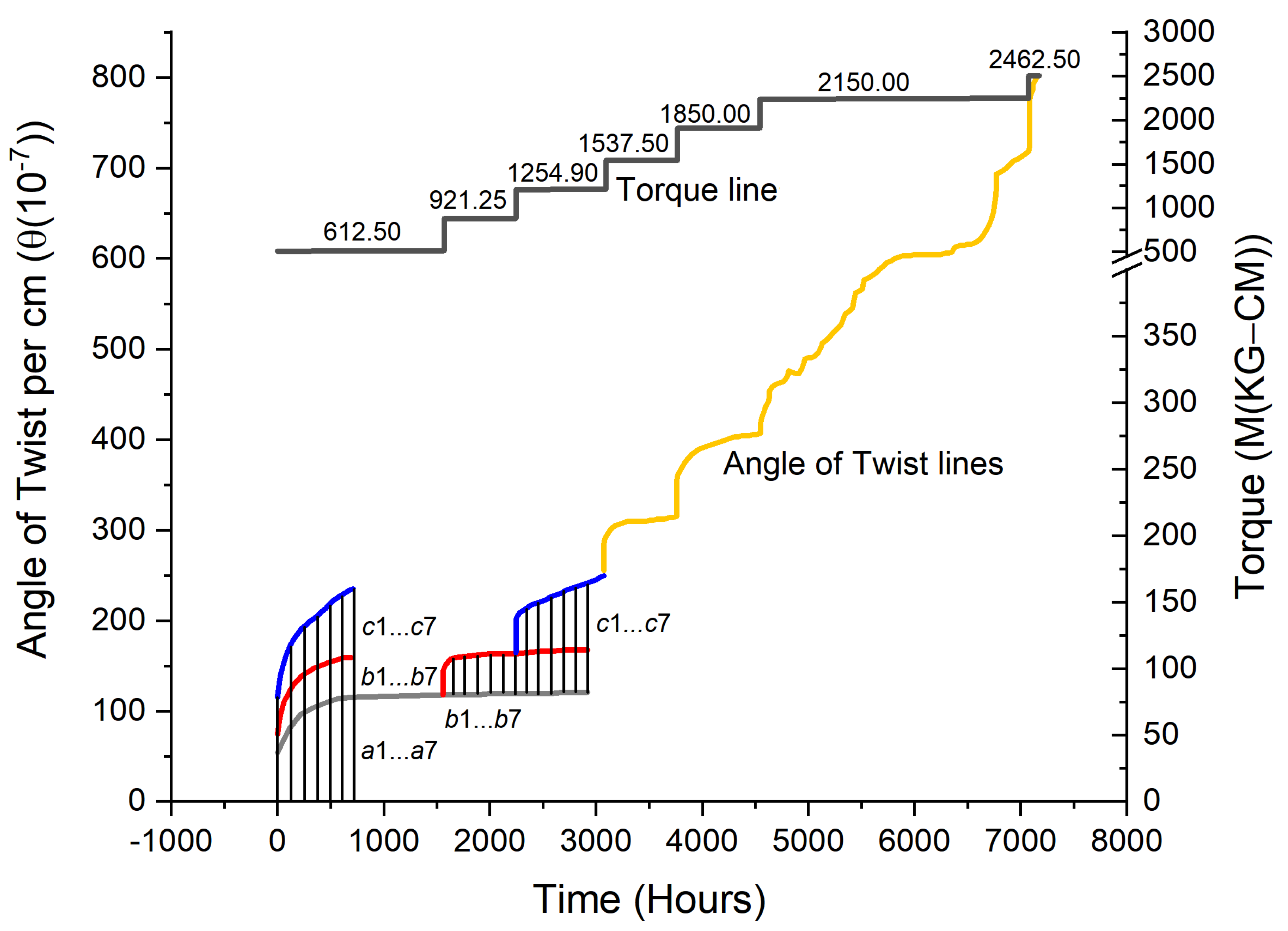
3.1. Experiment
3.2. Result
4. Discussions—Analysis of the Revise Energy Method
4.1. The Trend Analysis
4.2. The Disparity Analysis
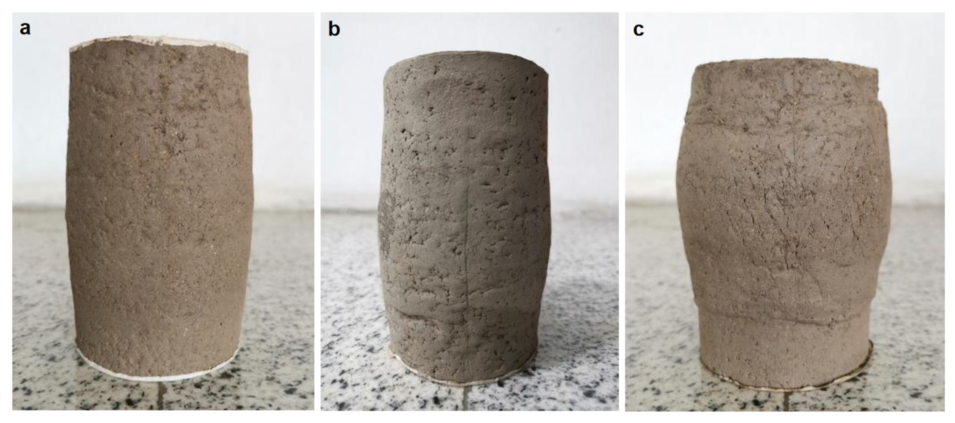
- 1
- The cylinder geometrical hypothesis is not totally applicable to the test results of specimens in shape, as in Figure 4.
- 2
- The bulk strain data used in the conversion is tested in SL, not the bulk strain tested in RL, the disparity caused by the discrepancy of bulk strain may be accumulated with the stress load increasing.
- 3
- The initial size of the specimen may not accurately be 61.8 mm × 125 mm, which will not influence the RL strain–time curve decisively but will influence the conversion of REM because d0 and h0 are vital parameters for the REM.
5. Conclusions
Author Contributions
Funding
Data Availability Statement
Conflicts of Interest
References
- Liingaard, M.; Augustesen, A.; Lade, P.V. Characterization of Models for Time-Dependent Behavior of Soils. Int. J. Géoméch. 2004, 4, 157–177. [Google Scholar] [CrossRef]
- Sun, J. Rheology of Geotechnical Materials and Its Engineering Application; China Construction Industry Press: Beijing, China, 1999. [Google Scholar]
- Zhai, Y.; Wang, Y.; Dong, Y. Modified Mesri Creep Modelling of Soft Clays in the Coastal Area of Tianjin (China). Teh. Vjesn.-Tech. Gaz. 2017, 24, 1113–1121. [Google Scholar] [CrossRef]
- Jiang, Y.Z.; Wang, R.H.; Zhu, J.B. Rheological mechanical properties of altered-rock. Mater. Res. Innov. 2015, 19, S5-349–S5-355. [Google Scholar] [CrossRef]
- Ou, Z.-F.; Fang, Y.-G. The Influence of Organic Matter Content on the Rheological Model Parameters of Soft Clay. Soil Mech. Found. Eng. 2017, 54, 283–288. [Google Scholar] [CrossRef]
- Han, B.; Fu, Q. Study on the Estimation of Rock Rheological Parameters under Multi-level Loading and Unloading Conditions. MATEC Web Conf. 2018, 213, 02003. [Google Scholar] [CrossRef]
- Li, K.-F.; Liu, R.; Qiu, C.-L.; Tan, R.-J. Consolidated Drained Creep Model of Soft Clay in Tianjin Coastal Areas; Springer: Singapore, 2018; pp. 157–165. [Google Scholar] [CrossRef]
- Wang, Z.; Wong, R.C.K. Strain-Dependent and Stress-Dependent Creep Model for a Till Subject to Triaxial Compression. Int. J. Géoméch. 2016, 16, 04015084. [Google Scholar] [CrossRef]
- Li, J.; Tang, Y.; Feng, W. Creep behavior of soft clay subjected to artificial freeze–thaw from multiple-scale perspectives. Acta Geotech. 2020, 15, 2849–2864. [Google Scholar] [CrossRef]
- Hu, K.; Shao, J.-F.; Zhu, Q.-Z.; Zhao, L.-Y.; Wang, W.; Wang, R.-B. A micro-mechanics-based elastoplastic friction-damage model for brittle rocks and its application in deformation analysis of the left bank slope of Jinping I hydropower station. Acta Geotech. 2020, 15, 3443–3460. [Google Scholar] [CrossRef]
- Zhang, G.; Chen, C.; Zornberg, J.G.; Morsy, A.M.; Mao, F. Interface creep behavior of grouted anchors in clayey soils: Effect of soil moisture condition. Acta Geotech. 2020, 15, 2159–2177. [Google Scholar] [CrossRef]
- Yao, X.; Qi, J.; Zhang, J.; Yu, F. A one-dimensional creep model for frozen soils taking temperature as an independent variable. Soils Found. 2018, 58, 627–640. [Google Scholar] [CrossRef]
- Bhat, D.; Kozubal, J.; Tankiewicz, M. Extended Residual-State Creep Test and Its Application for Landslide Stability Assessment. Materials 2021, 14, 1968. [Google Scholar] [CrossRef]
- Liu, Z.B.; Xie, S.Y.; Shao, J.F.; Conil, N. Multi-step triaxial compressive creep behaviour and induced gas permeability change of clay-rich rock. Géotechnique 2018, 68, 281–289. [Google Scholar] [CrossRef]
- Zhang, Y.Q. Research on Creep Model Test of Rockfill Material. Master’s Thesis, China Academy of Water Resources and Hydropower Sciences, Beijing, China, June 2013. [Google Scholar]
- Shen, Z.J.; Zuo, Y.M. Experimental research on rheological properties of rockfill. In Proceedings of the 6th Symposium on Soil Mechanics and Foundation Engineering of the Chinese Society of Civil Engineering, Shanghai, China, 18–22 June 1991; pp. 443–446. [Google Scholar]
- Cheng, Z.L.; Ding, H.S. Creep test for rockfill. Chin. J. Geotech. Eng. 2004, 26, 473–476. [Google Scholar]
- Zhao, L.; Gan, H.X.; Tang, W.; Tang, M.F.; Zhou, H.P. Applicability Analysis of Chen’s Method in the Research of TATB-based PBX Creep Behavior. Chin. J. Energetic Mater. 2018, 26, 608–613. [Google Scholar] [CrossRef]
- Zhao, X.; Wang, Q.; Gao, Y.; Yang, T.; He, L.; Lu, X. Indoor Rheological Test and Creep Model Analysis of Soft Soil in Qingyi River region in Wuhu Anhui. IOP Conf. Series: Earth Environ. Sci. 2019, 330, 032007. [Google Scholar] [CrossRef]
- Tan, T.K.; Kang, W.F. Locked in stresses, creep and dilatancy of rocks, and constitutive equations. Rock Mech. 1980, 13, 5–22. [Google Scholar] [CrossRef]
- Zhao, D.; Gao, Q.-F.; Hattab, M.; Hicher, P.-Y.; Yin, Z.-Y. Microstructural evolution of remolded clay related to creep. Transp. Geotech. 2020, 24, 100367. [Google Scholar] [CrossRef]
- Nie, Z. Experimental Investigation on the Long-Term Properties of Expansive Soils Subjected to Freeze-Thaw Cycling. Master’s Thesis, Harbin Institute of Technology, Harbin, China, June 2018. [Google Scholar]
- Tan, T.K. Basic Nature and Engineering Suggestions of Loess in Northwest China. Chin. J. Geotech. Eng. 1989, 4, 9–24. [Google Scholar]
- Sun, J. Rock rheological mechanics and its advance in engineering applications. Chin. J. Rock Mech. Eng. 2007, 26, 1081–1106. [Google Scholar]
- Zhang, X.W.; Wang, C.M.; Zhang, S.H. Comparative analysis of soft clay creep data processing method. J. Jilin Univ. (Earth Sci. Ed.) 2010, 40, 1401–1408. [Google Scholar] [CrossRef]
- Kishi, M.; Tani, K. Development of measuring method for axial and lateral strain distribution using CCD sensor in triaxial test. In Deformation Characteristics of Geomaterials; IS: Lyon, France, 2003; pp. 31–36. [Google Scholar] [CrossRef]
- Chu, J.; Lo, S.R.; Lee, I.K. Instability of Granular Soils under Strain Path Testing. J. Geotech. Eng. 1993, 119, 874–892. [Google Scholar] [CrossRef]
- Li, S.; Huang, X.; Wu, S.; Tian, J.; Zhang, W. Bearing capacity of stabilized soil with expansive component confined by polyvinyl chloride pipe. Constr. Build. Mater. 2018, 175, 307–320. [Google Scholar] [CrossRef]
- Zhou, P.J. Study on Shear Creep Characteristics and Model of Saturated Cohesive Soil. Master’s Thesis, Zhejiang University of Technology, Hangzhou, China, June 2018. [Google Scholar]


| Source of Soil | Sampling Depth (m) | Specific Gravity Gs | Moisture Content (%) | Void Ratio | Water Limit (%) | Plastic Limit (%) | Density (g/cm3) | Particle Gradation (mm) | ||
|---|---|---|---|---|---|---|---|---|---|---|
| >0.075 | 0.05–0.075 | <0.05 | ||||||||
| West Lake, Hangzhou, China | 15–25 | 2.74 | 28 | 0.87 | 39.2 | 22 | 1.872 | 2.69 | 3.21 | 94.1 |
| Test | Confining Pressure (kPa) | Shearing Strength (kPa) | Loading Path |
|---|---|---|---|
| 1 | 400 | 330 | 60 |
| 2 | 400 | 330 | 120 |
| 3 | 400 | 330 | 240 |
| 4 | 400 | 330 | |
| 5 | 400 | 330 |
| Figure (Loading Condition) | End Strain (%) | Disparity of Strain between RL and Converted (%) | Disparity of Strain between RL and SL (%) | ||
|---|---|---|---|---|---|
| SL Curve | RL Curve | Converted Curve | |||
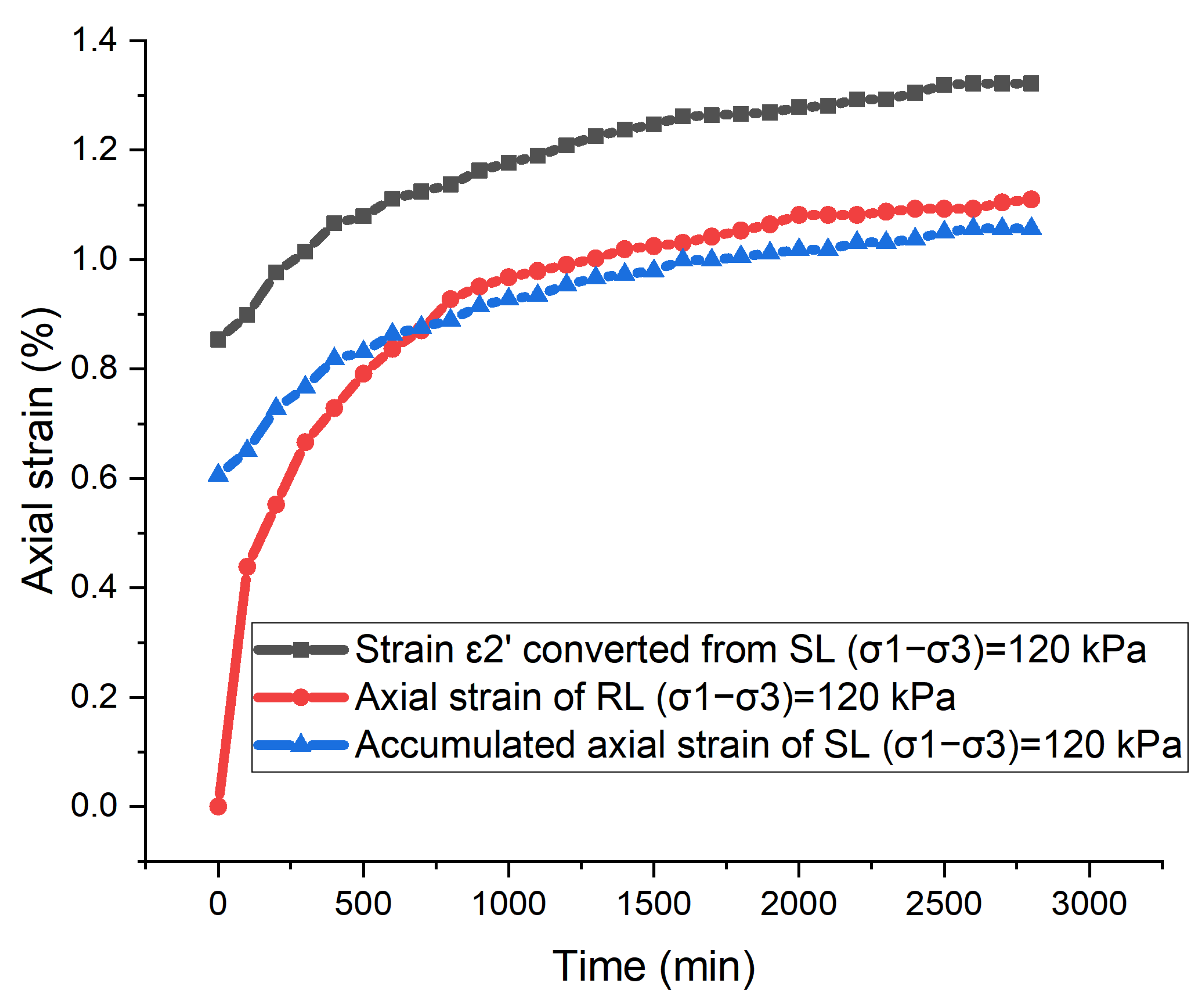
| 1 (120 kPa of Test 2 and 4) | 1.06 | 1.11 | 1.32 | 0.21 | −0.05 |
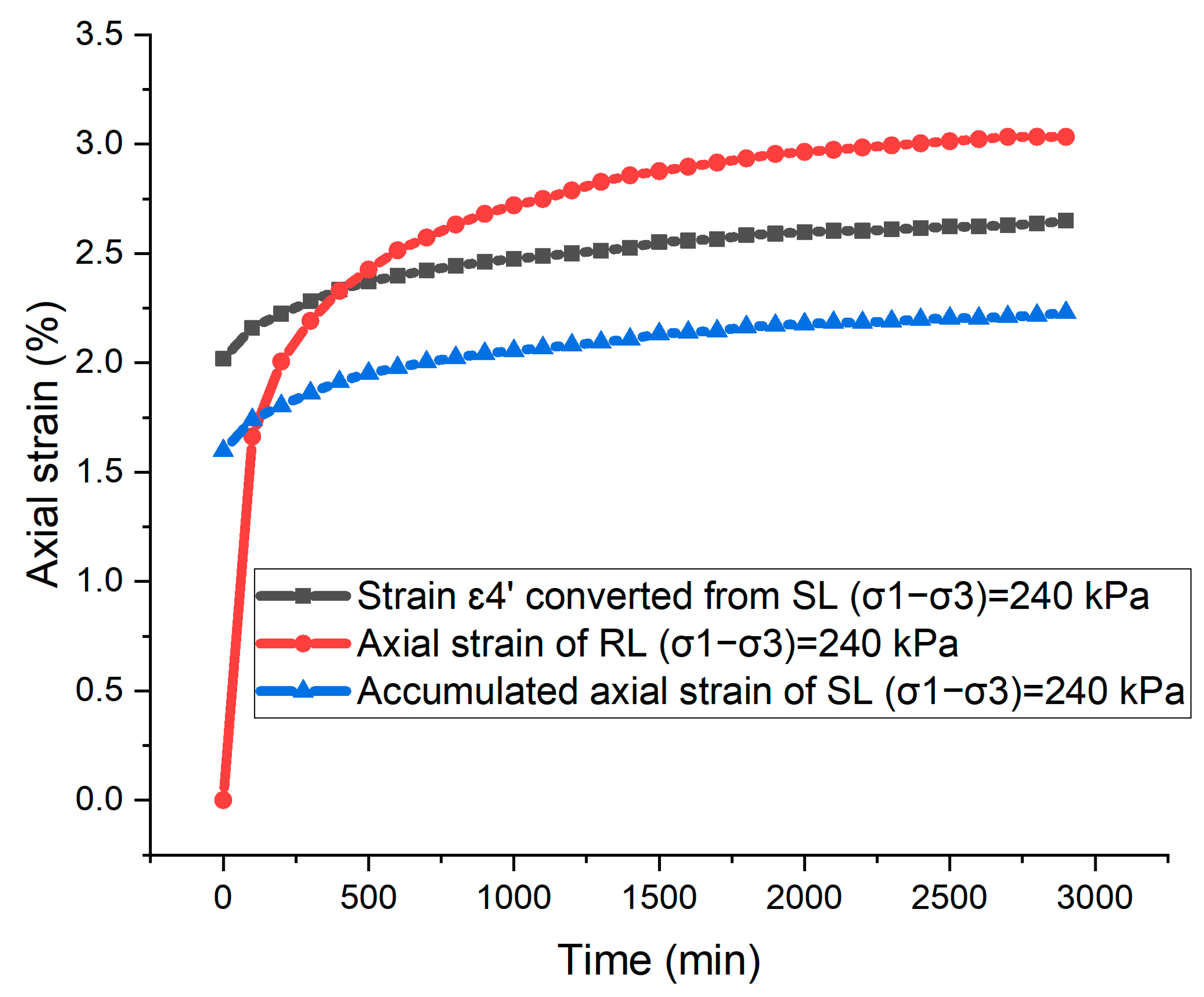
| 2 (240 kPa of Test 3 and 4) | 2.23 | 3.03 | 2.65 | −0.38 | −0.80 |
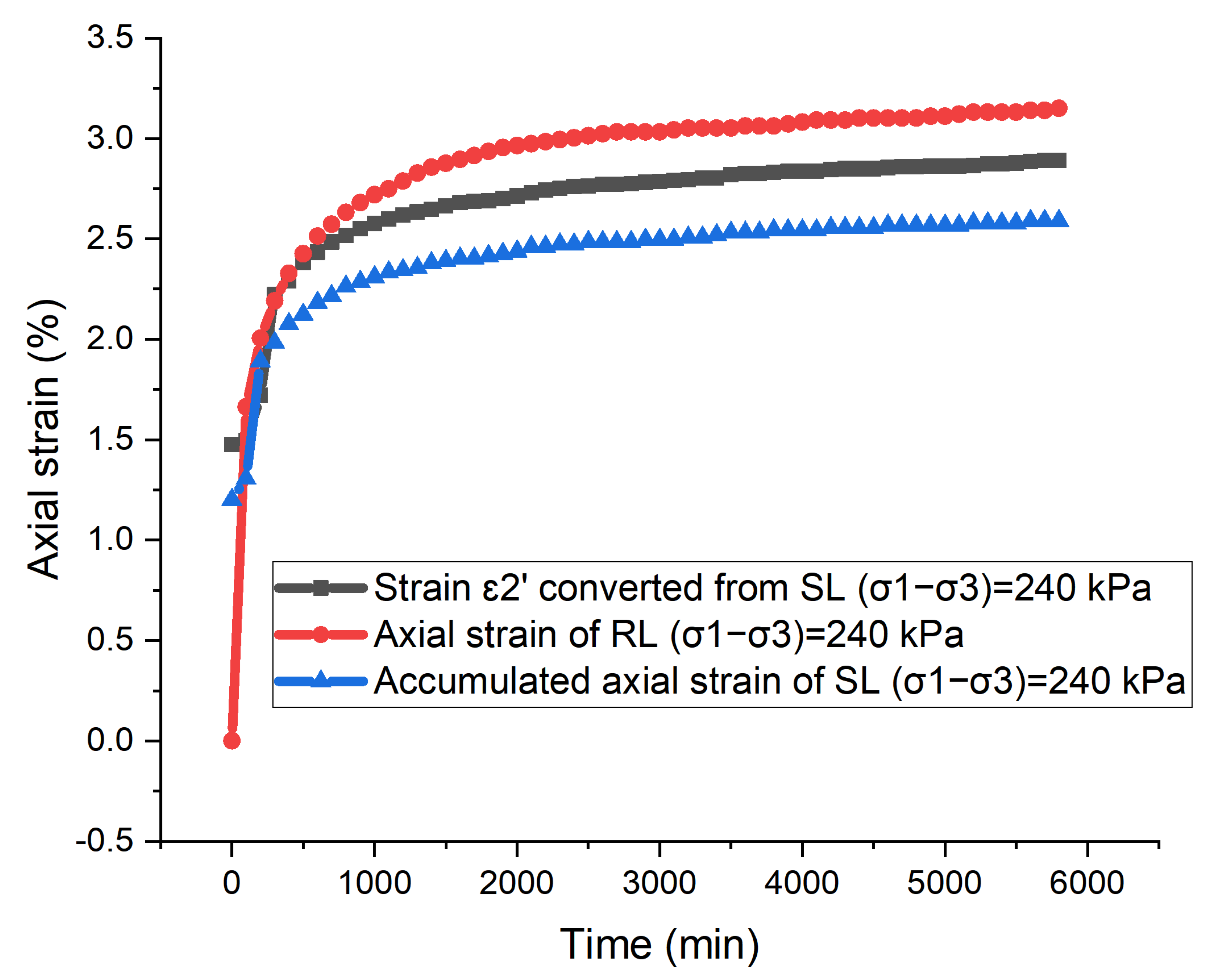
| 3 (240 kPa of Test 3 and 5) | 2.59 | 3.15 | 2.89 | −0.26 | −0.56 |
Publisher’s Note: MDPI stays neutral with regard to jurisdictional claims in published maps and institutional affiliations. |
© 2022 by the authors. Licensee MDPI, Basel, Switzerland. This article is an open access article distributed under the terms and conditions of the Creative Commons Attribution (CC BY) license (https://creativecommons.org/licenses/by/4.0/).
Share and Cite
Qu, H.; Mu, D.; Nie, Z.; Tang, A. Conversion of Triaxial Compression Strain–Time Curves from Stepwise Loading to Respective Loading. Geotechnics 2022, 2, 855-870. https://doi.org/10.3390/geotechnics2040041
Qu H, Mu D, Nie Z, Tang A. Conversion of Triaxial Compression Strain–Time Curves from Stepwise Loading to Respective Loading. Geotechnics. 2022; 2(4):855-870. https://doi.org/10.3390/geotechnics2040041
Chicago/Turabian StyleQu, Haigang, Dianrui Mu, Zhong Nie, and Aiping Tang. 2022. "Conversion of Triaxial Compression Strain–Time Curves from Stepwise Loading to Respective Loading" Geotechnics 2, no. 4: 855-870. https://doi.org/10.3390/geotechnics2040041