1. Introduction
Minescapes are landscapes generated by mining activity, and most of the research and literature on the subject has focused on geomorphologically based assessments of mining-affected catchments. Mining operations cause a significant environmental disturbance, and if not managed appropriately, may have detrimental impacts in the future. They may potentially disturb large areas of the land surface well beyond the area directly affected. Post-mining, operators are usually required to return the landscape to a geomorphically stable system that is integrated with its surroundings. Often, these reconstructed landscapes contain an uneconomic ore, mine processing waste and in the case of uranium mines, low-grade uranium and the associated fines from the mineral extraction process. These environmentally hostile materials are required to be encapsulated within the structure for millennia [
1]. Thus, the rehabilitation of mine landforms to a stable state is of paramount importance.
One of the main challenges in studies pertaining to mine rehabilitation is the need to assess how a landform may evolve under different site conditions and rehabilitation initiatives. Since geomorphological processes are very slow, the assessment of landform evolution may be conducted over an extended time of thousands of years. Landscape evolution modelling (LEM) provides an avenue for simulating how a landscape may evolve over extended time periods of thousands of years.
When there are landform disturbances such as mining, there will be sediment spikes in receiving waters during rainfall events. Then, as the rehabilitated site approaches an equilibrium with the surrounding catchment, the sediment spikes for a given discharge should return to pre-mining levels. Once this is achieved, a landform may be considered stable [
2].
Thus, to examine the dynamics of landform stability in future years, a landform evolution model could be used to simulate discharge and corresponding sediment output in the catchment where a mine resides, to assess when elevated spikes due to mining disturbance no longer occur [
3].
To use CAESAR-Lisflood LEM and to examine the dynamics of landform stability in the catchment where a Ranger mine resides, initially, the model would have to be calibrated and validated for past events. There is a previous study in which CAESAR-Lisflood LEM was used for a trial landform at a Ranger mine for specific site hydrological conditions and sediment loads, and it demonstrated excellent agreement with the field data from experimental erosion plots at the Ranger mine trial landform [
4].
This study involved the modelling of the whole Gulungul catchment where the Ranger mine resides and then calibration and validation of the hydrology and sediment transport in the stream flow of the catchment. This paper focused on (1) calibrating the CAESAR-Lisflood landform evolution model for observed hydrology and sediments; (2) running this calibrated model for one year to validate it; and (3) examining whether or not the calibrated Manning’s n values varied between the start and end of the wet season.
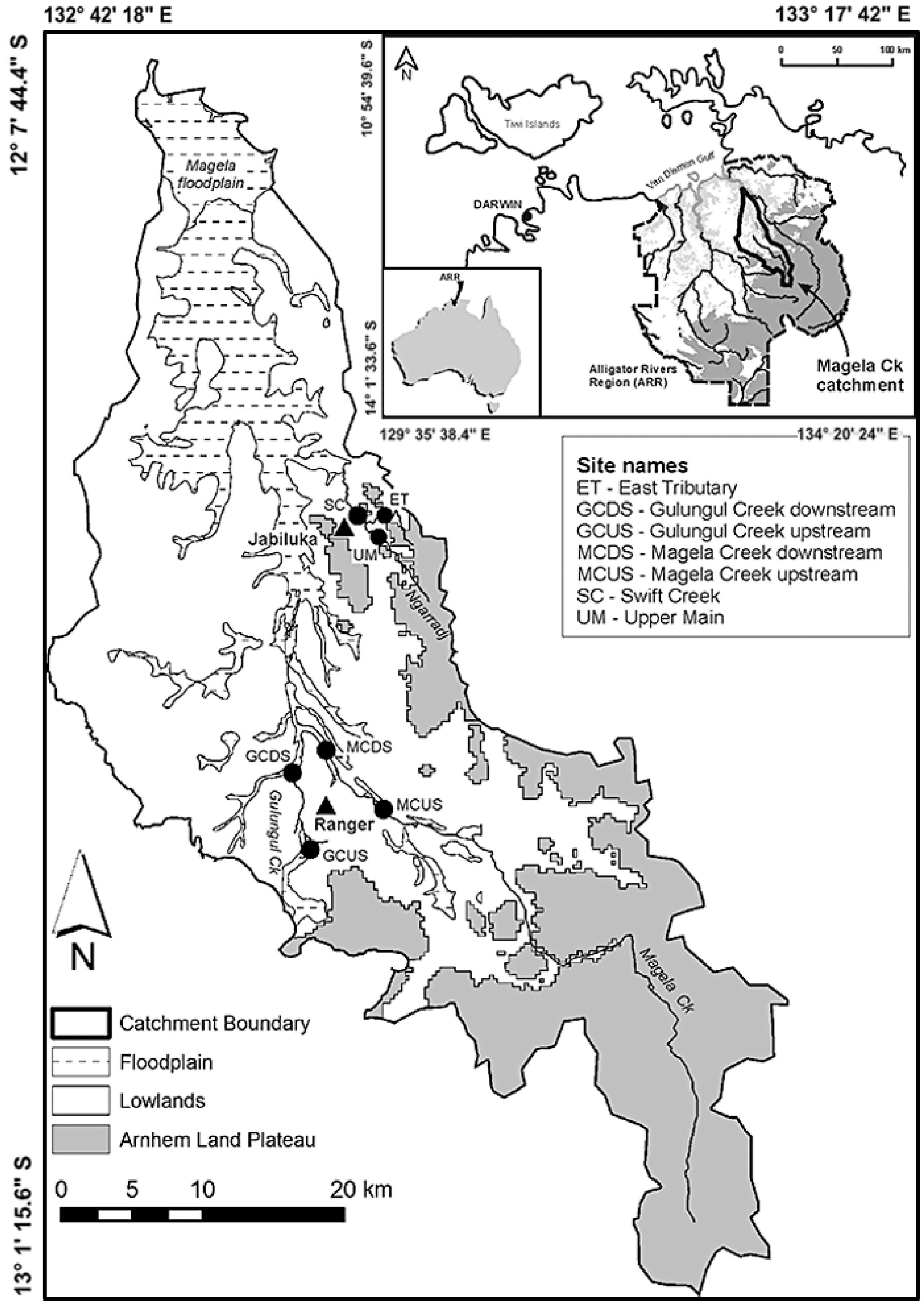
2. Site Description
The Ranger mine situated at coordinates 12°41′ S and 132°55′ E is an open-cut uranium mine that is operated by Energy Resources of Australia Ltd. (ERA) in the Northern Territory of Australia. The mine is positioned approximately 8 km to the east of Jabiru town and is contained within the 78 km
2 Ranger project area. While it is surrounded by the Kakadu National Park, the mine area is separate from the park itself (
Figure 1). Since 1981, it has been involved in the extraction of uranium oxide (U
3O
8) and is currently undergoing the process of rehabilitation and closure. Mining activities ceased in 2012, followed by the cessation of ore milling in early 2021, and the current focus is now on rehabilitation efforts [
5].
The geological context surrounding the Ranger mine primarily consists of mineralised metasediments and igneous rocks found within Pine Creek geosyncline, along with the younger sandstones of the Mamadawerre Formation. Geomorphically, the Ranger site is categorised as part of the extensively weathered Koolpinyah surface featuring plains, broad valleys, and low-gradient slopes, with isolated hills and ridges of resistant rock [
6]. As the mine is located in the monsoon tropics, it undergoes a distinct wet season spanning from October to April while the rest of the year is characterised by a dry season. Consequently, the streamflow exhibits significant seasonality. The average annual rainfall in the area amounts to 1557 mm [
7].
Figure 1.
Location of Ranger uranium mine, adapted from [
8] and reproduced under Creative Commons CC with attribution.
Figure 1.
Location of Ranger uranium mine, adapted from [
8] and reproduced under Creative Commons CC with attribution.
Due to its distinctive placement in the Northern Territory of Australia, with its proximity to the World Heritage-listed Kakadu National Park, as well as its location upstream of floodplains and wetlands designated as Wetlands of International Significance under the Ramsar Convention, the Ranger mine holds considerable environmental and cultural importance. The unique position necessitates careful consideration and sensitivity regarding the mine’s operations, as well as its forthcoming closure and rehabilitation processes. As a result, there has been growing emphasis on the formulation of suitable criteria for closure and the establishment of rehabilitation plans for the mine site [
8]. ERA is responsible for the rehabilitation of the Ranger mine based on laid out principles called environmental requirements (ERs). The supervising scientist has a supervisory role. As quoted in the environmental requirements, ERs pertaining to the erosion equilibrium of the landform require “erosion characteristics which, as far as can reasonably be achieved, do not vary significantly from those of comparable landforms in surrounding undisturbed areas”. Anticipated erosion rates are expected to be initially high, gradually approaching the natural rates over an extended period of time. Given the considerable length of these timeframes, the objective is to employ the most effective modelling techniques available to showcase that the erosion properties of the final landform will eventually be comparable to those of natural landscapes [
3].
The Ranger mine is adjacent to Magela Creek, a left-bank tributary of the East Alligator River [
5]. Gulungul Creek is a small tributary of Magela Creek that is adjacent to the tailings dam. It is one of the tributaries that would be the first to receive sediment generated from the mine site during and after rehabilitation [
9]. The Gulungul and Magela creeks are ephemeral sand bed braided streams which carry very large sand loads (bed and suspended bed) and small FSS (fine suspended sediment) loads. Environmental Research Institute of the Supervising Scientist (eriss) had monitoring sites in Gulungul Creek downstream (GCDS), Gulungul Creek upstream (GCUS), Magela Creek downstream (MCDS), and Magela Creek upstream (MCUS) of the mine (
Figure 2). The data obtained from eriss for this study were continuous discharge (m
3), and turbidity (NTU) and FSS (a <63 µm fraction of sediment samples collected in the auto-samplers; mg) data. Data were from August 2004 to August 2015 measured at a frequency of 6 min for Gulungul Creek GCDS and GCUS. Rainfall data for GCDS and GCUS in 10 min intervals were also obtained for modelling the Gulungul catchment in CAESAR-Lisflood [
3].
3. Landform Evolution Modelling
Numerical landscape evolution models (LEMs) are tools utilised for analysing geomorphic dynamics of landscapes. These models incorporate various factors such as pedogenesis, climate, geology, and vegetation growth. LEMs are capable of operating across a wide range of time scales spanning from years to millennia, and spatial scales encompassing sub-hectare areas to entire regions [
11]. Within the realm of predicting surface stability, models can be broadly classified into two categories: (1) soil loss prediction or soil erosion models; (2) topographic evolution models [
12].
Soil loss prediction or soil erosion models have typically been developed for agricultural purposes, but some of the soil loss prediction models that can be applied to mining landforms are RULSE, CREAMS, and WEPP [
13].
Topographic evolution models (TEM) or landscape evolution models (LEM) are process response models based on the modelling of erosion and accumulation of material over time across a landform. These models provide insights into the extended-term geomorphological changes experienced by a surface affected by erosion and deposition processes [
12]. They can also be used to forecast the emergence of drainage problem areas and gullies. Early models [
14] focussed on determining areas of aggradation (when more material entered an area than was removed) and areas of net erosion (where less material entered an area than was removed). However, with advancements in computing technology, this concept can now be applied to individual nodes on a digital terrain map (DTM). This advancement allows the generation of 3D graphic representations through recently developed models, enhancing the simulation capabilities.
SIBERIA is a sophisticated 3D TEM that offers the capability to simulate both runoff and erosion processes. It predicts the long-term evolution of channels and hillslopes in a catchment [
15]. The initial modelling of the Ranger mine focused on using SIBERIA and CAESAR LEMs to determine whether or not the uranium remaining in the waste rock would remain buried for 10,000 years. Extensive research efforts were dedicated to the development of landform evolution modelling (LEM) techniques in this context [
2]. This included field programs using plot and catchment studies to calibrate sediment transport and hydrology models for inputs to the SIBERIA LEM. The calibrated model was used to assess mine landform stability over a 1000 y period and the results were strengthened via comparison to catchment denudation rates and empirical modelling. Further field studies were conducted to assess the temporal change in SIBERIA parameter values as a landscape matures. The impact of extreme rainfall events on the Ranger landform was determined using CEASAR-Lisflood in the single-event mode. CAESAR-Lisflood has also been used for long-term (up to 10,000 y) erosion simulation on the Ranger landform to assess the effects of climate change through a comparison of the undisturbed Magela Creek catchment and the mine-disturbed catchment using simulations for both future rainfalls with and without a climate change factor applied [
2].
Until 2008, the SIBERIA LEM was the sole geomorphic computer modelling code employed to forecast the long-term behaviour of the rehabilitated landform at the Ranger mine. However, SIBERIA simulations relied on an average area–discharge relationship for a wet season as input without considering the time series hydrology of a single rainfall event or series of events. As a result, the average long-term erosion assessments conducted thus far did not explicitly account for the impact of an extreme rainfall event or a series of events comprising an ‘extreme’ wet season. To address this limitation, CAESAR [
16] was introduced as it incorporates slope processes (soil creep, and mass movement), hydrological processes, the multidirectional routing of river flow and fluvial erosion and deposition over a range of different grain sizes. CAESAR also features a tracing component that allows for the input of contaminant data to be used to evaluate downstream transport. This capability is particularly crucial as it enables the tracking of sediment lost from the landform through a river catchment, a functionality that is absent in SIBERIA. CAESAR-Lisflood LEM was utilised in this study as it works at a much finer temporal resolution compared to that of SIBERIA.
CAESAR-Lisflood LEM
CAESAR-Lisflood [
17,
18] combines a hydrologic model (TOPMODEL) and a hydraulic model (Lisflood) to simulate landscape development. It operates by routing water across a regular grid of cells and altering elevations of individual cells based on numerically calculated erosion and deposition rates resulting from fluvial and slope processes. Rainfall data are used to generate runoff over the landform using an adapted version of TOPMODEL [
19]. Surface flow is routed using Lisflood-FP [
20], a two-dimensional hydrodynamic flow model. Changes to landform morphology occur through the transport and deposition of sediments. The Einstein (1950) and Wilcock and Crowe (2003) sediment transport equations are the two options for calculating sediment transport in this version of the CAESAR-Lisflood model [
21,
22].
A significant feature of the CAESAR-Lisflood model is its ability to incorporate variable time interval rainfall data specific to the study area. This allows the modelling of the effects of specific rainfall events. As the climatic region in which the Ranger mine is situated is dominated by seasonal, high-intensity rainfall events, the capability to model specific rainfall events means that the CAESAR-Lisflood model is the most suitable choice for this study [
3].
CAESAR is capable of simulating the impact of extreme rainfall events by utilising time series data from actual or simulated rainfall events as input. This capability is particularly crucial considering the long duration for which the containment of radioactive material is required and the possibility of experiencing one or more very extreme rainfall events. Given the potential effects of climate change, there is an increased focus on testing the proposed design parameters for the constructed landform against extreme events, as the frequency of intense rainfall periods may potentially rise. because of. A digital elevation model of the landform, rainfall data, and particle size distribution data of the landform surface are the three key data inputs required in CAESAR-Lisflood. The presence or absence of a vegetation cover may also be incorporated into model simulations. The parameters for CAESAR-Lisflood used in this study are given in
Table 1. The particle size distribution (grain sizes and corresponding proportions) for the watershed is taken from Evans (2022) [
23]. Suspended sediment particle sizes are the mud and clay components (<63 µm fraction sediments) of the soil. There are three sediment transport equations available in CAESAR-Lisflood, namely Wilcock and Crow, Einstein and Mayer Peter Muller. The Wilcock and Crow sediment transport equation (Equation (1)) was used for modelling since it gave reasonable results comparable to the field data in this study. The transport potential of Wilcock and Crow [
22] formula is given by the following:
where, q
bk = fractional bed load sediment transport potential, u = bed shear velocity, W
k = transport function, R
k = ρ
sk/ρ
w − 1 = submerged specific gravity of grain class, ρ
sk = sediment grain density, ρ
w = water density, and g = gravitational constant [
22].
The fall velocity of suspended sediment is 0.026 m/s for 63 µm fraction sediments. Manning’s ‘n’ depicts the level of surface roughness affecting flow velocity and the flow path. The scaling factor ‘m’ in CAESAR-Lisflood controls the peak discharges and duration of a hydrograph generated by a rain event. Manning’s ‘n’ and ‘m’ values in the parameters are calibrated values. Descriptions of Manning’s n value selection are detailed in
Section 7. According to Bureau of Meteorology data, the average annual evaporation rate is 2000 mm in the Ranger mine area. Thus, the daily evaporation rate in the watershed is given as 0.0055 m/day [
24]. The maximum erosion limit of the catchment is given as 0.02 m for calibration and thus the active layer thickness which should be more than four times the maximum erosion limit is given as 0.1 m. The input/output difference is the minimum value of input for which the model gives its output. It is given as 0 m
3/s. All the other parameters in the model are taken as default values.
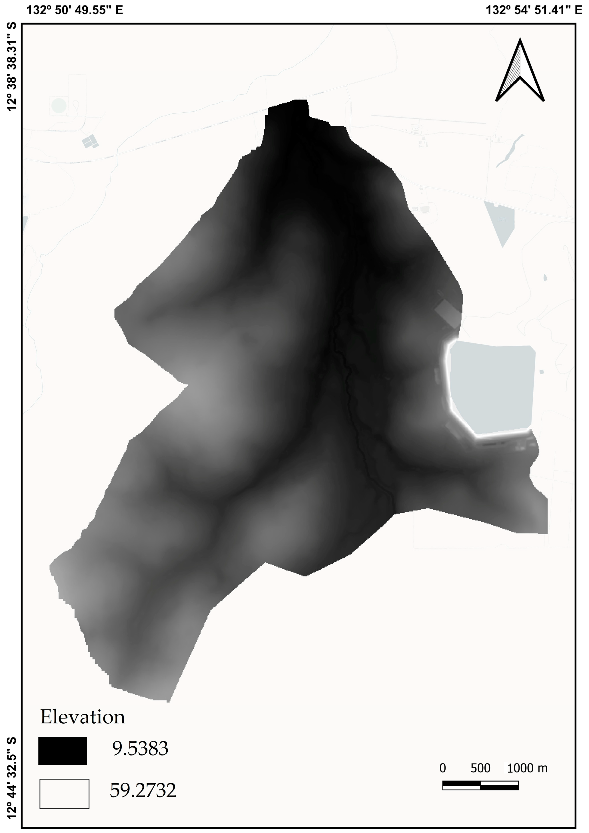
4. Catchment Digital Elevation Model
The DEM used in this study was a 10 m resolution digital elevation model of the Gulungul catchment obtained from eriss. The catchment area of 25 km
2 encompasses the Gulungul creek and parts of the Ranger mine with the waste rock dump and the trial landform (
Figure 3). The eriss monitoring sites at GCUS and GCDS record rainfall, discharge, and turbidity. These data were used for the calibration and validation of the model. Those that represented in gray color are waterbodies in
Figure 3,
Figure 4 and
Figure 5. The bigger one near the catchment being tailings dam.
5. Rainfall Data
The rainfall data input into CAESAR-Lisflood were hourly data from eriss. Rainfall data at 10 min intervals from 2005 to 2015 for GCUS and GCDS were obtained from eriss. There are two other BOM (Bureau of Meteorology) stations nearby the Gulungul catchment where rainfall data are available that would influence parts of the catchment. They are the Jabiru Airport and Jabiru Fire Station (
Figure 4). Half-hourly rainfall data for Jabiru airport/fire station were obtained from BOM from 2005 to 2015. The use of data from a number of gauging stations gave more accurate hourly discharge modelling results during hydrology calibration. Thus, four gauging station data were used in this study.
The model was initially calibrated for a rainfall event from 25 December 2011 to 28 December 2011. The event consisted of extreme hourly rainfall of 18 mm/h which is gives an EY (exceedance per year) of 12 for the area [
25]. This was a frequent event which had continuous rainfall, discharge and sediment data available and thus the event was used for calibration. The rainfall data of all four stations were converted into hourly rainfall intensity (mm) data for that time period, and the text file of the rainfall data was used as input in the hydrology tab of the model.
Voronoi polygons were drawn in the Quantum geographic information system (QGIS) [
26] for the four stations to determine the area of influence of each rainfall station, and these areas were clipped to the Gulungul catchment polygon as shown in
Figure 4. The catchment was divided into four sections where each of the station’s rainfall data were input. Thus, the Voronoi polygons in
Figure 4 depicted how the rainfall from four different rain gauges was spatially distributed in the catchment. The rasterised file of this DEM in *.ASC format was input into the hydroindex file in the hydrology tab of the model.
6. Input Discharge and Sediment
The input file was a text file with fourteen columns, where each row was one input time step (each time step was 1 h). The fourteen columns were time, discharge (m3s−1), three blank columns, and nine columns with the volumes of sediment being shown in m3 for each of the nine separate grain size fractions specified in the sediment tab of the model. The last column was the volume of fine suspended sediment (FSS).
The catchment input discharge (m3s−1) for Gulungul Creek at GCUS in 6 min intervals was obtained from eriss. Discharge data were averaged to obtain the hourly discharge at GCUS in m3s−1.
Turbidity can be used as a surrogate measure of observed FSS load [
27]. A site-specific relationship between FSS and turbidity for GCUS was developed for this study by Nair et al., 2021 [
2]. To estimate FSS, turbidity data (NTU) for Gulungul Creek at GCUS in 6 min intervals were obtained from eriss. The relationship indicated by Nair et al., 2021, was used to find the volume of FSS (m
3) load corresponding to hourly discharge (
Table A1). Volumes of sediment of the remaining eight separate grain sizes were required for the input text file. Since there were no available observed data for the bedload for each of these grain sizes during the calibration event period, bedload was quantified using a site-specific relationship between bedload and total sediment load.
The site specific relationship between total sediment load and bedload is as follows [
28]:
(r2 (coefficient of determination) = 0.99; p (probability value) < 0.001).
Particle size analysis data are available for GCUS during the period 2007–2008 from eriss. This gives the quantity of bedload sediment corresponding to respective grain sizes. Equation (2) can be used to find the total sediment load in one of the above data sets and the difference between total sediment load and bedload gives the total suspended load (total suspended sand + total suspended mud). The proportion of suspended sand to suspended mud for the catchment is 41:28 [
29]. Further data and calculations are shown in
Table A2 and
Table A3 in
Appendix A. Using the above data, the weight of the total sediment of each grain size was determined. The proportion of sediments of each grain size was thus determined and used to find the volume of sediments of separate grain sizes for the calibration rainfall event (
Table A4 in
Appendix A). The resulting text input file was entered into the reach input variable of the hydrology tab in the CAESAR-Lisflood model.
7. Manning’s n Values
Manning’s coefficient ‘n’ depicts the level of surface roughness affecting flow velocity and the flow path. Manning’s n [
30] is formulated as follows:
where v is average velocity in ms
−1, R is the hydraulic radius in m and s is the slope of the channel at the point of measurement. The chainage distances from the banks across the creek with the corresponding depth of the creek and velocity of flow data from eriss for Gulungul Creek were used to find Manning’s n using Equation (3). The slope of the channel was determined from DEM using GIS. The value was found to be around 0.06 across the stream. There are different areas on the Gulungul catchment based on vegetation and soil types depicting different roughness coefficients or Manning’s n values. The catchment polygon was divided into different polygons, namely waste rock, stream, riparian zone, swale and savanna woodlands (
Figure 5). This was mapped in GIS software using satellite imagery of the catchment. The shape file of the catchment and Manning’s polygon was overlapped, and the rasterised file was imported to the flow model tab of the CAESAR-Lisflood model. The stream was given an ‘n’ value of 0.06 and other areas were given values based on Chow (1959) [
31]. There are a range of values that could be used for each of the polygons divided based on their vegetation and soil types, and these values along with other parameters of the model were adjusted during calibration. The use of different Manning’s n values based on land cover and vegetation depicts a more realistic depiction of the watershed.
8. Results
8.1. Model Calibration
The Gulungul catchment was studied to return to background erosion levels in the 2011 wet season after the disturbance caused by trial landform construction in 2008 in the Ranger mine [
2]. Thus, a relatively large individual storm event in the 2011 wet season was selected for model calibration [
32]. The model was calibrated to observed hydrology and sediment output at GCDS for a rainfall event from 25 December 2011 to 28 December 2011. All the input data were sorted as described in the above sections and the model was run to obtain an output (catchment.dat) file. For a specified time, the output file contained fourteen columns: time, Qw (actual), Qw (expected), a blank column, and total sediment output in the time step (m
3), followed by nine columns that have the volumes in m
3 of sediment for each of the nine separate grain size fractions. The time interval for the output in this study was hourly (same as the input).
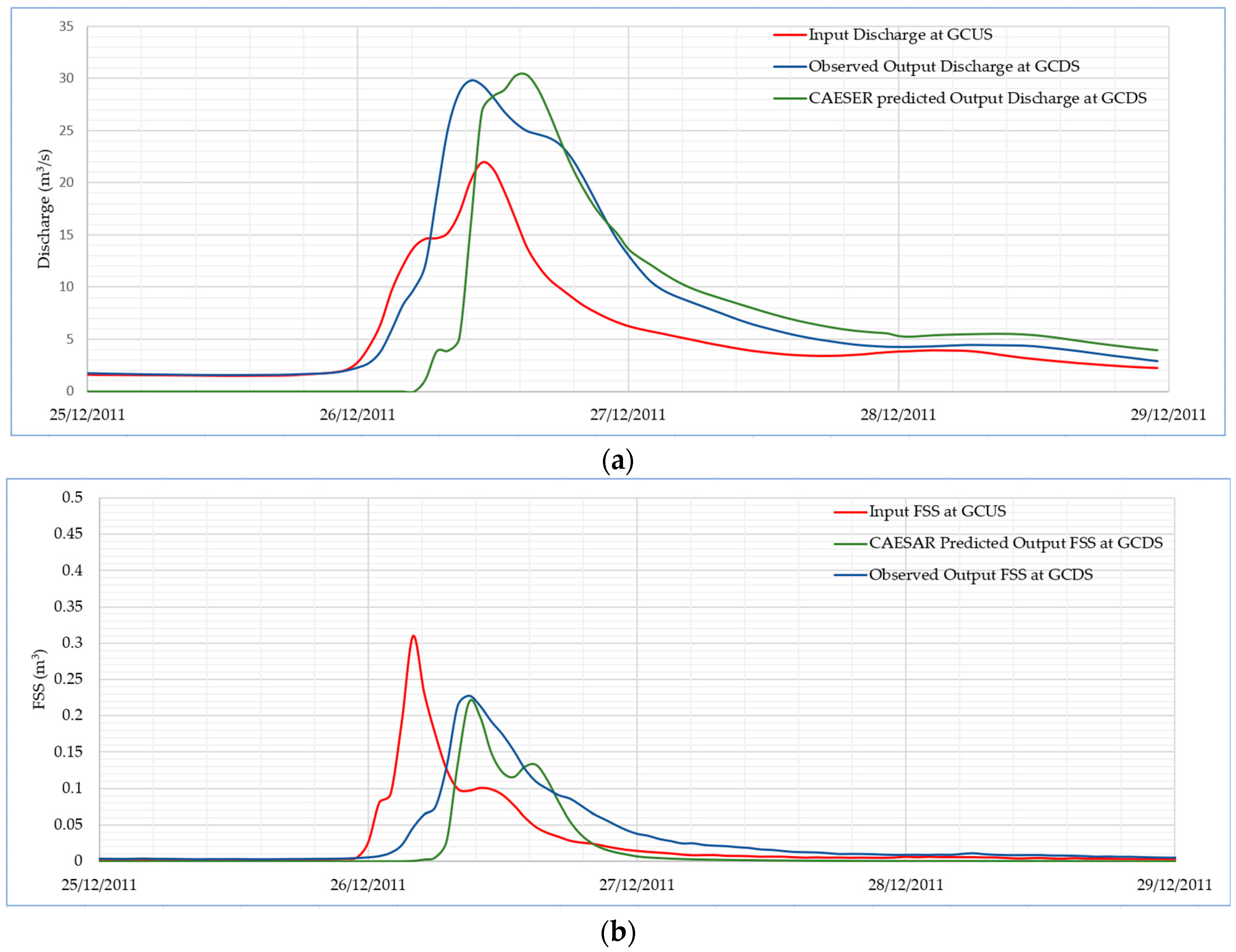
Modelled discharge and FSS data from the output file were compared with the observed data at GCDS. In the CAESAR-Lisflood model, the set of Manning’s coefficients, ‘n’ (level of surface roughness affecting flow velocity and flow path), and the hydrograph exponent ‘m’ (determines the peakiness and duration of the hydrograph) was adjusted so that the predicted discharge hydrograph and event FSS quantity were similar to the observed values. While calibrating, the best fit was determined by selecting the set of values for Manning’s ‘n’ and hydrograph exponent ‘m’ such that the modelled event FSS quantity was approximately same as the observed event FSS quantity and the modelled hydrology peak and duration were similar to the observed values as determined through visual assessment. The hydrology peak (
Figure 6a) and event sediment quantity were calibrated (
Figure 6b) with Manning’s n values of stream = 0.06, swale = 0.03, riparian zone = 0.07, savannah woodlands = 0.04 and waste rock = 0.02; hydrology exponent ‘m’ = 0.01. Total event FSS quantity for an event discharge was considered during the calibration of the model since the model was calibrated for future simulations to predict future FSS quantities during rainfall events [
2].
8.2. Model Validation
The model was run with calibrated parameters for a whole year encompassing the rainfall event used for calibration. Data for input discharge, rainfall at all four rainfall stations and sediment volume for different grain sizes were sorted for hourly input from 31 August 2010 to 31 August 2011. Since the model was run for a year, the rainfall initial loss (400 mm) and continuous loss (2.4 mm/h) were reduced from the total rainfall [
33]. The initial loss defines the volume of water that is required to fill the soil layer at the start of the simulation and continuous loss defines the rate at which precipitation will be infiltrated into the soil layer after the initial loss volume has been satisfied. In this study, there was no discharge contribution from rainfall until there was a cumulative rainfall of 400 mm; an hourly rainfall event of less than 2.4 mm/h was considered no rainfall and other events were reduced of 2.4 mm/h.
Model hydrology was validated since the CAESAR-Lisflood discharge output at GCDS was similar to the observed hydrology in terms of the peak and duration of the hydrograph (
Figure 7a) for the whole year. Regarding the sedigraph, the model simulated FSS spikes similar to those in the observed data at GCDS for the start of the wet season (
Figure 7b). Towards the end of wet season, CAESAR-Lisflood underpredicted the observed FSS spikes. The start of the wet season in 2011 on the Ranger mine site was estimated as 9 October 2011 and the end of the wet season was estimated as 9 April 2012 (Segura Pers. Comm.). The start and end of wet season were considered based on plant available water (PAW). The initial rise in PAW which was sustained was marked as the start of the wet season and the date after which PAW consistently declined was considered the end of the wet season. The reason behind the model underpredicting the event FSS quantity may have been due to change in vegetation ground cover and evapotranspiration towards the second half of the wet season. Ground cover vegetation is strongly seasonal with vigorous grass growth during the wet season and a substantial decline in grass foliage cover during the dry season. Most transpiration occurs from the grassy ground cover rather than from the trees, and ground cover transpiration is minimal at the start of the wet season but high during the middle to the end of the wet season [
34].
A quantitative comparison of the field-observed data and CAESAR-predicted data at GCDS for 2010–2011 is shown in
Figure 8 [
2]. The dark blue line is the best-fit line where the observed and predicted load are equal. The red dashed line is the 95% confidence limit and the blue dashed line is the 95% prediction limit of the best fit line. Event loads are shown as marker points in the graph. The red markers show CAESAR-Lisflood-predicted event loads corresponding to their observed loads in the early wet season. They are well within the prediction limits. The outlier marked in green is an event load on 8 February 2011 which is in the later part of the wet season. The quantitative comparison thus enforces that the fine suspended sediment value predicted in the early wet season is in accordance with that in the observed data. However, in the later part of wet season, CAESAR-Lisflood underpredicted data compared to the field-observed ones.
9. Conclusions
Calibrating and validating the model with variable input parameters gives an insight into how sensitive CAESAR-Lisflood is to each parameter. The model was run using different combinations of Manning’s ‘n’ and hydrology exponent ‘m’ to calibrate the hydrology and event sediment quantity to the observed values at the catchment output. While hydrology could be easily calibrated with ‘m’ = 0.01 and a range of Manning’s ‘n’ values over the catchment, sediment event output quantity narrowed the range of ‘n’ values that could be used to calibrate the model for the catchment. Using variable Manning’s n values over the catchment based on an ecological map based on soil type and vegetation community instead of a single value of n for the entire catchment is a more realistic depiction of the site scenario.
The sedigraph peak and event sediment quantity could not be calibrated together for the same values of Manning’s ‘n’. This may have been because the sediment values were computed from turbidity values using a linear equation relating to suspended sediment quantity and its corresponding turbidity. The equation was statistically generated with values taken over number of years and thus the equation represents an average situation where an individual event sediment peak may deviate from the actual. However, in this study the model was calibrated to th eobserved event sediment quantity since this value was required to check the landform stability for future simulations.
During validation, the Manning’s ‘n’ values that accurately calibrated event sediment quantity during the start of the wet season were inaccurate at the end of the season. From the second half of the wet season, a different set of Manning’s ‘n’ values were required for the accurate event sediment quantity calibration of the model. There were substantial changes in catchment vegetation and changes in soil properties (i.e., increased organic content) over the wet season. If the changing vegetation could be directly accounted for in the model, the validated model could be run for future simulations to determine event sediment quantity for a corresponding discharge and thus could be used to understand landscape equilibrium dynamics. This was one of the limitations of the model in this study.
Future work pertaining to the study should include the generation of long-term rainfall scenarios using climate records and global climate models. The modelled catchment along with long-term rainfall scenarios facilitates the prediction of discharge and sediment output for predicted wet and dry rainfall scenarios. This helps determine the dynamics of landform evolution of the catchment over the years post-mining.
Author Contributions
Conceptualisation: K.G.E. and D.N.; methodology: K.G.E. and D.N.; formal analysis: D.N.; writing—original draft preparation: D.N.; writing—review and editing: D.N., K.G.E. and S.B.; project administration: K.G.E. All authors have read and agreed to the published version of the manuscript.
Funding
This research received no external funding.
Data Availability Statement
Not applicable.
Acknowledgments
The Environmental Research Institute of the Supervising Scientist (eriss) is thanked for the provision of the data for this study. Professor Ken Evans’s time was provided by Surface Water & Erosion Solutions as an in-kind contribution.
Conflicts of Interest
The authors declare no conflict of interest.
Appendix A
Table A1.
Calculations to determine hourly FSS volume (m3) from observed turbidity data.
Table A1.
Calculations to determine hourly FSS volume (m3) from observed turbidity data.
Hourly Turbidity in NTU
(Observed Data) | Hourly Turbidity in mg/L (Using Turbidity–FSS Relationship) | Hourly Discharge in m3s−1 (Observed Data) | Hourly Discharge in L | Hourly Sediment Output in Mg (Hourly Discharge in L * Hourly Turbidity in mgL−1) | Hourly Sediment Output in Kg | Hourly Sediment Output in m3
(Density = 2650 kgm−3) |
|---|
| 2 | 1.04 | 1.569691 | 5,650,887.6 | 5,876,923.104 | 5.876923 | 0.002217707 |
| 2 | 1.04 | 1.55642 | 5,603,112 | 5,827,236.48 | 5.827236 | 0.002198957 |
| 1.94 | 1.0088 | 1.550194 | 5,580,698.4 | 5,629,808.546 | 5.629809 | 0.002124456 |
| 1.9 | 0.988 | 1.54398 | 5,558,328 | 5,491,628.064 | 5.491628 | 0.002072312 |
| 1.9 | 0.988 | 1.537784 | 5,536,022.4 | 5,469,590.131 | 5.46959 | 0.002063996 |
| 1.84 | 0.9568 | 1.527378 | 5,498,560.8 | 5,261,022.973 | 5.261023 | 0.001985292 |
| 1.83 | 0.9516 | 1.521929 | 5,478,944.4 | 5,213,763.491 | 5.213763 | 0.001967458 |
| 1.87 | 0.9724 | 1.51062 | 5,438,232 | 5,288,136.797 | 5.288137 | 0.001995523 |
| 1.76 | 0.9152 | 1.503162 | 5,411,383.2 | 4,952,497.905 | 4.952498 | 0.001868867 |
| 1.82 | 0.9464 | 1.495728 | 5,384,620.8 | 5,096,005.125 | 5.096005 | 0.001923021 |
| 1.85 | 0.962 | 1.484442 | 5,343,991.2 | 5,140,919.534 | 5.14092 | 0.00193997 |
| 1.87 | 0.9724 | 1.47205 | 5,299,380 | 5,153,117.112 | 5.153117 | 0.001944572 |
| 1.7 | 0.884 | 1.461762 | 5,262,343.2 | 4,651,911.389 | 4.651911 | 0.001755438 |
| 1.88 | 0.9776 | 1.460458 | 5,257,648.8 | 5,139,877.467 | 5.139877 | 0.001939576 |
| 1.77 | 0.9204 | 1.46515 | 5,274,540 | 4,854,686.616 | 4.854687 | 0.001831957 |
| 1.88 | 0.9776 | 1.469853 | 5,291,470.8 | 5,172,941.854 | 5.172942 | 0.001952054 |
| 2.06 | 1.0712 | 1.474563 | 5,308,426.8 | 5,686,386.788 | 5.686387 | 0.002145806 |
| 2.01 | 1.0452 | 1.479283 | 5,325,418.8 | 5,566,127.73 | 5.566128 | 0.002100426 |
| 1.83 | 0.9516 | 1.50433 | 5,415,588 | 5,153,473.541 | 5.153474 | 0.001944707 |
| 2.11 | 1.0972 | 1.569685 | 5,650,866 | 6,200,130.175 | 6.20013 | 0.002339672 |
| 2.22 | 1.1544 | 1.631615 | 5,873,814 | 6,780,730.882 | 6.780731 | 0.002558766 |
| 2.39 | 1.2428 | 1.70256 | 6,129,216 | 7,617,389.645 | 7.61739 | 0.002874487 |
| 2.54 | 1.3208 | 1.807704 | 6,507,734.4 | 8,595,415.596 | 8.595416 | 0.003243553 |
| 3.71 | 1.9292 | 2.055457 | 7,399,645.2 | 14,275,395.52 | 14.2754 | 0.005386942 |
| 13.26 | 6.8952 | 2.781294 | 10,012,658.4 | 69,039,282.2 | 69.03928 | 0.026052559 |
| 26.63 | 13.8476 | 4.291121 | 15,448,035.6 | 213,918,217.8 | 213.9182 | 0.080723856 |
| 20.42 | 10.6184 | 6.396291 | 23,026,647.6 | 244,506,154.9 | 244.5062 | 0.092266474 |
| 28.07 | 14.5964 | 9.66576 | 34,796,736 | 507,907,077.4 | 507.9071 | 0.191663048 |
| 36.36 | 18.9072 | 12.059806 | 43,415,301.6 | 820,861,790.4 | 820.8618 | 0.309759166 |
| 23.69 | 12.3188 | 13.835157 | 49,806,565.2 | 613,557,115.4 | 613.5571 | 0.231530987 |
| 16.85 | 8.762 | 14.624897 | 52,649,629.2 | 461,316,051.1 | 461.3161 | 0.174081529 |
| 12.16 | 6.3232 | 14.686552 | 52,871,587.2 | 334,317,620.2 | 334.3176 | 0.126157593 |
| 9.24 | 4.8048 | 15.209804 | 54,755,294.4 | 263,088,238.5 | 263.0882 | 0.099278581 |
| 8 | 4.16 | 17.119121 | 61,628,835.6 | 256,375,956.1 | 256.376 | 0.096745644 |
| 7.06 | 3.6712 | 20.183078 | 72,659,080.8 | 266,746,017.4 | 266.746 | 0.100658875 |
| 6.37 | 3.3124 | 21.950873 | 79,023,142.8 | 261,756,258.2 | 261.7563 | 0.098775946 |
| 6.03 | 3.1356 | 21.34665 | 76,847,940 | 240,964,400.7 | 240.9644 | 0.090929963 |
| 5.67 | 2.9484 | 19.185333 | 69,067,198.8 | 203,637,728.9 | 203.6377 | 0.076844426 |
| 5.15 | 2.678 | 16.512742 | 59,445,871.2 | 159,196,043.1 | 159.196 | 0.060073979 |
| 4.8 | 2.496 | 13.829853 | 49,787,470.8 | 124,269,527.1 | 124.2695 | 0.046894161 |
| 4.58 | 2.3816 | 12.049374 | 43,377,746.4 | 103,308,440.8 | 103.3084 | 0.038984317 |
| 4.46 | 2.3192 | 10.730926 | 38,631,333.6 | 89,593,788.89 | 89.59379 | 0.033808977 |
| 4.08 | 2.1216 | 9.847518 | 35,451,064.8 | 75,212,979.08 | 75.21298 | 0.028382256 |
| 4.05 | 2.106 | 9.021546 | 32,477,565.6 | 68,397,753.15 | 68.39775 | 0.025810473 |
| 4.18 | 2.1736 | 8.237199 | 29,653,916.4 | 64,455,752.69 | 64.45575 | 0.024322926 |
| 3.95 | 2.054 | 7.63155 | 27,473,580 | 56,430,733.32 | 56.43073 | 0.021294616 |
| 3.66 | 1.9032 | 7.079681 | 25,486,851.6 | 48,506,575.97 | 48.50658 | 0.018304368 |
| 3.4 | 1.768 | 6.622038 | 23,839,336.8 | 42,147,947.46 | 42.14795 | 0.015904886 |
| 3.25 | 1.69 | 6.245463 | 22,483,666.8 | 37,997,396.89 | 37.9974 | 0.01433864 |
| 3.08 | 1.6016 | 5.96578 | 21,476,808 | 34,397,255.69 | 34.39726 | 0.012980096 |
| 2.95 | 1.534 | 5.732923 | 20,638,522.8 | 31,659,493.98 | 31.65949 | 0.011946979 |
| 2.78 | 1.4456 | 5.521837 | 19,878,613.2 | 28,736,523.24 | 28.73652 | 0.010843971 |
| 2.5 | 1.3 | 5.292171 | 19,051,815.6 | 24,767,360.28 | 24.76736 | 0.009346174 |
| 2.33 | 1.2116 | 5.068929 | 18,248,144.4 | 22,109,451.76 | 22.10945 | 0.008343189 |
| 2.5 | 1.3 | 4.853902 | 17,474,047.2 | 22,716,261.36 | 22.71626 | 0.008572174 |
| 2.62 | 1.3624 | 4.614081 | 16,610,691.6 | 22,630,406.24 | 22.63041 | 0.008539776 |
| 2.41 | 1.2532 | 4.414846 | 15,893,445.6 | 19,917,666.03 | 19.91767 | 0.0075161 |
| 2.49 | 1.2948 | 4.214592 | 15,172,531.2 | 19,645,393.4 | 19.64539 | 0.007413356 |
| 2.49 | 1.2948 | 4.02859 | 14,502,924 | 18,778,386 | 18.77839 | 0.007086183 |
| 2.33 | 1.2116 | 3.85956 | 13,894,416 | 16,834,474.43 | 16.83447 | 0.006352632 |
| 2.47 | 1.2844 | 3.729177 | 13,425,037.2 | 17,243,117.78 | 17.24312 | 0.006506837 |
| 2.49 | 1.2948 | 3.616494 | 13,019,378.4 | 16,857,491.15 | 16.85749 | 0.006361317 |
| 2.24 | 1.1648 | 3.515267 | 12,654,961.2 | 14,740,498.81 | 14.7405 | 0.005562452 |
| 2.08 | 1.0816 | 3.443143 | 12,395,314.8 | 13,406,772.49 | 13.40677 | 0.005059159 |
| 2.25 | 1.17 | 3.395978 | 12,225,520.8 | 14,303,859.34 | 14.30386 | 0.005397683 |
| 2.12 | 1.1024 | 3.367167 | 12,121,801.2 | 13,363,073.64 | 13.36307 | 0.005042669 |
| 2.17 | 1.1284 | 3.376441 | 12,155,187.6 | 13,715,913.69 | 13.71591 | 0.005175816 |
| 2.03 | 1.0556 | 3.405045 | 12,258,162 | 12,939,715.81 | 12.93972 | 0.004882912 |
| 2.07 | 1.0764 | 3.467502 | 12,483,007.2 | 13,436,708.95 | 13.43671 | 0.005070456 |
| 1.97 | 1.0244 | 3.534771 | 12,725,175.6 | 13,035,669.88 | 13.03567 | 0.004919121 |
| 1.85 | 0.962 | 3.643486 | 13,116,549.6 | 12,618,120.72 | 12.61812 | 0.004761555 |
| 1.97 | 1.0244 | 3.727272 | 13,418,179.2 | 13,745,582.77 | 13.74558 | 0.005187012 |
| 2.33 | 1.2116 | 3.795791 | 13,664,847.6 | 16,556,329.35 | 16.55633 | 0.006247671 |
| 2.06 | 1.0712 | 3.824707 | 13,768,945.2 | 14,749,294.1 | 14.74929 | 0.005565771 |
| 2.26 | 1.1752 | 3.88128 | 13,972,608 | 16,420,608.92 | 16.42061 | 0.006196456 |
| 2.1 | 1.092 | 3.915546 | 14,095,965.6 | 15,392,794.44 | 15.39279 | 0.005808602 |
| 2.1 | 1.092 | 3.901942 | 14,046,991.2 | 15,339,314.39 | 15.33931 | 0.005788421 |
| 2.1 | 1.092 | 3.888367 | 13,998,121.2 | 15,285,948.35 | 15.28595 | 0.005768282 |
| 2.08 | 1.0816 | 3.863066 | 13,907,037.6 | 15,041,851.87 | 15.04185 | 0.005676171 |
| 2 | 1.04 | 3.774092 | 13,586,731.2 | 14,130,200.45 | 14.1302 | 0.005332151 |
| 2.06 | 1.0712 | 3.648362 | 13,134,103.2 | 14,069,251.35 | 14.06925 | 0.005309151 |
| 1.86 | 0.9672 | 3.479014 | 12,524,450.4 | 12,113,648.43 | 12.11365 | 0.004571188 |
| 1.64 | 0.8528 | 3.339059 | 12,020,612.4 | 10,251,178.25 | 10.25118 | 0.003868369 |
| 1.9 | 0.988 | 3.191403 | 11,489,050.8 | 11,351,182.19 | 11.35118 | 0.004283465 |
| 2.11 | 1.0972 | 3.080294 | 11,089,058.4 | 12,166,914.88 | 12.16691 | 0.004591289 |
| 1.86 | 0.9672 | 2.971337 | 10,696,813.2 | 10,345,957.73 | 10.34596 | 0.003904135 |
| 1.8 | 0.936 | 2.868075 | 10,325,070 | 9,664,265.52 | 9.664266 | 0.003646893 |
| 2.24 | 1.1648 | 2.775263 | 9,990,946.8 | 11,637,454.83 | 11.63745 | 0.004391492 |
| 1.98 | 1.0296 | 2.675196 | 9,630,705.6 | 9,915,774.486 | 9.915774 | 0.003741802 |
| 2.03 | 1.0556 | 2.596988 | 9,349,156.8 | 9,868,969.918 | 9.86897 | 0.00372414 |
| 1.99 | 1.0348 | 2.517013 | 9,061,246.8 | 9,376,578.189 | 9.376578 | 0.003538331 |
| 1.88 | 0.9776 | 2.438069 | 8,777,048.4 | 8,580,442.516 | 8.580443 | 0.003237903 |
| 1.9 | 0.988 | 2.368357 | 8,526,085.2 | 8,423,772.178 | 8.423772 | 0.003178782 |
| 1.9 | 0.988 | 2.303901 | 8,294,043.6 | 8,194,515.077 | 8.194515 | 0.00309227 |
| 1.9 | 0.988 | 2.255489 | 8,119,760.4 | 8,022,323.275 | 8.022323 | 0.003027292 |
| 1.9 | 0.988 | 2.208585 | 7,950,906 | 7,855,495.128 | 7.855495 | 0.002964338 |
Table A2.
Calculation of FSS volume pertaining to different grain sizes at GCDS.
Table A2.
Calculation of FSS volume pertaining to different grain sizes at GCDS.
| Particle Size (mm) | Mass in g
(Bedload) | Mass in g
(Total Sediment Load) | Cumulative Proportion | Absolute Proportion |
|---|
| 2 | | | 0.260 | 0.26 |
| 1.4 | 1.01 | 1.010 | 0.539 | 0.28 |
| 1 | 4.96 | 4.960 | 1.630 | 1.09 |
| 710 um | 25.46 | 25.460 | 7.292 | 5.66 |
| 500 um | 161.56 | 161.560 | 44.884 | 37.59 |
| 355 um | 195.14 | 195.140 | 54.158 | 9.27 |
| 250 um | 245.98 | 245.980 | 68.201 | 14.04 |
| 180 um | 252.43 | 252.430 | 69.982 | 1.78 |
| 125 um | 252.53 | 252.530 | 70.010 | 0.03 |
| 90 um | 252.54 | 252.540 | 70.013 | 0.00 |
| 63 um | 252.55 | 317.04 (252.55 + 64.49) | 87.829 | 17.82 |
| <63 um | 252.57 | 361.11 (252.57 + 44.045) | 100.000 | 12.17 |
Table A3.
Absolute proportions of sediments pertaining to corresponding particle sizes.
Table A3.
Absolute proportions of sediments pertaining to corresponding particle sizes.
Particle Size in m
(Input in CAESAR-Lisflood Is in m) | Absolute Proportions |
|---|
| 0.000063 | 12.17 |
| 0.000125 | 17.82 |
| 0.00025 | 1.81 |
| 0.0005 | 23.32 |
| 0.001 | 43.25 |
| 0.002 | 1.37 |
| 0.004 | 0.26 |
| 0.008 | 0 |
| 0.032 | 0 |
| Total sediment = 1.28 × Bedload1.02 = 1.28 × 252.571.02 = 361.1099 g |
| Suspended sand + suspended mud = 361.1099 − 252.57 = 108.54 g |
| Suspended sand: suspended mud = 41:28 |
| Suspended sand = 64.49478 g |
| Suspended mud = 44.04522 g |
Table A4.
Hourly input at GCUS—volume of sediments (m3) of corresponding grain sizes in m (shown in first row).
Table A4.
Hourly input at GCUS—volume of sediments (m3) of corresponding grain sizes in m (shown in first row).
| 0.032 | 0.008 | 0.004 | 0.002 | 0.001 | 0.0005 | 0.00025 | 0.000125 | 0.000063 |
|---|
| 0 | 0 | 4.74 × 10⁻⁵ | 0.0002497 | 0.007881333 | 0.00425 | 0.00033 | 0.003247291 | 0.002218 |
| 0 | 0 | 4.70 × 10⁻⁵ | 0.0002475 | 0.0078147 | 0.004214 | 0.000327 | 0.003219837 | 0.002199 |
| 0 | 0 | 4.54 × 10⁻⁵ | 0.0002392 | 0.007549936 | 0.004071 | 0.000316 | 0.003110748 | 0.002124 |
| 0 | 0 | 4.43 × 10⁻⁵ | 0.0002333 | 0.007364627 | 0.003971 | 0.000308 | 0.003034397 | 0.002072 |
| 0 | 0 | 4.41 × 10⁻⁵ | 0.0002323 | 0.007335073 | 0.003955 | 0.000307 | 0.00302222 | 0.002064 |
| 0 | 0 | 4.24 × 10⁻⁵ | 0.0002235 | 0.007055371 | 0.003804 | 0.000295 | 0.002906976 | 0.001985 |
| 0 | 0 | 4.20 × 10⁻⁵ | 0.0002215 | 0.006991993 | 0.00377 | 0.000293 | 0.002880863 | 0.001967 |
| 0 | 0 | 4.26 × 10⁻⁵ | 0.0002246 | 0.007091732 | 0.003824 | 0.000297 | 0.002921958 | 0.001996 |
| 0 | 0 | 3.99 × 10⁻⁵ | 0.0002104 | 0.006641619 | 0.003581 | 0.000278 | 0.002736501 | 0.001869 |
| 0 | 0 | 4.11 × 10⁻⁵ | 0.0002165 | 0.006834071 | 0.003685 | 0.000286 | 0.002815795 | 0.001923 |
| 0 | 0 | 4.14 × 10⁻⁵ | 0.0002184 | 0.006894305 | 0.003717 | 0.000289 | 0.002840613 | 0.00194 |
| 0 | 0 | 4.15 × 10⁻⁵ | 0.0002189 | 0.006910662 | 0.003726 | 0.000289 | 0.002847353 | 0.001945 |
| 0 | 0 | 3.75 × 10⁻⁵ | 0.0001976 | 0.006238513 | 0.003364 | 0.000261 | 0.002570412 | 0.001755 |
| 0 | 0 | 4.14 × 10⁻⁵ | 0.0002183 | 0.006892907 | 0.003717 | 0.000288 | 0.002840037 | 0.00194 |
| 0 | 0 | 3.91 × 10⁻⁵ | 0.0002062 | 0.006510448 | 0.00351 | 0.000272 | 0.002682455 | 0.001832 |
| 0 | 0 | 4.17 × 10⁻⁵ | 0.0002197 | 0.006937249 | 0.003741 | 0.00029 | 0.002858307 | 0.001952 |
| 0 | 0 | 4.58 × 10⁻⁵ | 0.0002416 | 0.007625811 | 0.004112 | 0.000319 | 0.003142011 | 0.002146 |
| 0 | 0 | 4.49 × 10⁻⁵ | 0.0002364 | 0.007464536 | 0.004025 | 0.000312 | 0.003075561 | 0.0021 |
| 0 | 0 | 4.15 × 10⁻⁵ | 0.0002189 | 0.00691114 | 0.003726 | 0.000289 | 0.00284755 | 0.001945 |
| 0 | 0 | 5.00 × 10⁻⁵ | 0.0002634 | 0.008314774 | 0.004483 | 0.000348 | 0.003425879 | 0.00234 |
| 0 | 0 | 5.47 × 10⁻⁵ | 0.000288 | 0.009093397 | 0.004903 | 0.000381 | 0.00374669 | 0.002559 |
| 0 | 0 | 6.14 × 10⁻⁵ | 0.0003236 | 0.010215411 | 0.005508 | 0.000428 | 0.004208985 | 0.002874 |
| 0 | 0 | 6.93 × 10⁻⁵ | 0.0003651 | 0.011527007 | 0.006215 | 0.000482 | 0.004749393 | 0.003244 |
| 0 | 0 | 0.0001151 | 0.0006064 | 0.019144226 | 0.010322 | 0.000801 | 0.007887864 | 0.005387 |
| 0 | 0 | 0.0005566 | 0.0029328 | 0.092586129 | 0.049922 | 0.003875 | 0.038147626 | 0.026053 |
| 0 | 0 | 0.0017246 | 0.0090872 | 0.286878123 | 0.154682 | 0.012006 | 0.11820042 | 0.080724 |
| 0 | 0 | 0.0019712 | 0.0103866 | 0.327898519 | 0.1768 | 0.013722 | 0.135101771 | 0.092266 |
| 0 | 0 | 0.0040947 | 0.0215759 | 0.68113614 | 0.367262 | 0.028505 | 0.280643839 | 0.191663 |
| 0 | 0 | 0.0066177 | 0.0348702 | 1.10082859 | 0.593557 | 0.046069 | 0.453566832 | 0.309759 |
| 0 | 0 | 0.0049464 | 0.0260639 | 0.822819654 | 0.443657 | 0.034435 | 0.339020722 | 0.231531 |
| 0 | 0 | 0.0037191 | 0.0195967 | 0.61865457 | 0.333573 | 0.025891 | 0.254899987 | 0.174082 |
| 0 | 0 | 0.0026952 | 0.0142018 | 0.448341485 | 0.241742 | 0.018763 | 0.184727058 | 0.126158 |
| 0 | 0 | 0.002121 | 0.011176 | 0.352818292 | 0.190236 | 0.014765 | 0.145369294 | 0.099279 |
| 0 | 0 | 0.0020669 | 0.0108908 | 0.343816688 | 0.185383 | 0.014389 | 0.141660425 | 0.096746 |
| 0 | 0 | 0.0021505 | 0.0113314 | 0.357723609 | 0.192881 | 0.014971 | 0.147390398 | 0.100659 |
| 0 | 0 | 0.0021103 | 0.0111194 | 0.35103202 | 0.189273 | 0.014691 | 0.144633309 | 0.098776 |
| 0 | 0 | 0.0019426 | 0.0102362 | 0.323148799 | 0.174239 | 0.013524 | 0.133144777 | 0.09093 |
| 0 | 0 | 0.0016417 | 0.0086505 | 0.273091325 | 0.147248 | 0.011429 | 0.11251994 | 0.076844 |
| 0 | 0 | 0.0012834 | 0.0067626 | 0.213492159 | 0.115113 | 0.008935 | 0.087963706 | 0.060074 |
| 0 | 0 | 0.0010018 | 0.005279 | 0.166653449 | 0.089858 | 0.006974 | 0.068665074 | 0.046894 |
| 0 | 0 | 0.0008329 | 0.0043885 | 0.13854328 | 0.074701 | 0.005798 | 0.057083035 | 0.038984 |
| 0 | 0 | 0.0007223 | 0.0038059 | 0.120151048 | 0.064784 | 0.005028 | 0.04950501 | 0.033809 |
| 0 | 0 | 0.0006064 | 0.003195 | 0.100865455 | 0.054386 | 0.004221 | 0.041558899 | 0.028382 |
| 0 | 0 | 0.0005514 | 0.0029055 | 0.091725797 | 0.049458 | 0.003839 | 0.037793149 | 0.02581 |
| 0 | 0 | 0.0005196 | 0.0027381 | 0.08643932 | 0.046607 | 0.003617 | 0.035614999 | 0.024323 |
| 0 | 0 | 0.0004549 | 0.0023972 | 0.075677252 | 0.040804 | 0.003167 | 0.031180778 | 0.021295 |
| 0 | 0 | 0.0003911 | 0.0020606 | 0.065050446 | 0.035075 | 0.002722 | 0.026802288 | 0.018304 |
| 0 | 0 | 0.0003398 | 0.0017904 | 0.056523115 | 0.030477 | 0.002365 | 0.02328883 | 0.015905 |
| 0 | 0 | 0.0003063 | 0.0016141 | 0.050956959 | 0.027476 | 0.002133 | 0.020995445 | 0.014339 |
| 0 | 0 | 0.0002773 | 0.0014612 | 0.046128938 | 0.024872 | 0.00193 | 0.019006189 | 0.01298 |
| 0 | 0 | 0.0002552 | 0.0013449 | 0.042457423 | 0.022893 | 0.001777 | 0.01749344 | 0.011947 |
| 0 | 0 | 0.0002317 | 0.0012207 | 0.038537531 | 0.020779 | 0.001613 | 0.015878354 | 0.010844 |
| 0 | 0 | 0.0001997 | 0.0010521 | 0.033214627 | 0.017909 | 0.00139 | 0.013685194 | 0.009346 |
| 0 | 0 | 0.0001782 | 0.0009392 | 0.0296502 | 0.015987 | 0.001241 | 0.012216568 | 0.008343 |
| 0 | 0 | 0.0001831 | 0.000965 | 0.030463971 | 0.016426 | 0.001275 | 0.012551861 | 0.008572 |
| 0 | 0 | 0.0001824 | 0.0009613 | 0.030348834 | 0.016364 | 0.00127 | 0.012504421 | 0.00854 |
| 0 | 0 | 0.0001606 | 0.0008461 | 0.026710874 | 0.014402 | 0.001118 | 0.011005498 | 0.007516 |
| 0 | 0 | 0.0001584 | 0.0008345 | 0.026345739 | 0.014205 | 0.001103 | 0.010855054 | 0.007413 |
| 0 | 0 | 0.0001514 | 0.0007977 | 0.025183026 | 0.013578 | 0.001054 | 0.010375989 | 0.007086 |
| 0 | 0 | 0.0001357 | 0.0007151 | 0.022576116 | 0.012173 | 0.000945 | 0.009301882 | 0.006353 |
| 0 | 0 | 0.000139 | 0.0007325 | 0.023124133 | 0.012468 | 0.000968 | 0.009527677 | 0.006507 |
| 0 | 0 | 0.0001359 | 0.0007161 | 0.022606983 | 0.012189 | 0.000946 | 0.0093146 | 0.006361 |
| 0 | 0 | 0.0001188 | 0.0006262 | 0.019767959 | 0.010659 | 0.000827 | 0.008144856 | 0.005562 |
| 0 | 0 | 0.0001081 | 0.0005695 | 0.017979346 | 0.009694 | 0.000752 | 0.007407906 | 0.005059 |
| 0 | 0 | 0.0001153 | 0.0006076 | 0.019182398 | 0.010343 | 0.000803 | 0.007903591 | 0.005398 |
| 0 | 0 | 0.0001077 | 0.0005677 | 0.017920743 | 0.009663 | 0.00075 | 0.007383761 | 0.005043 |
| 0 | 0 | 0.0001106 | 0.0005827 | 0.018393925 | 0.009918 | 0.00077 | 0.007578722 | 0.005176 |
| 0 | 0 | 0.0001043 | 0.0005497 | 0.017352993 | 0.009357 | 0.000726 | 0.007149834 | 0.004883 |
| 0 | 0 | 0.0001083 | 0.0005708 | 0.018019493 | 0.009716 | 0.000754 | 0.007424448 | 0.00507 |
| 0 | 0 | 0.0001051 | 0.0005538 | 0.017481674 | 0.009426 | 0.000732 | 0.007202854 | 0.004919 |
| 0 | 0 | 0.0001017 | 0.000536 | 0.016921713 | 0.009124 | 0.000708 | 0.006972137 | 0.004762 |
| 0 | 0 | 0.0001108 | 0.0005839 | 0.018433713 | 0.009939 | 0.000771 | 0.007595116 | 0.005187 |
| 0 | 0 | 0.0001335 | 0.0007033 | 0.022203105 | 0.011972 | 0.000929 | 0.009148193 | 0.006248 |
| 0 | 0 | 0.0001189 | 0.0006265 | 0.019779754 | 0.010665 | 0.000828 | 0.008149716 | 0.005566 |
| 0 | 0 | 0.0001324 | 0.0006975 | 0.022021095 | 0.011874 | 0.000922 | 0.0090732 | 0.006196 |
| 0 | 0 | 0.0001241 | 0.0006539 | 0.02064273 | 0.01113 | 0.000864 | 0.008505282 | 0.005809 |
| 0 | 0 | 0.0001237 | 0.0006516 | 0.02057101 | 0.011092 | 0.000861 | 0.008475732 | 0.005788 |
| 0 | 0 | 0.0001232 | 0.0006493 | 0.020499442 | 0.011053 | 0.000858 | 0.008446244 | 0.005768 |
| 0 | 0 | 0.0001213 | 0.000639 | 0.020172093 | 0.010877 | 0.000844 | 0.008311369 | 0.005676 |
| 0 | 0 | 0.0001139 | 0.0006003 | 0.01894951 | 0.010217 | 0.000793 | 0.007807636 | 0.005332 |
| 0 | 0 | 0.0001134 | 0.0005977 | 0.018867773 | 0.010173 | 0.00079 | 0.007773959 | 0.005309 |
| 0 | 0 | 9.77 × 10⁻⁵ | 0.0005146 | 0.016245184 | 0.008759 | 0.00068 | 0.006693391 | 0.004571 |
| 0 | 0 | 8.26 × 10⁻⁵ | 0.0004355 | 0.013747491 | 0.007413 | 0.000575 | 0.005664284 | 0.003868 |
| 0 | 0 | 9.15 × 10⁻⁵ | 0.0004822 | 0.015222667 | 0.008208 | 0.000637 | 0.006272091 | 0.004283 |
| 0 | 0 | 9.81 × 10⁻⁵ | 0.0005169 | 0.016316617 | 0.008798 | 0.000683 | 0.006722824 | 0.004591 |
| 0 | 0 | 8.34 × 10⁻⁵ | 0.0004395 | 0.013874596 | 0.007481 | 0.000581 | 0.005716655 | 0.003904 |
| 0 | 0 | 7.79 × 10⁻⁵ | 0.0004105 | 0.012960403 | 0.006988 | 0.000542 | 0.005339986 | 0.003647 |
| 0 | 0 | 9.38 × 10⁻⁵ | 0.0004944 | 0.015606577 | 0.008415 | 0.000653 | 0.006430271 | 0.004391 |
| 0 | 0 | 7.99 × 10⁻⁵ | 0.0004212 | 0.013297693 | 0.00717 | 0.000557 | 0.005478957 | 0.003742 |
| 0 | 0 | 7.96 × 10⁻⁵ | 0.0004192 | 0.013234925 | 0.007136 | 0.000554 | 0.005453095 | 0.003724 |
| 0 | 0 | 7.56 × 10⁻⁵ | 0.0003983 | 0.012574596 | 0.00678 | 0.000526 | 0.005181024 | 0.003538 |
| 0 | 0 | 6.92 × 10⁻⁵ | 0.0003645 | 0.011506927 | 0.006204 | 0.000482 | 0.00474112 | 0.003238 |
| 0 | 0 | 6.79 × 10⁻⁵ | 0.0003578 | 0.011296822 | 0.006091 | 0.000473 | 0.004654552 | 0.003179 |
| 0 | 0 | 6.61 × 10⁻⁵ | 0.0003481 | 0.010989373 | 0.005925 | 0.00046 | 0.004527876 | 0.003092 |
| 0 | 0 | 6.47 × 10⁻⁵ | 0.0003408 | 0.010758453 | 0.005801 | 0.00045 | 0.004432731 | 0.003027 |
| 0 | 0 | 6.33 × 10⁻⁵ | 0.0003337 | 0.010534725 | 0.00568 | 0.000441 | 0.00434055 | 0.002964 |
References
- Hancock, G.; Verdon-Kidd, D.; Lowry, J. Sediment output from a post-mining catchment–Centennial impacts using stochastically generated rainfall. J. Hydrol. 2017, 544, 180–194. [Google Scholar] [CrossRef]
- Nair, D.; Evans, K.G.; Bellairs, S.; Narayan, M.R. Stream Suspended Mud as an Indicator of Post-Mining Landform Stability in Tropical Northern Australia. Water 2021, 13, 3172. [Google Scholar] [CrossRef]
- Nair, D.; Bellairs, S.M.; Evans, K. An approach to simulate long-term erosion equilibrium of a rehabilitated mine landform. In Proceedings of the Mine Closure 2022: 15th International Conference on Mine Closure, Brisbane, QLD, Australia, 4–6 October 2022; Tibbett, M., Fourie, A.B., Boggs, G., Eds.; Australian Centre for Geomechanics: Brisbane, QLD, Australia, 2022; pp. 1063–1074. [Google Scholar]
- Lowry, J.B.C.; Coulthard, T.J.; Hancock, G.R.; Jones, D.R. Assessing soil erosion on a rehabilitated landform using the CAESAR landscape evolution model. In Proceedings of the Mine Closure 2011: Sixth International Conference on Mine Closure, Lake Louise, AB, Canada, 18–21 September 2011; Tibbett, M., Fourie, A.B., Beersing, G., Eds.; Australian Centre for Geomechanics: Perth, WA, Australia, 2011; pp. 613–621. [Google Scholar]
- Australian Government. Closure and Rehabilitation Process of the Ranger Uranium Mine. Australian Government. Department of Agriculture, Water and Environment. 2020. Available online: https://www.environment.gov.au/science/supervising-scientist/ranger-mine/closure-rehabilitation (accessed on 20 October 2022).
- East, T.J. Landform evolution. In Landscape and Vegetation Ecology of the Kakadu Region, Northern Australia; Finlayson, C.M., Oertzen, I., Eds.; Springer: Berlin/Heidelberg, Germany, 1996; pp. 37–55. [Google Scholar]
- Bureau of Meteorology. Annual Climate Statement 2019; Australian Government: Canberra, ACT, Australia, 2020. [Google Scholar]
- Lowry, J.; Narayan, M.; Hancock, G.; Evans, K. Understanding post-mining landforms: Utilising pre-mine geomorphology to improve rehabilitation outcomes. Geomorphology 2019, 328, 93–107. [Google Scholar] [CrossRef]
- Erskine, W.; Saynor, M. Assessment of the Off-Site Geomorphic Impacts of Uranium Mining on Magela Creek, Northern Territory, Australia; Supervising Scientist Report 156, Supervising Scientist, Darwin; Department of Environment, Australian Government: Canberra, ACT, Australia, 2000. [Google Scholar]
- Moliere, D.R.; Evans, K.G. Development of trigger levels to assess catchment disturbance on stream suspended sediment loads in the Magela Creek catchment, Northern Territory, Australia. Geogr. Res. 2010, 48, 370–385. [Google Scholar] [CrossRef]
- Tucker, G.E.; Hancock, G.R. Modelling landscape evolution. Earth Surf. Process. Landf. 2010, 35, 28–50. [Google Scholar] [CrossRef]
- Evans, K.; Aspinall, T.; Bell, L. Erosion prediction models and factors affecting the application of the Universal Soil Loss Equation to post-mining landscapes in Central Queensland. In Proceedings of the Queensland Coal Symposium, Brisbane, QLD, Australia, 29–30 August 1991. [Google Scholar]
- Evans, K.G. Determination of Interrill Erodibility Parameters for Selected Overburden Spoil Types from Central Queensland Open-Cut Coal Mines; University of Queensland: Brisbane, QLD, Australia, 1992. [Google Scholar]
- Kirkby, M. Hillslope process-response models based on the continuity equation. Inst. Br. Geogr. Ser. Publ. 1971, 3, 5–30. [Google Scholar]
- Willgoose, G.; Bras, R.; Rodriguez-Iturbe, I. Modelling of the Erosional Impacts of Landuse Change: A New Approach Using a Physically Based Catchment Evolution Model. In Hydrology and Water Resources Symposium 1989: Comparisons in Austral Hydrology; Preprints of Papers; Institution of Engineers: Canberra, NSW, Australia, 1989. [Google Scholar]
- Coulthard, T.J. Landscape evolution models: A software review. Hydrol. Process. 2001, 15, 165–173. [Google Scholar] [CrossRef]
- Coulthard, T. Simulating upland river catchment and alluvial fan evolution. Earth Surf. Process. Landf. 2002, 27, 269–288. [Google Scholar] [CrossRef]
- Coulthard, T.; Kirkby, M.; Macklin, M. Modelling geomorphic response to environmental change in an upland catchment. Hydrol. Process. 2000, 14, 2031–2045. [Google Scholar] [CrossRef]
- Beven, K.J.; Kirkby, M.J. A physically based, variable contributing area model of basin hydrology/Un modèle à base physique de zone d’appel variable de l’hydrologie du bassin versant. Hydrol. Sci. J. 1979, 24, 43–69. [Google Scholar] [CrossRef] [Green Version]
- Bates, P.D.; Horritt, M.S.; Fewtrell, T.J. A simple inertial formulation of the shallow water equations for efficient two-dimensional flood inundation modelling. J. Hydrol. 2010, 387, 33–45. [Google Scholar] [CrossRef]
- Einstein, H.A. The Bed-Load Function for Sediment Transportation in Open Channel Flows; US Government Printing Office: Washington, DC, USA, 1950.
- Wilcock, P.R.; Crowe, J.C. Surface-based transport model for mixed-size sediment. J. Hydraul. Eng. 2003, 129, 120–128. [Google Scholar] [CrossRef]
- Evans, K. Assessment of broader catchment surface water impacts of redevelopment of the Rustler’s Roost mine and Quest 19 mining precinct.Volume 3. Preprints.org 2023, 2023061072. [Google Scholar]
- Bureau of Meteorology. Evaporation: Average Monthly & Annual Evaporation. 2006. Available online: http://www.bom.gov.au/watl/evaporation/ (accessed on 13 June 2023).
- Bureau of Meteorology. Design Rainfall Data System (2016), Australian Government. 2016. Available online: http://www.bom.gov.au/water/designRainfalls/revised-ifd (accessed on 20 September 2022).
- QGIS Development Team. QGIS Geographic Information System. Open Source Geospatial Foundation Project. 2022. Available online: https://qgis.osgeo.org (accessed on 16 September 2022).
- Moliere, D.; Saynor, M.; Evans, K. Suspended sediment concentration-turbidity relationships for Ngarradj—A seasonal stream in the wet-dry tropics. Australas. J. Water Resour. 2005, 9, 37–48. [Google Scholar] [CrossRef]
- Saynor, M.J.; Evans, K.G. Sediment loss from a waste rock dump, ERA Ranger Mine, Northern Australia. Aust. Geogr. Stud. 2001, 39, 34–51. [Google Scholar] [CrossRef]
- Evans, K.; Moliere, D.R.; Saynor, M.J.; Erskine, W.D.; Bellio, M. Baseline suspended-sediment, solute, EC and turbidity characteristics for the Ngarradj catchment, Northern Territory, and the impact of mine construction. Superv. Sci. Rep. 2004, 1–75. [Google Scholar]
- Manning, R. On the flow of water in open channels and pipes. Trans. Inst. Civ. Eng. Irel. 1891, 20. [Google Scholar]
- Chow, V.T. Open-Channel Hydraulics; The Blackburn Press: Caldwell, NJ, USA, 1959. [Google Scholar]
- Bureau of Meteorology, A.G. Northern Territory in February 2011: Darwin Airport Smashes Rainfall Records. 2011. Available online: http://www.bom.gov.au/climate/current/month/nt/archive/201102.summary.shtml (accessed on 17 June 2021).
- EnviroConsult Australia Pty Ltd. Existing Hydrological Condition and Hydrology Model Calibration; Grants Lithium Project EIS; EnviroConsult Australia Pty Ltd.: Darwin, NT, Australia, 2018; p. 59. [Google Scholar]
- Hutley, L.; O’grady, A.; Eamus, D. Evapotranspiration from Eucalypt open-forest savanna of Northern Australia. Funct. Ecol. 2000, 14, 183–194. [Google Scholar] [CrossRef]
| Disclaimer/Publisher’s Note: The statements, opinions and data contained in all publications are solely those of the individual author(s) and contributor(s) and not of MDPI and/or the editor(s). MDPI and/or the editor(s) disclaim responsibility for any injury to people or property resulting from any ideas, methods, instructions or products referred to in the content. |
© 2023 by the authors. Licensee MDPI, Basel, Switzerland. This article is an open access article distributed under the terms and conditions of the Creative Commons Attribution (CC BY) license (https://creativecommons.org/licenses/by/4.0/).


