An Open-Source, Low-Cost Apparatus for Conductivity Measurements Based on Arduino and Coupled to a Handmade Cell

Abstract

Electrical conductivity is one of the main parameters for the characterization of water solutions and for the monitoring of water sources. In this paper, we describe a very inexpensive prototype for conductivity measurements based on Arduino UNO R3 coupled to an open-source circuit board with only passive components. We designed the printed circuit board (PCB) and the suitable handmade cell using stainless-steel electrodes and wrote the freeware management software; the assembly of the prototype, including a temperature probe, and results were relatively simple. In order to allow for replicates, the instrument design, schematics, and software are available with an open-source license. Thirty-one bottles of spring waters with conductivities of between 15.2 and 2000 µS cm⁻¹ were tested using both this prototype and a commercial conductivity meter. Data correlation produced an equation that allowed us to obtain the conductivity value, starting with the value furnished by the Arduino apparatus in arbitrary units. The prototype is accurate enough (inaccuracy lower than 6% excluding very low conductivity values) and precise (RSD% of about 5%). Even if a lot of commercial instruments for conductivity are available, we propose a prototype built with the aim of lowering the cost of measurements, while ensuring that they remain useful for lab or in situ application, as well as for continuous water monitoring/management systems. A further aim was to propose the building of the instrument as a laboratory exercise; this can help students to better understand basic theoretical concepts regarding conductivity, electronic components, and the acquisition and treatment of analytical data.

1. Introduction

The first scientific studies on conductivity measurements date back to the mid-1800s, and even today, these are widely used as indicators in many analytical contexts [1,2,3,4,5]. The measurement of conductivity—that is, the ability to conduct electrical current—is used to characterize water samples [6] because of its correlation with the total salt content of water solutions. Conductivity is also dependent on the ions’ mobility, which, in turn, depends on their mass/charge ratio. The abovementioned correlation is not perfect, but even if the measurement results are neither qualitative nor quantitative, the parameter remains fundamental as an alternative to very expensive analyses such as ion chromatography, atomic absorption spectroscopy, or inductively coupled plasma mass spectrometry [7]. For instance, in some cases, if low conductivity is measured, further expensive qualitative and quantitative analyses can be avoided.

The total soluble salt content determines the salinity of a solution, which is an essential parameter to be tested for the evaluation of the water quality and, in turn, determines what its use can be.

As an example, the measurement of conductivity as an index of salinity is essential in the agri-food sector, such as, in hydroponic and aeroponic cultures, regarding plant irrigation; an economic and versatile conductivity meter with good strength/endurance in an adverse environment that does not require too-frequent maintenance and controlling could be very useful [8,9,10,11,12].

The conductivity measurement becomes more and more essential considering the increasing global crisis of freshwater resources, which involves the need to monitor freshwater extracted from groundwater [13].

In a completely different sector, the cultural heritage field, conductivity and ion chromatographic analyses are used for the determination of the salt content of stone materials, which is one of the main causes of stone degradation. Nevertheless, the more expensive and time-consuming chromatography method can also be avoided in this case, especially for samples with low conductivity [14].

In many applications, continuous monitoring of conductivity is required; the use of computers to monitor environment parameters with the aid of self-designed software, for example, in agriculture, dates back to the early 1980s. Today, these systems can be developed with microcontrollers such as Arduino, Raspberry Pi, or BeagleBone [15,16,17].

Surely, such a smart monitoring system will lower the price of the control system [18].

A lot of projects based on Arduino are also available online, but, unfortunately, very few of them are correct from an analytical point of view, because the ease of finding ready-to-use “sensors” at very small prices allows non-experts to propose instruments that probably have poor accuracy, or do not work at all. In this paper, a prototype and a protocol for water conductivity measures is proposed that, at the same time, is simple and can further lower costs as it is based on an Arduino apparatus, a shield, and a hand-made electrode. The proposed open source allows anyone with high-school skills to reproduce and calibrate the apparatus, which can be built at a price of EUR 10–15. The low cost allows for the possibility of setting up a laboratory exercise for students, covering different topics such as electrochemistry, basic electronic components, microcontroller programming, and data treatment [19,20,21]. The proposed prototype can be easily used both in lab and in situ, even in environments where it could be stolen, as this would cause minimal economic damage. The prototype requires a PC, but we are working to add a memory card and a battery.

All Supplementary Materials (SM) can be downloaded by following link at the end of this paper.

Arduino Uno is a board used to develop microprocessor-based projects. It was created in Ivrea (the city of the historic former Olivetti) by a company of the Telecom group, and the first one appeared in 2005 (thanks must be given to the inventors, listed in Figure S1 of the Supplementary Materials). The board, which is hardly any bigger than a credit card, consists of a printed circuit board (PCB) and some integrated circuit (IC) to support an Atmel microcontroller (µC). The peculiarity of the Arduino is not in the microcontroller—whose 8-bit series was created in the 1990s with none of the speed present in an AMD/Intel modern CPU—but in the development software, an open-source integrated development environment (IDE), which hides the complexity of programming a microcontroller to newcomers, presenting instead a “simple” C language, with the compiler able to produce a “machine code” to be upload inside the µC for near-real-time processing.

Arduino boards can be used for measuring whichever parameter (e.g., light, temperature, pressure, sound, digital signal, and more) for which purpose the electronic sensor exists. For this reason, it has recently been widely used by the scientific community for the development of new, open-source, inexpensive devices [22]. For instance, some of these commercial devices allow for the detection of atmospheric particulate matter (PM) or phosphorus in polluted waters. In addition, they have been used to build a data acquisition system for chemical instrumentation, to drive an LED system for microalgae cultivation, and to measure multiple parameters in water matrices [23,24,25,26]. Some reviews on the use of Arduino as in-lab measurement devices are available in the literature [27].

The first conductivity measurement approach using the Arduino was proposed for ocean water, to which parallel-finger electrodes already present on the market were connected [28]. In 1953, L.G. Smith proposed a circuit for the calibration of conductivity meters, the first seeking to standardize the measurement of conductivity, and though it now uses direct current [29], it is still used today; the authors of this paper had the idea of modifying it by coupling it with an Arduino board and a hand-made conductivity cell to obtain an inexpensive sensor that would preserve and maintain the peculiarities of an analytically correct conductivity measurement.

Further, instead of employing expensive interfaces (shields) to be used as a bridge between Arduino and our hand-made or commercial cell, we propose a self-made, open-source circuit, so that, except for the Arduino board, the entire apparatus can be made by hand (Figure 1), starting, as already said, by modifying the circuit proposed by Smith (Figure 2).

It can be seen that, to build this cell, as well as the whole apparatus, inexpensive materials were used. Despite this, a sensitivity no lower than that of several commercial more expensive instruments was obtained. A further cost reduction comes from the use of an open-source circuit, also made using inexpensive materials. Of course, similarly to all commercial instruments, this prototype requires calibration.

Our aim was, therefore, to create an inexpensive apparatus with the same peculiarities of a commercial instrument for analytically correct conductivity measurement. Of course, the user can buy an interface/module to connect a commercial conductivity cell to Arduino, but the apparatus would be expensive and would not fulfil the didactic aim of this project. The conductivity cell and the circuit have been optimized for measures in a conductivity range starting from very low values (2 or 3 µS, the level needed to control the quality of distilled water), up to 2000 µS, the level required for a spring source, countryside well, or historical fountain. Measures performed directly “in situ” as well as monitoring measures can be also performed to build an environment water quality monitoring system based on Arduino [30]. Another important objective is the use of our prototype for teaching; indeed, its low cost makes it possible to design a useful laboratory exercise to introduce students to some of the basic concepts of electrochemistry, electronics, programming, and data treatment [31].

2. Materials and Methods

2.1. Samples

Thirty-eight samples with different conductivities were measured: 3 certified standard samples (84 µS cm⁻¹, 1430 µS cm⁻¹, at 25 °C, XS Instrument, Carpi, Italy; 600 μS cm⁻¹. Sigma-Aldrich, Darmstadt, Germany), distilled water (by Still 3B, Intercontinental Equipment, Nettuno, Italy), deionized water (by MilliQ Millipore, Burlington, VY, USA), local tap water, and various mineral waters in sealed PET or glass bottles, which were purchased from local supermarkets.

Data reported on the bottle labels of some commercial waters evidenced high contents of dissolved CO₂, so all the samples were degassed prior to the experiment, i.e., treated 3 times in an ultrasonic bath (by CodySon CD-7810, Shenzhen, China) at 42 KHz for 8 min. This pre-treatment avoids the adhesion of gaseous bubbles on the electrode surfaces, which, by decreasing their active area, falsifies the measurement; this problem can also arise with a classical conductivity cell.

Data from our prototype were correlated with those obtained using a commercial instrument (Mettler Toledo S470 Seven Excellence, laboratory conductivity meter) equipped with a classical cell (InLab 731 ISM cell, K = 1, Mettler Toledo, Greifensee, Switzerland, Swiss) at constant temperature.

For the calibration of the temperature sensor, we equipped the integrated circuit (IC) of the handmade conductivity cell with a classical Hg thermometer (Chibro-Muller, No.148, Berlino, Germany) with a resolution of 0.05 °C, which was placed in close contact with the IC electrode coils. All were then immersed in a thermostatic bath (Julabo Gmbh, UC-5B/5, Seelbach, Germany). For Arduino programming, a notebook running Arduino IDE 1.8.9 software (Arduino.cc, Monza, Italy) was used (IBM Thinkpad T60, Armonk, NY, USA).

All other electronic components were acquired from electronic shops, or sourced through online catalogues. The complete list of components and the procedure to be used to build/fill/solder the 2 PCBs are extensively described in the file How-to-build-it-R2.doc in the Supplementary Materials. The 2 Gerber files, the-shield-PCB.ZIP and the-electrode-PCB.ZIP, are also available in the Supplementary Materials.

The conductivity cell (100 × 18 × 2 mm) consists of a PCB (produced by a PCB farm, PCBway, Shenzhen, China) supporting components and electrodes. The last are two 316 L stainless-steel wires with a diameter of 0.8 mm, ending outside in a spiral shape between 8 to 15 mm in diameter on opposite sides. The spiral shape increases the exposed surface using a cheap metal instead of expensive, platinized platinum electrodes. The whole PCB, spirals excluded, is covered with a two-component acrylic glue to isolate it from the water solution, ensuring that the electric components’ efficiency is maintained in adverse environment. The generated electric field is not equivalent to that of commercial conductivity cells but has the same efficiency. As said above, the prototype has been optimized in order to obtain measurements in the range of 1–2 to 2000 µS cm⁻¹. Better responses at higher conductivity values can be obtained by decreasing the spiral diameter to a value lower than 8 mm; on the contrary, for low conductivity matrices, the diameter can be increased up to 15 mm. The temperature was measured using the temperature sensor by equipping the conductivity cell and placing it very close to the coils (Q1 in Figure 3).

To check that the waveform applied to electrodes, a hand-held oscilloscope was connected between points E1c and E2c of the cell, and a battery supply was connected to a PC equipped with the Uni-Trend UT81C software to avoid interfering with the resistance of the solution (by UNI-T 81B scopemeter, Uni-Trend Technology, Dongguan City, China). The waveforms on the cell were measured in solutions with different conductivities. The waveform obtained in the 84 µS standard is shown in Figure 4.

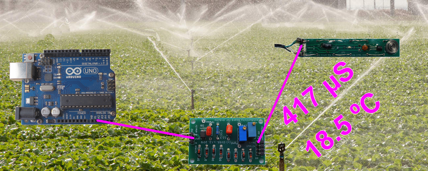
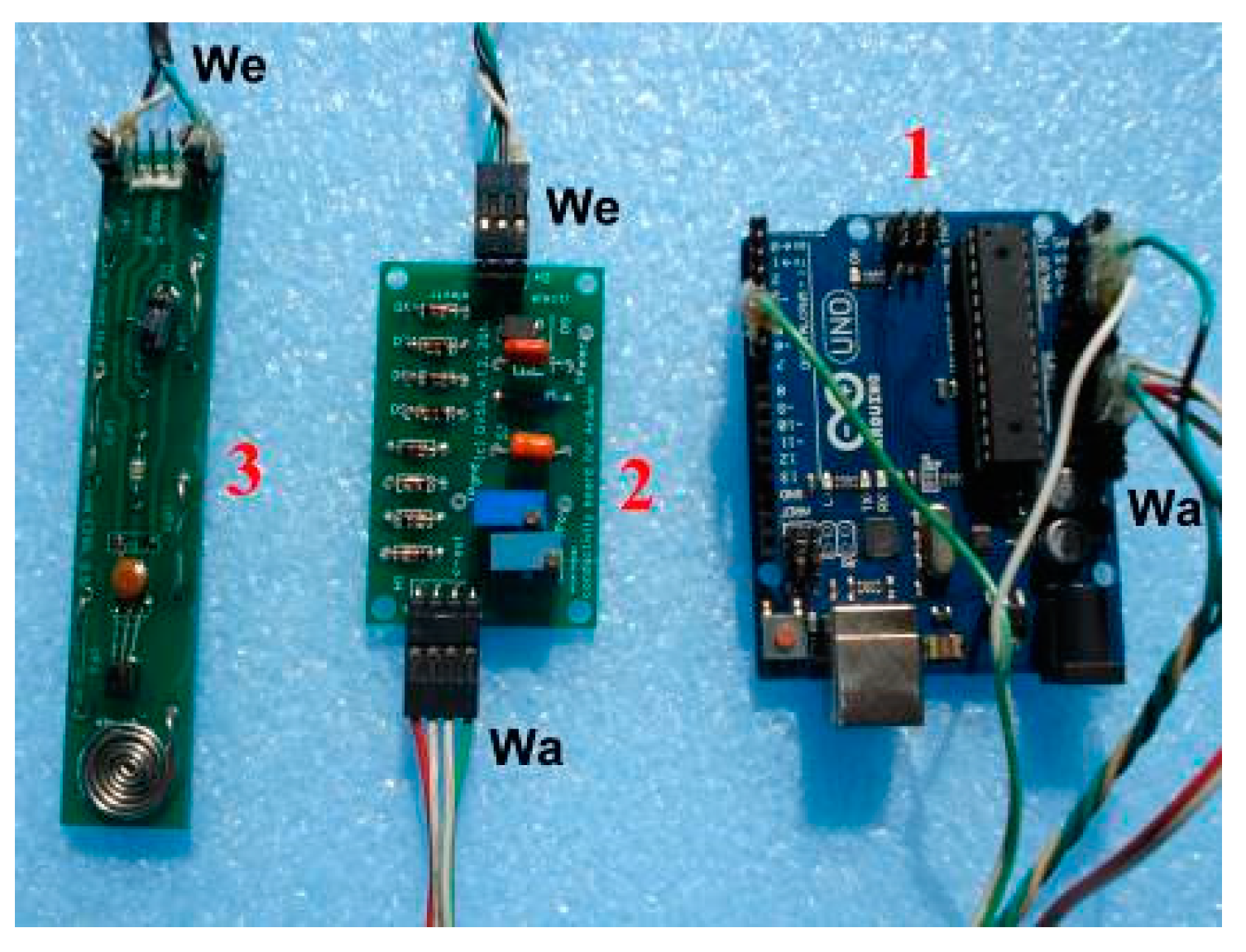
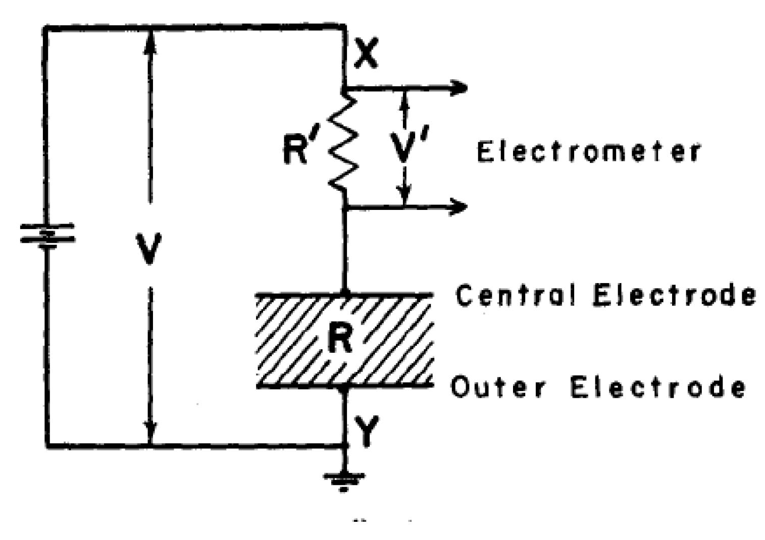
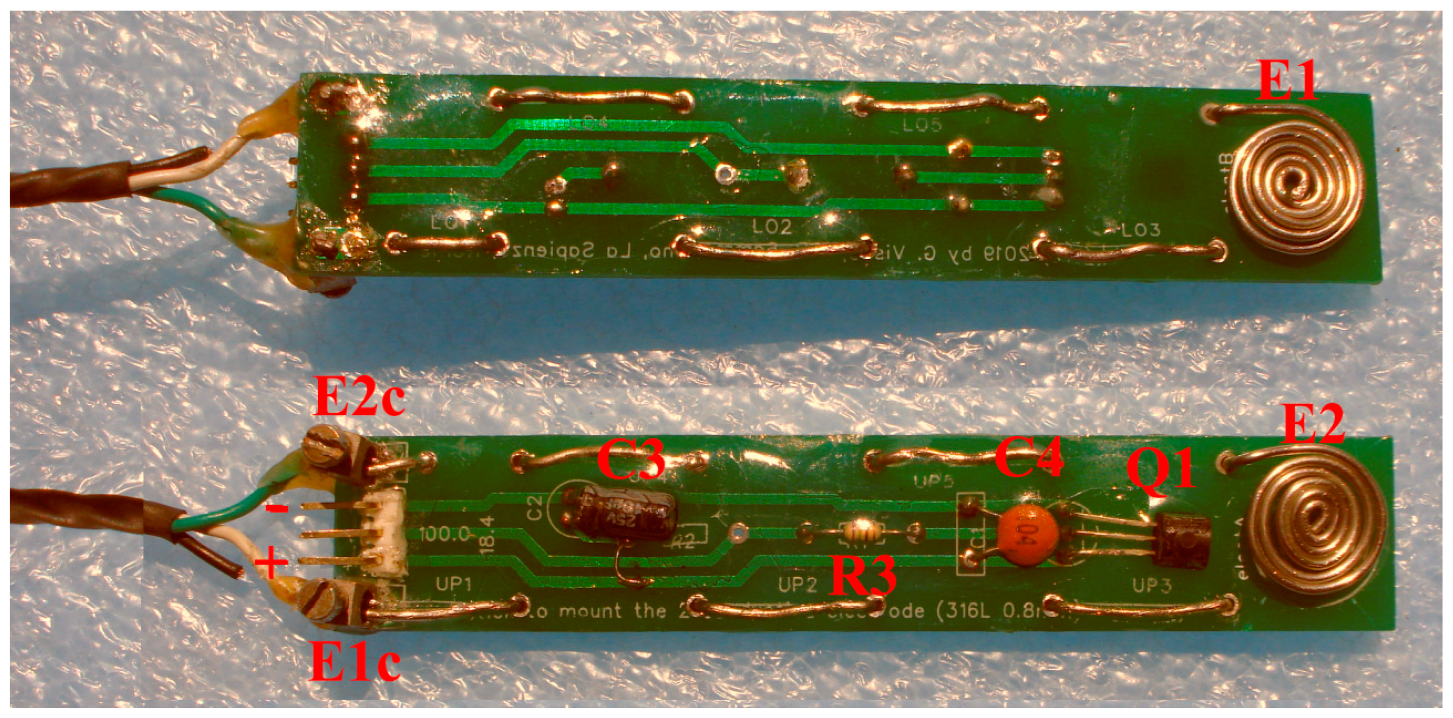
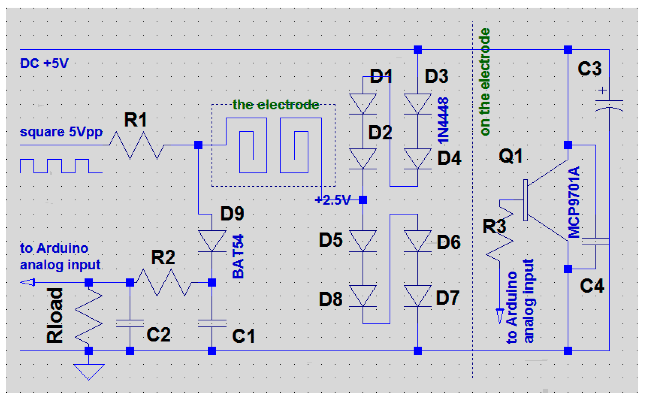
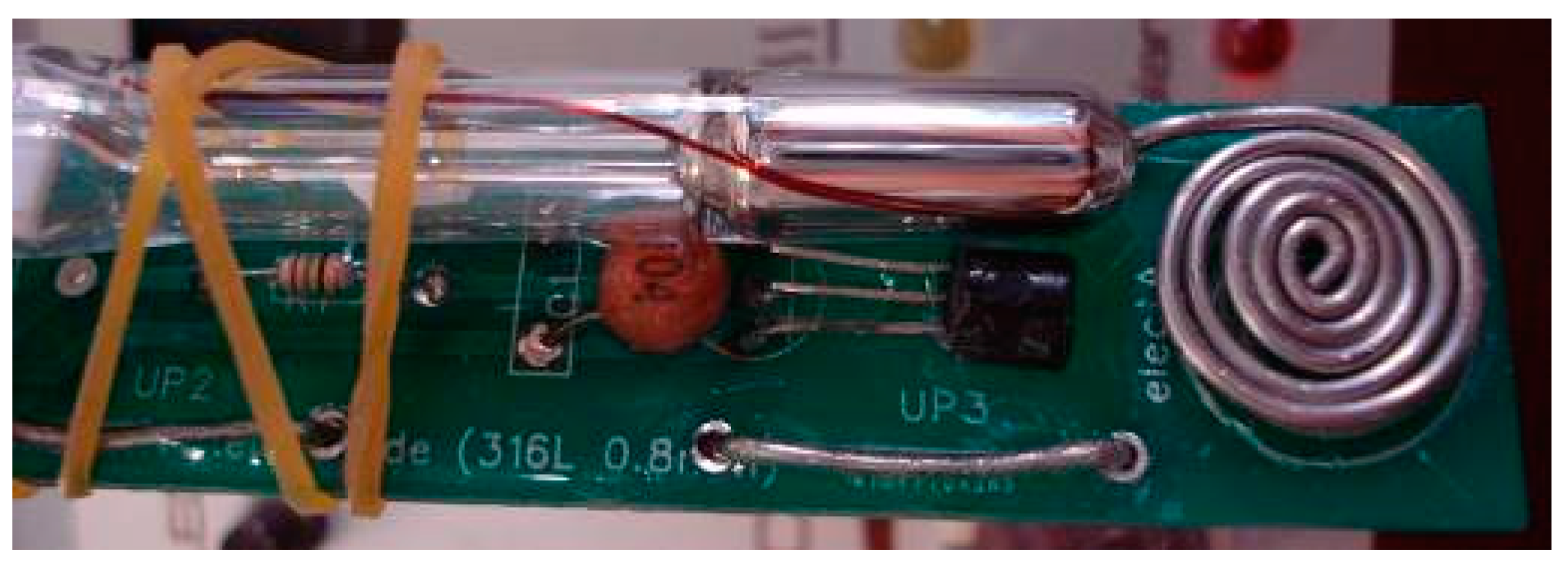
2.2. The Device Circuit

Arduino easily produces 5 V and 3.3 V Direct Current (DC, voltage) and pulses from 0 to 5 V at intervals of a few milliseconds up to some minutes; it also produces pulse signals with modulation (PWM), with frequencies of about 500 and 1000 Hz and a duty cycle of up to 256 levels, but the signal is a square wave between 0 and 5 V. Unfortunately, a symmetric voltage centered on zero (for example, −1.5, 0, +1.5 V) cannot be produced instead. As said above, the design of the electric circuit is based on the paper by Smith, as shown in Figure 2. It was modified by moving an electrode away to ground to obtain a current inversion in the solution, because a correct conductivity measurement requires a high frequency alternate voltage. In this project, of the 2 frequencies mentioned, the 1000 Hz frequency was used, which is easy to produce with some lines of code. In the shield we produced, placed between the Arduino and the electrodes, we see a row of 8 diodes in a series (see Figure 5). One side of the series is connected to the +5 V output from the Arduino, while the other side is connected to ground at 0 V. The current flowing in the diodes produces a voltage drop of 0.625 V on each of them, i.e., 2.5 V between the fourth and fifth diode. Precisely at this point, one of the electrodes is connected, from which a square wave between 0 and 5 V on one of the electrodes translates into a voltage of between −2.5 V and + 2.5 V towards the solution having shifted the potential of one of them.

The voltage varies depending on the resistance of the solution, and then, proportional to the current that passes between the electrodes, it is carried out by the Arduino and its microprocessor. The response curve of the conductivity values vs. the Arduino has a non-linear exponential trend similar to that of a radioactive decay. This is not a problem, because non-linear trends are common: as an example, see the NTCs used in 50% of the temperature measures [32]. In the Supplementary Materials, the equation of a typical NTC can be found in Figure S2 NTC-beta-equation.png, and the subtended response curve in Figure S3 ohm-temperature_100K-NTC.png, which are reported for comparison with the response of this instrument.

To obtain a continued inversion of polarity between the electrodes, an external shield/circuit is usually needed. Figure 5 shows the one we propose.

A detailed description of the circuit in Figure 5, describing the function of each individual component, can be found in the Supplementary Materials in the file Arduino-cond-temp-the-circuits.doc.

The software used to program the Arduino was IDE Release 1.8.9 (Arduino.cc, Monza, Italy). The sketch (file: Conduct-temp1.2.ino present in the Supplementary Materials) was written from scratch, without the use of a library or reusing another module. The sketch was split in part by relying on the use of routines and subroutines to obtain an easy-to-read listing and a more reliable object. The main routine is devoted to oversampling and decimation for the temperature and conductivity measurements.

We would like to present the instrument as an open-source project, so in the Supplementary Materials, a long text entitled “how to build it” is available, which describes step by step the acquiring of components, the soldering, the cable and wires to be used, and the installation of the software sketch, and contains some measures to check the obtained circuit (file: How-to-build-it-R2.doc in the Supplementary Materials). We used the Copyright under the terms of the GNU General Public License as published by the Free Software Foundation; version 4 of the following license: “Creative Commons Public License, CC-BY-NC-ND 4.0 EN”. Additionally, the schematics and drawings of the shield and electrode temperature module are under the same license.

3. Results and Discussions

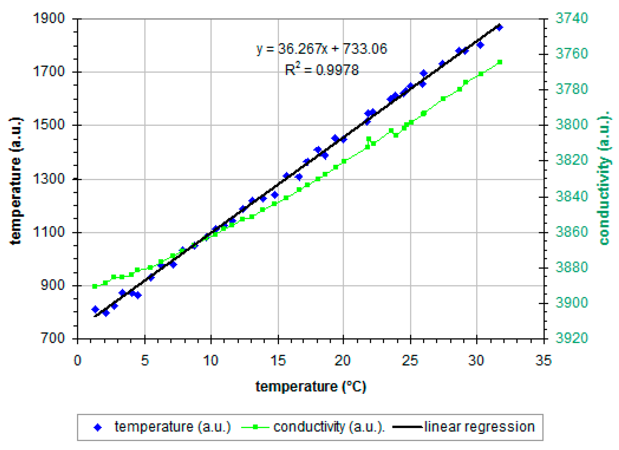
3.1. Temperature Sensor Calibration

The values in bits read from the Arduino for the temperature measurements, from the IC, must be transformed into values in °C through a comparative calibration: i.e., the IC sensor (mounted on the electrode) was placed very close to a common Hg thermometer (see Figure 6). Both were immersed in a thermostatic bath and the temperature varied manually from one grade up to thirty-five degrees at one-degree intervals.

Figure 7 shows the trend of the temperature calibration curve (Volt–Celsius) obtained from measurements in distilled water using the assembly shown in Figure 6. The relative equation, also reported in the figure, shows a linear trend, demonstrating the good quality of the measurements. Since it is well known that temperature has a strong effect on conductivity, we measured conductivity at the same time and illustrate, in the same figure, the trend of the signal, in a.u., as a function of temperature. Taking into account that we are using a non-traditional conductivity cell, it is not surprising that this trend is almost linear and decreasing; as a fact, the signal obtained from the Arduino decreases as conductivity increases and the trend is not linear but exponential (see Figure 8). In the Supplementary Materials, all the values obtained for the calibration are available (file: Temperature-Calib-1.2.xls).

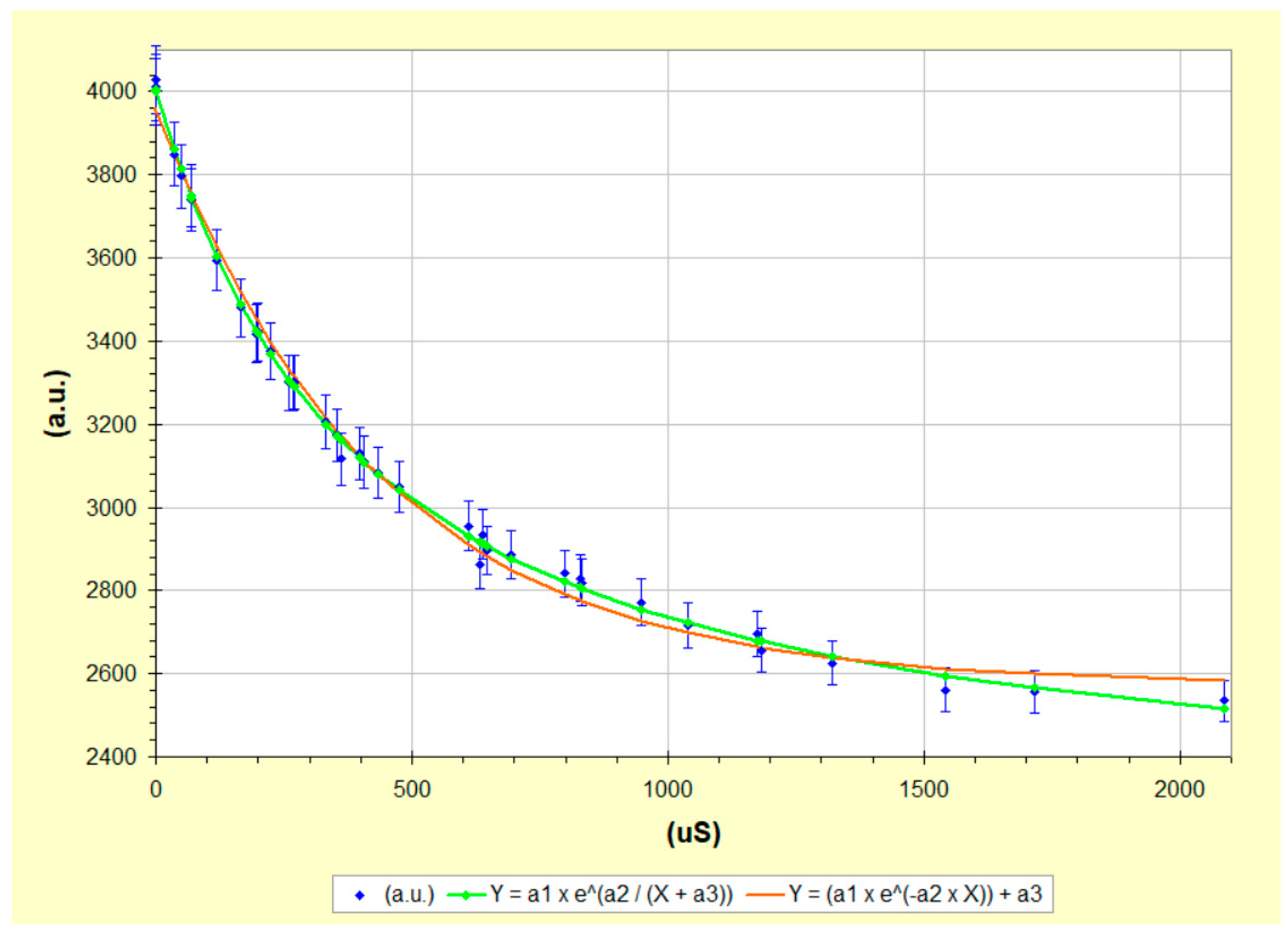
3.2. Conductivity Calibration

The calibration curve for conductivity was obtained using the method known as “secondary measurement standard”, which requires a large number of measures to obtain a reliable calibration curve [33]. With this aim in mind, we analyzed thirty-seven different solutions, with conductivities ranging from 2 to 2350 µS: three certified standards, tap water, deionized and distilled waters, and thirty-one commercial mineral waters. The zero-conductivity signal was obtained in air. Conductivity values declared on the labels of the mineral waters, measured at the source, were reported “at 20 °C”, i.e., after correction for the real temperature at the source, in order to ensure a correct comparison between them. In many cases, such values differed from those measured by us using both the proposed prototype and a commercial lab instrument. There are two main reasons for these differences. Even if, at the time of purchase, the mineral water’s expiry date was far off, the date of the official analysis was much earlier. The presence of carbon dioxide, as already said above, can distort the measurement; in practice, the smaller real surface of the electrode due to the presence of bubbles on their surface corresponds to a cell constant that is lower than that declared by the manufacturer and therefore automatically used by the conductivimeter. On such bases, we obtained our calibration curve looking for a correlation between values obtained by the Mettler lab instrument, used as a reference (Reference Conductimeter, CfR), and those obtained by our prototype under the same experimental conditions (20 °C and degassing pretreatment).

In the first four columns of

Table 1. List of the main data of the solutions used for the calibration.

Data Reported on the Label of the Mineral Waters and Standard				Experimental Values by
Sample	Spring Source (Location City)	Data of the Analysis	Conductivity Values (µS cm−1) (at °C T)	Lab Conductimeter (µS cm−1)	Arduino Prototype (a.u.)
In air	/	22 November 2020	0.001 (20)	0.0	4028.80
MilliQ	Millipore	22 November 2020	0.05 (20)	0.3	4010.20
Distilled	Still 3B	22 November 2020	2 (20)	1.2	3999.80
Sant’Anna 2016	Vinadio (CN)	23 March 2016	25.4 (20)	35.8	3849.00
S. Bernardo	Garessio CN)	21 May 2013	48 (20)	48.7	3796.80
Valmora	Rora (TO))	3 December 2013	60 (20)	67.8	3749.40
standard84	XS Instruments	May 2020	84 (25)	69.6	3739.40
Lievissima	Valdisotto (SO)	11 Sep 2017	118 (20)	117.6	3595.00
Fiuggi	Fiuggi (FR)	21 January 2012	187 (20)	165.1	3480.80
Rocchetta	Gualdo Tadino (PG)	11 July 2014	276.3 (20)	196.0	3418.00
Santa Croce	Castelpizzuto (IS)	24 October 2012	290 (20)	197.6	3422.00
Santa Croce	Castelpizzuto (IS)	1 September 2017	278 (20)	224.3	3376.40
Nestle Vera	San Giorgio in Bosco (PD)	29 May 2015	251 (20)	260.9	3299.60
Tullia	Sellano (PG)	3 November 2017	331 (20)	267.0	3299.00
Santa Vittoria	Montegrosso Pian Latte (IM)	23 October 2013	309 (20)	269.8	3300.80
Perla	Monte S. Savino (AR)	18 December 2013	1079 (20)	332.2	3204.80
Lete	Pratella (CE)	16 January 2017	1280 (20)	353.7	3173.80
Natia	Riardo (CE)	20 October 2016	390 (20)	362.1	3116.20
Sorgesana	Pratella, Ielo (CE)	9 January 2018	460 (20)	397.3	3129.60
Clivia	Gubbio (PG)	15 December 2016	451 (20)	407.2	3109.80
Tap water	Rome 00185	22 November 2020	563 (20)	432.7	3084.00
standard600	Sigma Aldrich		600 (25)	474.1	3049.40
Ferrarelle	Riardo (CE)	18 June 2014	1830 (20)	610.9	2955.40
Carrefour Ofelia	Contursi Terme (SA)	9 January 2013	619 (20)	633.6	2863.20
Nepi 2018	Nepi (VT)	30 August 2018	690 (20)	638.6	2934.80
Grazia	Acquasparta (TR)	12 July 2017	1624 (20)	647.3	2894.80
Santagata	Riardo (CE)	20 October 2016	1440 (20)	694.3	2885.00
Sangemini	San Gemini (TR)	26 October 2017	1365 (20)	799.9	2841.00
Claudia	Anguillara Sabazia (RM)	18 January 2017	940 (20)	828.9	2829.67
Vivia	Nepi (VT)	16 May 2014	767 (20)	832.3	2819.80
Uliveto 2019	Vicopisano (PI)	28 June 2019	1099 (20)	948.9	2771.80
Uliveto 2015	Vicopisano (PI)	19 June 2015	1104 (20)	1038.9	2717.20
Sveva	Rionero in Vulture (PZ)	14 April 2014	1780 (20)	1174.4	2695.80
standard1413	XS Instruments	February 2020	1413 (25)	1181.9	2656.00
Gaudianello	Rionero in Vulture (PZ)	5 October 2015	1504 (20)	1321.2	2625.40
4 + 1	Gaudianello + Essenziale	/	1392 (20)	1541.9	2561.40
1 + 1	Gaudianello + Essenziale	/	1598 (20)	1716.4	2555.20
Essenziale	Boario Terme (BS)	8 June 2016	2350 (20)	2086.8	2534.60

, the main data of the solutions used for the calibration are listed, while the last two columns show the data respectively obtained by the top-quality commercial laboratory apparatus for conductivity measurements and by our prototype when R1 = 1 KΩ and Rload = 10 MΩ (see Figure 5 for schematics).

The data from the two last columns of Table 1 were used to obtain the correlation chart shown in Figure 8; the two possible curves follow the experimental data, both of which demonstrate a non-linear trend.

Both of the curves in Figure 8 show an exponential trend. The orange (1) and green (2) curves better fit values at low conductivity and above 550 μS, respectively.

Y = a1 × e^(a2/(X + a3))

(1)

Y = (a1 × e^(−a2 × X)) + a3

(2)

It is always a good idea to obtain both equations to find the one that follows the data the best, due to the dependence on the shape of the electrodes and the values of the installed components. The coefficients a1, a2, a3, obtained in the described conditions, are reported in the Supplementary Materials (see the file Electrode-Calibration.xls). They can be used as a starting point to set the resolution using the “Solver” module of Microsoft Excel 2003 software, (Microsoft, Redmond, USA), as shown many times in the literature, as in [34].

Finally, to estimate the accuracy of the method for the calculation of conductivity proposed in this paper, a typical method of chemometrics was used: “Full Cross Validation” with the leave-many-out (leave-p-out) technique [35,36].

We have divided the samples in two groups, the training set and the test set, devoting to the latter about 15% of the values. We obtained an estimate of the accuracy of the method by means of residual values.

Thirty-one values were used for the training set and seven for the test set. The exponential equations were obtained from the training set and used to obtain the conductivity values for the test set. The percentage error was calculated using values measured by the lab instruments as real values. The results are reported in

Table 2. Accuracy, as percentage error, of the instrument, obtained using full cross validation and the leave-many-out technique.

Brand (Label)	Standard Value (µS cm−1)	Arduino Value (a.u)	Measured Value (µS cm−1)	Error (%)
Distilled	1.2	3999.8	1.6	33.3
Valmora	67.7	3749.4	67.6	−0.1
Santa Croce	197.6	3422.0	195.0	−1.3
Tullia	267.0	3299.0	262.8	−1.6
Sorgesana	397.3	3129.6	386.4	−2.8
Nepi	638.6	2934.8	601.8	−5.8
Sveva	1174.4	2698.8	1113.4	−5.2

.

The values in the table show that both the instrument and the analytical procedure adopted are suitable for the purpose for which the prototype was build up. With the exception of distilled water, the error was between 1 and 5%. The high error obtained for distilled water is not surprising taking into account that its conductivity is extremely low. The difficulty we experienced in measuring it, even with a quality laboratory instrument, and the differences in the resolution range led to high percentage error.

The accuracy and reproducibility values were calculated on the worst of three built instruments, the difference being due only to the precision of the electronic components used and the ‘similarity’ of the handmade, stainless-steel spirals. The differences were, however, less than 5% and, as usual, each new instrument must be calibrated.

4. Conclusions

The world’s water resources are diminishing and deteriorating in quality. Both water for human consumption and water for industrial use, especially in the agricultural sector, need to be monitored for quality; this concerns both water for direct use and industrial discharges. Salinity is one of the parameters that most influences water quality, and therefore, conductivity, as a related factor, is one of the main parameters needing to be controlled. Although the measurement of the electrical conductivity of an aqueous solution has been possible since the second half of the 19th century [37], and a wide range of conductivity meter models is currently available [38], it is difficult to find a conductivity meter that fully meets all the particular requirements of, for example, the agricultural sector [39]: ease of use, robustness, real-time data transmission, long-term stability, and, possibly, low cost [40]. At end of March 2023, 17,753 articles on Arduino were indexed on Scopus confirming its application in science as a multi-parameter sensor for marine research [41], but also in education [42]. The prototype for conductivity measures here presented fully meets our aims. It is surely economic (costing about EUR 15); simple to use both in lab and in situ; robust enough; has good, long-term stability; does not require frequent, particular care; and moreover, it allows for the continuous monitoring of the samples, causing little economic damage in the case of theft if placed in an external environment. Following the analytical procedure here described, good accuracy (error < 6%) and precision (RSD% about 5) were obtained, thanks to the temperature sensor equipped by the IC. On these bases, the prototype can be proposed as a valid alternative to more expensive instruments. In comparison with commercial portable instruments, we can assert that the price of the cheapest option is at least EUR 60, and their accuracy is ±2% of the full scale, meaning ±40 μS in the entire conductivity range and a 100% error for values ≤ 40 μS. The very low cost of the prototype is derived from the use of low-cost materials (steel electrodes, a small passive circuit/shield, free software), as well as to the handmade build. All of these characteristics, especially the last, allow us to suggest the buildup and use of the prototype for a laboratory didactic experience (one of our aims) that covers many topics such as basic electrochemistry, basic electronic components, software programming, and data treatment. To do this, students can follow the “how to build it” file, available in the Supplementary Materials, describing step by step the construction. All of the instruments are designed and distributed following the open-source dictates [43,44]. Even if a non-linear equation must be used to find conductivity from the values furnished by the Arduino (as for many other parameters), at present, many data processing software are available that allow for this problem to be easily solved; in the Supplementary Materials, we present one of them. Further, using the proposed calibration method, the measurement of the cell constant is not required because the software program does not need this information. Finally, the useful conductivity interval (ranging between about 1–3 and 2000 μs cm⁻¹ in the conditions here adopted) can be changed by changing the size of the spirals and the values of R1 and Rload.

References

1. Bakewell, F.C. On the conduction of electricity through water. J. Frankl. Inst. 1851, 52, 283. [Google Scholar] [CrossRef]
2. Rodger, J.W. The electric conductivity of pure water. Nature 1894, 51, 42–43. [Google Scholar] [CrossRef] [Green Version]
3. MacGregory, A.C. Determination of the electric conductivity of certain salt solutions. Phys. Rev. I 1895, 2, 361–372. [Google Scholar] [CrossRef] [Green Version]
4. Carneiro, L.R.S.; Garcia, D.C.S.; Costa, M.C.F.; Houmard, M.; Figueiredo, R.B. Evaluation of the pozzolanicity of nanostructured sol-gel silica and silica fume by electrical conductivity measurement. Constr. Build. Mater. 2018, 160, 252–257. [Google Scholar] [CrossRef]
5. Mendes, R.; Schimmer, O.; Vieira, H.; Pereira, J.; Teixeira, B. Control of abusive water addition to Octopus vulgaris with non-destructive methods. J. Sci. Food Agric. 2018, 98, 369–376. [Google Scholar] [CrossRef]
6. ISO 788:1985-2017; Water Quality—Determination of Electrical Conductivity. Into ISO/TC 147/SC2, Physical, Chemical and Biochemical Methods. International Organization for Standardization: Geneva, Switzerland, 1985.
7. Rabello, J.R.; Gonzáles, J.M.; Batista, J.R.; Silva, A.C.S.; Costa, E.J.X. A Simple, Effective, and Low-Cost System for Water Monitoring in Remote Areas Using Optical and Conductivity Data Signature. Water Air Soil Pollut. 2021, 232, 115. [Google Scholar] [CrossRef]
8. Gruda, N. Does soil-less culture systems have an influence on product quality of vegetables. J. Appl. Bot. Food Qual. 2009, 82, 141–147. [Google Scholar]
9. Lakhiar, I.A.; Jianmin, G.; Syed, T.N.; Chandio, F.A.; Buttar, N.A.; Qureshi, W.A. Monitoring and Control Systems in Agriculture Using Intelligent Sensor Techniques: A Review of the Aeroponic System. J. Sens. 2018, 2018, 8672769. [Google Scholar] [CrossRef] [Green Version]
10. Serrano-Finetti, E.; Aliau-Bonet, C.; López-Lapeña, O.; Pallàs-Areny, R. Cost-effective autonomous sensor for the long-term monitoring of water electrical conductivity of crop fields. Comput. Electron. Agric. 2019, 165, 104940. [Google Scholar] [CrossRef]
11. Blackmore, S. Precision Farming: An Introduction. Outlook Agric. 1994, 23, 275–280. [Google Scholar] [CrossRef]
12. El Nahry, A.H.; Ali, R.R.; El Baroudy, A.A. An approach for precision farming under pivot irrigation system using remote sensing and GIS techniques. Agric. Water Manag. 2011, 98, 517–531. [Google Scholar] [CrossRef]
13. Hamami, L.; Nassereddine, B. Application of wireless sensor networks in the field of irrigation: A review. Comput. Electron. Agric. 2020, 179, 105782. [Google Scholar] [CrossRef]
14. EN 16455:2014; Norm. Conservation of Cultural Heritage. Extraction and Determination of Soluble Salts in Natural Stone and Related Materials Used in and From Cultural Heritage. Slovenian Institute for Standardization: Newark, DE, USA, 2014.
15. Hooper, A.W. Computer control of the environment in greenhouses. Comput. Electron. Agric. 1988, 3, 11–27. [Google Scholar] [CrossRef]
16. García, L.; Parra, L.; Jimenez, J.M.; Lloret, J.; Lorenz, P. IoT-Based Smart Irrigation Systems: An Overview on the Recent Trends on Sensors and IoT Systems for Irrigation in Precision Agriculture. Sensors 2020, 20, 1042. [Google Scholar] [CrossRef] [Green Version]
17. Mattihalli, C.; Gedefaye, E.; Endalamaw, F.; Necho, A. Real Time Automation of Agriculture Land, by automatically Detecting Plant Leaf Diseases and Auto Medicine. In Proceedings of the 32nd International Conference on Advanced Information Networking and Applications Workshops (WAINA), Krakow, Poland, 16–18 May 2018. [Google Scholar] [CrossRef]
18. Hashim, N.M.Z.; Mazlan, S.R.; Abd Aziz, M.Z.A.; Salleh, A.; Ja’Afar, A.S.; Mohamad, N.R. Agriculture monitoring system: A study. J. Teknol. 2015, 77, 53–59. [Google Scholar] [CrossRef] [Green Version]
19. Urban, P.L. Open-Source Electronics As a Technological Aid in Chemical Education. J. Chem. Educ. 2014, 91, 751–752. [Google Scholar] [CrossRef]
20. Zachariadou, Z.; Yiasemides, K.; Trougkakos, N. A low-cost computer-controlled Arduino-based educational laboratory system for teaching the fundamentals of photovoltaic cells. Eur. J. Phys. 2012, 33, 1599–1610. [Google Scholar] [CrossRef]
21. Grinias, J.P.; Whitfield, J.T.; Guetschow, E.D.; Kennedy, R.T. An Inexpensive, Open-Source USB Arduino Data Acquisition Device for Chemical Instrumentation. J. Chem. Educ. 2016, 93, 1316–1319. [Google Scholar] [CrossRef] [Green Version]
22. Salvador, C.; Mesa, M.S.; Durán, E.; Alvarez, J.L.; Carbajo, J.; Mozo, J.D. Open ISEmeter: An open hardware high-impedance interface for potentiometric detection. Rev. Sci. Instrum. 2016, 87, 055111. [Google Scholar] [CrossRef]
23. Cao, T.; Thompson, J.E. Portable, Ambient PM2.5 Sensor for Human and/or Animal Exposure Studies. Anal. Lett. 2017, 50, 712–723. [Google Scholar] [CrossRef]
24. González, P.; Pérez, N.; Knochena, M. Low cost analyzer for the determination of phosphorus based on open-source hardware and pulsed flows. Química Nova 2016, 39, 305–309. [Google Scholar] [CrossRef]
25. Wishkerman, A.; Wishkerman, E. Application note: A novel low-cost open-source LED system for microalgae cultivation. Comput. Electron. Agric. 2017, 132, 56–62. [Google Scholar] [CrossRef]
26. Alimorong, F.M.L.S.; Apacionado, H.A.D.; Flores Villaverde, J. Arduino-based Multiple Aquatic Parameter Sensor Device for Evaluating pH, Turbidity, Conductivity and Temperature. In Proceedings of the 12th IEEE International Conference on Humanoid, Nanotechnology, Information Technology, Communication and Control, Environment, and Management, HNICEM 2020, Manila, Philippines, 3–7 December 2020. [Google Scholar]
27. Nayyar, A.; Puri, V. A review of Arduino board’s, Lilypad’s & Arduino shields. In Proceedings of the 2016 3rd International Conference on Computing for Sustainable Global Development (INDIACom), New Delhi, India, 16–18 March 2016; pp. 1485–1492, ISSN 09737529. [Google Scholar]
28. Carminati, M.; Stefanelli, V.; Luzzatto-Fegiz, P. Micro-USB Connector Pins as Low-Cost, Robust Electrodes for Microscale Water Conductivity Sensing in Oceanographic Research. Procedia Eng. 2016, 168, 407–410. [Google Scholar] [CrossRef] [Green Version]
29. Smith, L.G. On the Calibration of Conductivity Meters. Rev. Sci. Instrum. 1953, 24, 998. [Google Scholar] [CrossRef]
30. Aswin Kumer, S.V.; Kanakaraja, P.; Mounika, V.; Abhishek, D.; Praneeth Reddy, B. Environment water quality monitoring system, Materials Today. In Proceedings of the International Conference on Materials, Manufacturing and Mechanical Engineering for Sustainable Developments, ICMSD 2020, Chennai, India, 19–20 December 2020; Volume 46, pp. 4137–4141. [Google Scholar]
31. D’Ausilio, A. Arduino, A low-cost multipurpose lab equipment. Behav. Res. 2012, 44, 305–313. [Google Scholar] [CrossRef] [PubMed] [Green Version]
32. EPCOS AG, TDK. NTC Thermistor, General Technical Information; TDK: Tokyo, Japan, 2018. [Google Scholar]
33. JCGM 200:2012; Vocabulaire International de Métrologie—Concepts Fondamentaux et Généraux et Termes Associés (VIM) (p. 48, 5.5 note 2). BIPM: Paris, France, 2008.
34. Pinder, J.P. An Excel Solver Exercise to Introduce Nonlinear Regression. Decis. Sci. J. Innov. Educ. 2013, 11, 263–278. [Google Scholar] [CrossRef]
35. Lorber, A.; Kowalski, B.R. Alternatives to cross-validatory estimation of the number of factors in multivariate calibration. Appl. Spectrosc. 1990, 44, 1464–1470. [Google Scholar] [CrossRef]
36. Besalú, E. Fast computation of cross-validated properties in full linear leave-many-out procedures. J. Math. Chem. 2001, 29, 191–204. [Google Scholar] [CrossRef]
37. Lubert, K.H.; Kalcher, K. History of Electroanalytical Methods. Electroanalysis 2010, 22, 1937–1946. [Google Scholar] [CrossRef]
38. Gray, J.R. Conductivity Analyzers and Their Application. In Environmental Instrumentation and Analysis Handbook; Down, R.D., Lehr, J.H., Eds.; John and Wiley and Sons: Hoboken, NJ, USA, 2004; p. 491. [Google Scholar]
39. Velazquez, L.A.; Hernandez, M.A.; Leon, M.; Dominguez, R.B.; Gutiérrez, J.M. First advances on the development of a hydroponic system for cherry tomato culture. In Proceedings of the 10th International Conference on Electrical Engineering, Computing Science and Automatic Control (CCE), Mexico City, Mexico, 30 September–4 October 2013. [Google Scholar]
40. Matese, A.; Di Gennaro, S.F.; Zaldei, A. Agrometeorological monitoring: Low-cost and open-source—Is it possible? Ital. J. Agrometeorol. 2015, 20, 81–88. [Google Scholar]
41. Poquita-Du, R.C.; Morgia Du, I.P.; Todd, P.A. EmerSense: A low-cost multiparameter logger to monitor occurrence and duration of emersion events within intertidal zones. HardwareX 2023, 14, 00410. [Google Scholar] [CrossRef] [PubMed]
42. Goncalves, A.M.B.; Freitas, W.P.S.; Calheiro, L.B. Resources on physics education using Arduino. Phys. Educ. 2023, 58, 033002. [Google Scholar] [CrossRef]
43. Perens, B. Open Source Hardware (OSHW) Definition 1.0, Open Source Hardware Association. 2010. Available online: https://www.oshwa.org/definition/ (accessed on 10 February 2023).
44. Perens, B. Open Source Hardware (OSHW). 2010. Available online: https://freedomdefined.org/OSHW (accessed on 10 February 2023).
Figure 1. Complete conductivity instrument. 1: Arduino board, 2: self-made shield, 3: conductivity cell equipped with a temperature sensor, We: wires connecting the shield to the conductivity cell, Wa: wires connecting the shield to Arduino.
Analytica 04 00017 g001
Figure 2. Our starting point in building an Arduino-based conductivity meter (L.G. Smith paper, page 998 [29]).
Analytica 04 00017 g002
Figure 3. The 2 sides of the PCB electrodes. E1 and E2: inox spiral, Q1: temperature sensor, C3 and C4: stabilizing capacitors, R3: resistor for impedance matching, E1c and E2c: cables for electrodes, −/+: power supply and output signal for Q1.
Analytica 04 00017 g003
Figure 4. Waveform detected by the oscilloscope attached to the electrodes (pins E1c and E2c) for the 84 µS standard. We note the square wave and applied frequency of 980 Hz instead of the theoretical 1000 Hz, and the peak voltage of 2.24 V, i.e., 0.79 V RMS. Frequency and voltage can also be derived from the axis scale as 200 µS and 500 mV.
Analytica 04 00017 g004
Figure 5. The complete schematics of the proposed instrument, with the shield board on the left and the electrode board on the right. Each component is described in the text.
Analytica 04 00017 g005
Figure 6. Assembly of the Hg thermometer on the IC, adopted for the temperature calibration.
Analytica 04 00017 g006
Figure 7. Calibration curve and relative equation of the straight line obtained for temperature using the assembly shown in Figure 6 for measurements in distilled water (blue dots). The simultaneous trend of the conductivity signal as a function of temperature is also shown by the green dots.
Analytica 04 00017 g007
Figure 8. Calibration curve obtained using all the 38 samples: in blue, the experimental points; in green and in orange, two possible curves fitting the data. The relative equations are reported in the legend.
Analytica 04 00017 g008