Article

A Computational Fluid Dynamics Analysis of Hydrogen Leakage and Nitrogen Purging of a Solid Oxide Fuel Cell Stack

by
Rasmus Dockweiler Sørensen
and
Torsten Berning
*
Department of Energy Technology, Aalborg University, 9220 Aalborg, Denmark
*
Author to whom correspondence should be addressed.
Hydrogen 2023, 4(4), 917-931; https://doi.org/10.3390/hydrogen4040054
Submission received: 7 September 2023 / Revised: 20 October 2023 / Accepted: 24 October 2023 / Published: 4 November 2023
(This article belongs to the Special Issue Feature Papers in Hydrogen (Volume 2))

Abstract

:
A computational study of the nitrogen purging of a solid oxide fuel cell stack enclosed in a hot box is presented. The stack operates on ammonia as a fuel, and in the case of a hydrogen leakage, the entire compartment is immediately purged with nitrogen to ensure that there are no regions with high oxygen concentrations. In addition to this, the speed at which a hydrogen leak can be detected is determined. The results are then compared to a case with a relocated nitrogen inlet. A computational fluid dynamics (CFD) model is developed using the Reynolds-averaged Navier–Stokes equations for compressible flow in combination with conservation of energy and species equations in OpenFOAM. The results suggest that for the maximum concentration of oxygen to be below 5%, the hot box should be purged for 35 s, corresponding to 1.1 kg of nitrogen, if the hot box was already heated. If the hot box was at T = 300 K, it should be purged for 95 s, corresponding to 3.0 kg of nitrogen. The purge of the heated hot box results in a heat loss of 18 kW on average. A leak could be detected in 3.2 s during open circuit voltage tests. Changing the location of the outlet does not affect the cold purge, but results in a minimum purge period of 48 s during the hot purge, and the leak could be detected in 2 s. This paper demonstrates how CFD methods can be employed in order to address questions related to hydrogen safety.

1. Introduction

Fuel cell (FC) technology will become a key technology in order to reach the climate goals set by the European Union [1], the Paris Agreement [2] and the International Maritime Organization IMO [3]. Emissions from fuel cells are considered net zero, provided that the fuels are produced using sustainable technologies. Emissions of products, such as NOx and SOx, are considered negligible when using fuel cells [4]. Fuel cells commonly use hydrogen as their fuel, but other fuels, carrying hydrogen, such as methanol and liquid ammonia are also being investigated. One of the reasons is the low volumetric energy density of hydrogen compared to traditional fuels. For hydrogen to be utilized as a fuel, it has to be stored at a high pressure (≈700 bar) or in the liquid phase (≈−250 °C), and it will still have a low volumetric energy density compared to other fuels [5]. In addition to this, there is still a lack of a distribution infrastructure of hydrogen, compared to e.g. methanol [6] or ammonia that can be used as direct fuel in high temperature fuel cells [7]. Ammonia has the advantage of having an existing infrastructure, large production and proven safety procedures. Another benefit of ammonia, compared to hydrocarbons used in FCs, is that the only emission is water. Finally, ammonia can be created via various sustainable ways, as summarized in Figure 1. According to a recently published report by the European Marine Safety Agency, there could be enough green ammonia based on hydrogen generated via electrolysis to power the maritime fleet alone by 2040, although this sector will compete with others for green hydrogen [8]. According to the same report, engine developments related to the use of ammonia are ongoing. However, issues related to concerns on nitrogen oxide (NO x ) and nitrous oxide (N 2 O) emissions, as well as the detrimental effects of ammonia slip from engines would need to be addressed [8].
A different way of harvesting the energy of ammonia is to employ solid oxide fuel cells (SOFCs) to generate electricity. For the operation of SOFCs using ammonia, ammonia is almost completely cracked at 400 °C [7], meaning the high operational temperature of SOFCs in the range of 600–800 °C is very suitable. The practical efficiency when using ammonia was found to be around 40% in the first 1500 h of operation at a current density of 1 A/cm 2 [7]. As the test conditions were not optimised, even higher efficiencies should be achievable.
In previous work studying SOFCs operating on ammonia, preliminary studies assessed the feasibility of the concept and demonstrated that no production of thermal NOx occurs in the anode [9,10,11]. The degradation rates of SOFCs operating on both hydrogen and ammonia were investigated by Cinti et al., and they found similar values of 11.7 and 12.5 mV/100 h, respectively, at a temperature of around 745 °C [12].
The high operating temperature raises a question of safety, as hydrogen that invariably results from ammonia cracking has an autoignition temperature of 510 °C [13]. The lower flammable level (LFL) of hydrogen is the lowest in the upward direction at 4% in air at standard temperature and pressure [13]. The lower explosive level (LEL) is a hydrogen concentration of 10%. The lower oxygen concentration (LOC) is 5% at standard temperature and pressure. The lower limits decrease at higher temperatures [14].
In recent years, the Danish company Alfa Laval in Aalborg has investigated ammonia-fueled SOFCs for maritime applications. For the SOFC system, an insulated hot box is used that contains an air-air heat exchanger, a fuel-fuel heat exchanger, an electric heater and the SOFC stack. Figure 2 is a CAD model of the hot box. It can be seen that the nitrogen inlet is at the front, lower right and the outlet at the upper back. To avoid explosive scenarios the hot box is purged with nitrogen. In case of a leak, a sensor is equipped at the outlet, detecting hydrogen concentrations above 0.4%.
Several authors have investigated the risk of different hydrogen leaks using computational fluid dynamics (CFD), including hydrogen leaks from hydrogen fuelling stations [15], a detonation after a hydrogen leak in an enclosure [16] and hydrogen leaks in a laboratory [9], vehicles [10] and a ventilation facility [11].
In reference [15], Kikukawa et al. simulated a hydrogen leak from a fueling station nozzle. FLUENT 6.2 software (ANSYS Inc., Canonsburg, PA, USA) was used to set up the CFD model. The Reynolds-averaged Navier–Stokes (RANS) equations, using the standard k- ε as a turbulence model, for a compressible flow were solved, in combination with the conservation of species for an ideal gas mixture. The effects of a barrier were investigated, and it was concluded that a barrier would enhance the diffusion and shorten the travel distance of the hydrogen.
In reference [9], a hydrogen leak from a pipe in a laboratory was simulated. Ansys CFX was used to set up the CFD model. The RANS method was used, applying the Shear Stress Transport (SST) k- ω model due to supersonic flow. The transient terms were discretised using the second-order backward Euler scheme. All of the species, i.e., hydrogen, oxygen and nitrogen, were modelled individually. The ideal gas equation was used as the equation of state. Heat transfer at the walls was also included in this simulation. Prior to the hydrogen leakage simulation, the flow field in the laboratory in a normal state was simulated. These results were then used as the initial state of the leak simulation. The leak was simulated as a time-dependent flow. Experimental tests showed that a hydrogen leak would be detected 2–3 s after its occurrence by a sensor detecting a hydrogen concentration above 0.4%.
In reference [11], CFD in combination with experimental data was used to analyse a hydrogen leak in a semi-closed ventilation facility. The CFD code STARCCM+ was used. The turbulence was modelled using the realisable k- ε model in combination with the conservation of species and energy. The simulation was run at different ventilation flow rates and hydrogen leak pressures.
It is noted that all of the above studies relied on commercial tools that require the purchase of a user license. In contrast, OpenFOAM is a free, open-source CFD software (OpenFOAM v10) developed primarily by OpenCFD Ltd in 2004. It thus has the advantages of having no license cost, an ever-growing user base and complete access to the source code. The possibility of using OpenFOAM for gas dispersion was investigated by Mack and Spruijt [17] and Fiates and Vianna [18].
The former authors validated OpenFOAM-2.1-0 for heavy gas dispersions and compared their results to ANSYS Fluent [17]. The model solved the RANS equations in combination with the conservation of species and energy, without considering reactions. The turbulence model used was the standard k- ε model. It was concluded that OpenFOAM was suitable to predict heavy gas dispersions at least on par with commercial codes.
Fiates and Vianna [18] used OpenFOAM for gas jet and gas dispersion modelling. The model solved the RANS equations in combination with the conservation of species and energy, without considering reactions. The convection terms were discretised using central difference and temporal upwind diffusion using the first-order Euler scheme. Pressure–velocity coupling was performed via the PIMPLE algorithm. Similar to this work, the standard k- ε and SST k- ω were investigated as turbulence models. No significant difference was found between the two models, and, importantly, good agreement with experimental data was obtained.
In the present article, OpenFOAM has been employed in order to:
  • Simulate the purging of the hot box with nitrogen and assess the amount of nitrogen required and how long it takes until the maximum oxygen concentration reaches 5%, given that it is filled with air at atmospheric pressure and initial temperatures of 800 °C and 300 °C, respectively.
  • Assess the cooling effect of the purge on the hot box.
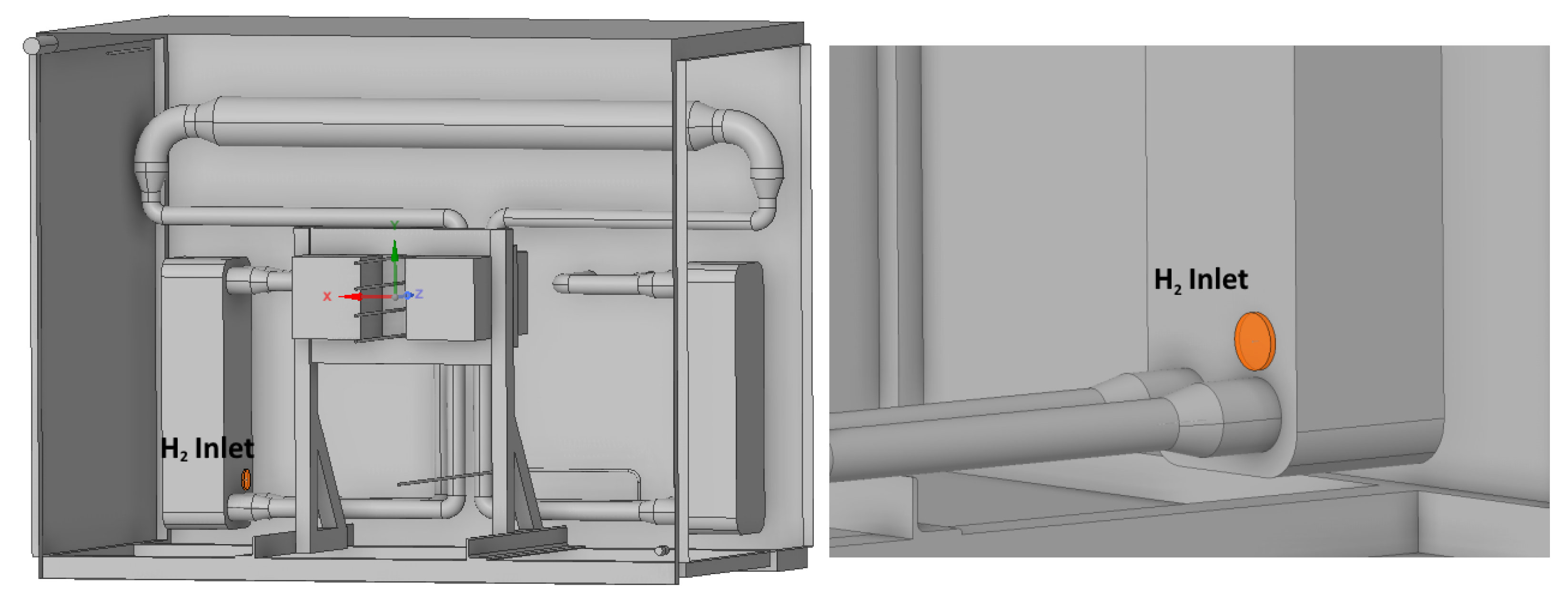
  • Assess how long it takes for the hydrogen concentration to exceed 0.4% at the outlet if a leak occurs from the fuel-to-fuel heat exchanger during the OCV test.
  • Compare the above results with a case where the outlet of the hot box has been relocated. The defined leak location is illustrated in Figure 3 and the relocated outlet is illustrated in Figure 4.

2. Mathematical Model

2.1. Main Assumptions

The list below gives an overview of the main assumptions:
  • The gases are assumed as ideal.
  • The flow is assumed as incompressible.
  • Buoyancy effects are neglected during the purge simulations.
  • For the modelling of diffusive transport, both the laminar and turbulent Schmidt numbers are equal to one.

2.2. Governing Equations

The solvers used in this project are ReactingFoam and RhoReactingBuoyantFoam, which are transient solvers that can handle turbulent, compressible and reacting flows. The governing equations solved are the conservation equations for mass, momentum, species and energy. The conservation equations can be written as stated in Equations (1)–(5) [19,20].
Continuity
ρ t + · ( ρ u ) = 0
Momentum
( ρ u ) t + · ( ρ u u ) = p + ρ g + τ
τ = 2 3 μ ( · u I + μ [ u + ( u ) T ]
Species
( ρ y i ) t + · ( ρ y i u ) = · ( μ eff y i )
Energy
( ρ h ) t + · ( ρ u h ) + ( ρ K ) t + · ( ρ u K ) = p t + · ( α eff h ) + ρ u · g
where ρ is the density, t is the time, u is the velocity vector, p is the pressure, g is the gravitational acceleration vector, τ is the stress tensor, μ is the dynamic mixture viscosity, I is the identity matrix, y i is the mass fraction of species i, h is the enthalpy, K is the kinematic energy and α eff is the effective thermal diffusivity.
The conservation of species uses the effective viscosity, instead of the effective mass diffusivity, given as ν eff = ν lam + ν turb . This results in the assumption that the laminar and turbulent Schmidt numbers, S c lam and S c turb , are equal to one, as stated above. The effect of the turbulent Schmidt number has been reviewed by Gualtieri et al. [21]. No universal method to determine the value was concluded, but fitted values for different flow configurations were found and suggest that the value varies locally.
In this work, the conservation of species (Equation (4)) is modified to use a specified constant value of S c turb and S c lam , meaning D eff is given as:
D eff = ν lam S c lam + ν turb S c turb
where D eff is the effective mass diffusivity.
During the purge, buoyancy is neglected ( g = 0 ). In OpenFOAM, the pressure gradient and gravity force terms are rearranged as [22]:
p + ρ g = p rgh ( g · r ) ρ
Here, p rgh = p ρ g · r and r is the position vector.

2.3. Turbulence Models

The diameter of the nitrogen purge inlet is 18.5 mm. Subtracting the volume of the components of the HB, the volume of the HB is 1.69 m 3 . The volume flow of nitrogen corresponds to the total volume over a minute. This results in the inlet Reynolds number ( R e ) given in Equation (8):
R e = 4 V ˙ π D ν = 129 , 000
where V ˙ is the volume flow, D is the diameter and ν is the kinematic viscosity of nitrogen. The Reynolds number is above 10,000; this means that the entering flow is fully turbulent. The characteristic length of the hot box is however much larger than that of the inlet, meaning the turbulence is expected to have little impact.
During a leak, R e leak , in < 2300 , meaning the flow is laminar. A laminar simulation is therefore also compared in this case.
In the literature, the commonly used turbulence models are the SST k ω , the standard k ε and the realisable k ε models [9,10,11,15,17,18]. Based on the literature, this suggests that a RANS model is sufficient and LES is not required.
In this paper three different turbulence models are tested, including the standard k ε , the SST k ω and the k ε ϕ f model. The transport equations for the standard k ε model are
( ρ k ) t + ( ρ k u ) = · ( ρ D k k ) + P ρ ε
( ρ ε ) t + ( ρ ε u ) = · ( ρ D ε ε ) + C 1 ε k ( P + C 3 2 3 k · u ) C 2 ρ ε 2 k
where D k is the effective diffusivity of k, P is the turbulent kinetic energy production rate, D ε is the effective diffusivity of ε and C 1 2 are model coefficients. The standard coefficients of OpenFOAM are used. The SST k ω model substitutes ω = ε / k into Equation (10) and introduces the blending function F 1 . The transport equation is given as [22]:
( ρ ω ) t + ( u ρ ω ) = · ( ρ D ω ω ) + ρ γ G ν 2 3 ρ γ ω ( u ) ρ β ω 2 ρ ( F 1 1 ) C D k ω New term + S ω
where D ω k ω is the effective diffusivity, γ and β are model coefficients, G is the turbulence generation and S ω is a source term.
The difference between the transport equation of ε and ω is the term ρ C D k ω . When F 1 = 1 it results in the k ω model and if F 1 = 0 it is the k ε model.
The k ε ϕ f model introduces the transport equation for ϕ , which is the normalized wall-normal fluctuating velocity scale, and f, the elliptic relaxation factor. The transport equations are, respectively [22,23]:
ρ ϕ t + · ( ρ u ϕ ) 2 ( ρ D ϕ ϕ ) = ρ f ρ G k 2 3 · u 2 ν ( ϕ · k ) k σ k ϕ ϕ
2 f = 1 L 2 f ( C f 1 1 ) ϕ 2 3 T C f 2 G k + C f 2 2 3 · u 2 ν · ϕ k k ν 2 ϕ 1 L 2
where T and L are the time and length scale used by the k ε ϕ f model.

2.4. Boundary and Initial Conditions

Three scenarios are to be investigated: nitrogen purge of the hot box filled with hot air, nitrogen purge of the hot box filled with ambient air and a fuel leak during OCV testing. The most important boundary and initial conditions will be determined.
For the inlet, a fixed volume flow of 1669 L/min during the purge simulations is applied. This volume flow corresponds to the entire volume of the hot box over 60 s.
During the leak simulation, a fixed mass flow of 1.35 kg/s is used.
Fixed temperatures of 300 K and 1073 K are used for the components and at the inlet during the purge simulations and leak simulations, respectively. At the walls and outlet, a zero gradient is used, corresponding to adiabatic conditions ( ϕ / n = 0 ).
The molar composition at the inlet is pure nitrogen during the purge. During the purge, it is composed of x H 2 = 0.6 and x N 2 = 0.4 . Initially, inside the hot box, the composition is x N 2 = 0.79 and x O 2 = 0.21 during the purge and x N 2 = 0.97 and x O 2 = 0.03 during the leak.
Finally, the inlet values of the turbulence parameters are the standard boundary conditions used in the OpenFOAM tutorials. Turbulent intensities of 0.034 and 0.01 are defined at the inlet during the purge and leak, respectively. Similarly, a mixing length of l m = 0.07 D is defined at the inlet during the purge and leak, respectively [24].
At the outlet, the pressure is fixed at 0.995 bar, and elsewhere a zero gradient is used. During the leak simulation, buoyancy is considered, introducing p rgh . In this case, p rgh uses the boundary conditions of p and p is calculated at the boundaries based on p rgh .

2.5. Numerical Verification

The PIMPLE algorithm was used, which is a combination of the SIMPLE and PISO algorithm [24]. The maximum Courant number ( C o = Δ t 2 V i j f a c e s u i · n i , j A i , j ) used during the purge simulations is C o max = 50 and C o max = 0.5 during the leak simulations. The mean C o is however much lower (in the order of 1 × 10 2 during the purge). Different values of C o max were tested to ensure the results were independent of the time step. The time derivatives are discretised using first-order Euler scheme. The upwind scheme is used for the discretisation of the turbulent advection terms. The rest of the terms are discretised using second-order accurate schemes. Different schemes were tested for the simulations.
Grid-independent studies were carried out for the purge in the case of a high initial temperature and for the leak. The inspected parameters for the purge were the volume averaged x O 2 in the entire hot box, near the fuel cell stack and near the fuel–fuel heat exchanger, | u | out and p in . The inspected parameters for the leak were the volume-averaged x H 2 concentration in the entire hot box, the mean x H 2 at the outlet and | u | out . The resulting mesh had a size of 7.3 × 10 5 and 6.5 × 10 5 cells for the purge and leak simulations, respectively.

3. Results and Discussion
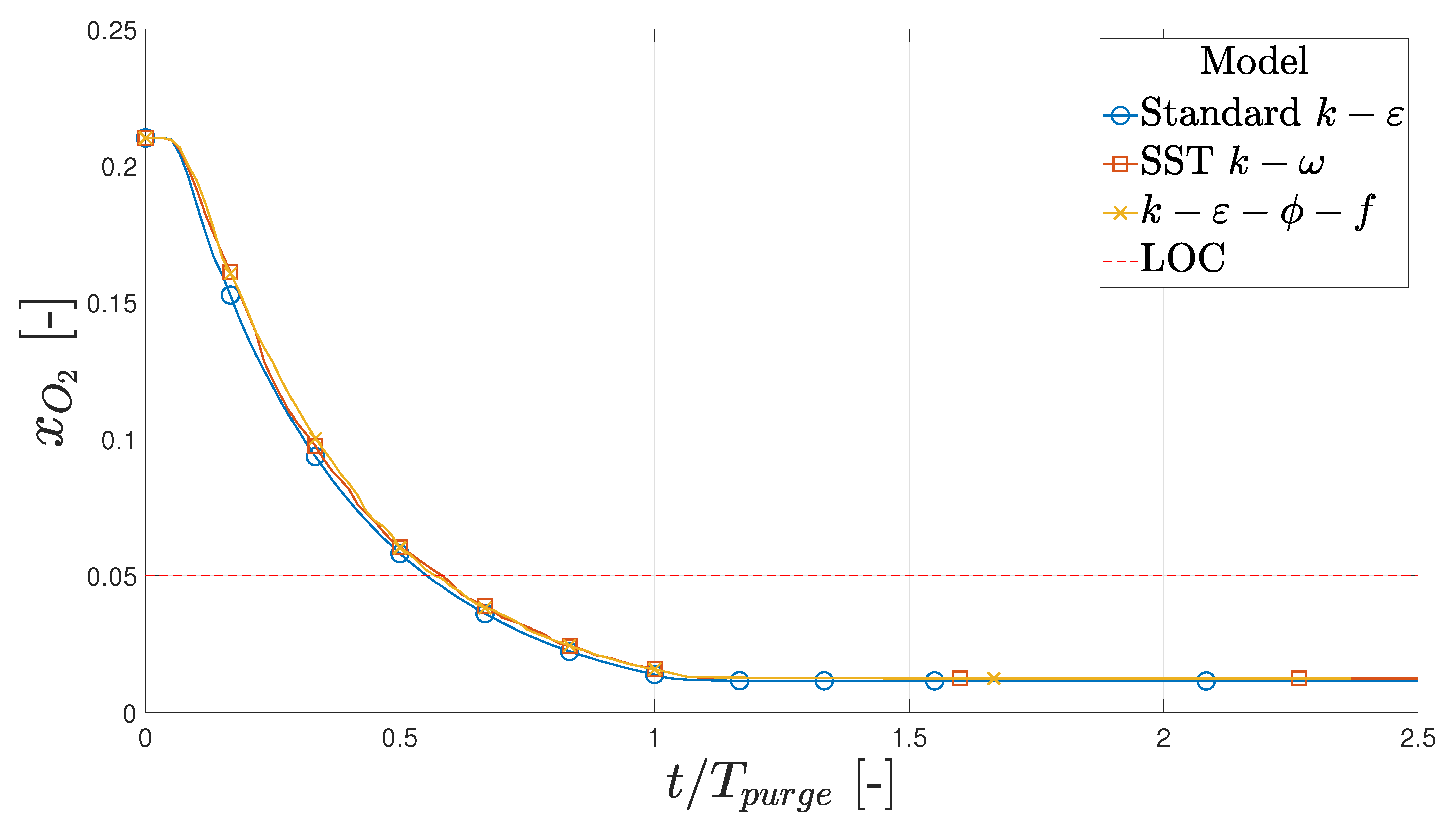
3.1. Hot Purge

The simulations for this purge use S c lam = S c turb = 1 . The maximum molar oxygen concentration is illustrated in Figure 5 for all three turbulence models. The time during the purge simulations was non-dimensionalised by dividing by T purge = 60 . This is the initial purge period suggested by Alfa Laval and the period for a volume of nitrogen to be injected corresponding to the volume of the hot box.
The maximum x O 2 is below the LOC when the purge is already 60% complete. This corresponds to 1.33 kg of nitrogen being used. The threshold is crossed first for the standard k ε model and lastly for the SST k ω model in the period 0.552 < t / T purge < 0.582 .
Figure 6 illustrates the distribution of x O 2 in the hot box at different timestamps.
At t / T purge = 0.5 , the probability of a cell having x O 2 > 0.5 is less than 15.5% for the standard k ε model, 37.8% for the SST k ω model and 36.5% for the k ε ϕ f model. At the end of the purge period and in the steady state, x O 2 is nearly constant.
Figure 7 illustrates the oxygen concentration at different timestamps in the hotbox, using a lower threshold of 5%, meaning only concentrations above 5% are shown.
As x O 2 , max < 0.5 , at t / T purge = 1 and in the steady state, the box appears empty. At t / T purge = 0.5 , regions above the inlet and between the FC and HXs still have an x O 2 > 0.5 . The visualised distribution is shown for the standard k ε .
Figure 8 is the normalised change in energy of the hot box on the left, the normalised temperature at the outlet in the middle and the normalised energy gradient on the right. The energy is normalised by dividing by E initial = 520 kJ, and the temperature is normalised by dividing by T initial = 1073 K. The dashed curve for comparison is if the entire volume of nitrogen was heated to T initial , meaning the maximum possible loss.
The system loses energy corresponding to 72% of the total mass of the purging nitrogen when heated from T = 300 K to T = 1073 K. This could affect the performance of the FC and HXs, as the gas inside the hot box would cool down the surface of the different components in the hot box. The temperature distribution inside the hot box is illustrated in Figure 9. The mean temperatures at t / T purge = 0.083 and t / T purge = 1.0 are T ¯ / T H B , i n i t i a l = 0.71 and T ¯ / T H B , i n i t i a l = 0.65 , respectively.

3.2. Cold Purge

The maximum and mean x O 2 is illustrated in Figure 10 for the standard k ε and SST k ω models. The simulation using the standard k ε model was modified to use S c turb = 0.9 and S c lam = 0.76 . The mean concentration of oxygen is below 5% when t / T purge > 1.43 and the maximum concentration occurs when t / T purge > 1.58 . The standard k ε achieves x ¯ O 2 < 0.05 and x O 2 , max < 0.05 first and the SST k ω model achieves this last. The k ε model using a specified value of S c ( S c lam = 0.76 and S c turb = 0.9 ) is slightly faster at achieving concentrations below 5%; the relative difference between all the simulations is, however, <2%.
Figure 11 illustrates the oxygen concentration at different times in the hot box, using a lower threshold of 5%. When t / T purge = 1.5 , there is only a spot near the FC which is above x O 2 > 0.05 . It can be seen that the oxygen distribution is very uniform at any given time.

3.3. OCV Leak

The leak simulations were performed using S c lam = 0.3 and S c turb = 0.8 , as well as simulations using the standard k ε model with S c lam = S c turb = 1 . Figure 12 shows the mean and maximum concentration of hydrogen at the outlet, and Figure 13 shows the distribution of x H 2 visualised inside the hot box, with a threshold of x H 2 > 0.04 .
The molar fraction of hydrogen exceeds x H 2 > 0.004 in the period 2.81 s < t < 3.20 s, meaning it will take 2.81 s at minimum to detect the leak, according to the simulation. In the time period 3.05 s < 3.65 s, the molar fraction exceeds x H 2 > 0.04 .
The difference between the maximum and mean values for each simulation is very low and the detection time is not affected using one or the other ( Δ t < 0.01 s). At t > 15.9 s, x H 2 > 0.1 for all the models, except the unmodified model and the k ε ϕ f model. The model in which the outlet molar fraction increases the slowest is the unmodified standard k ε model and the fastest is the SST k ω model. The k ε ϕ f model starts to become unstable when t > 4.4 s, as mass balance is not achieved.
The distribution of hydrogen inside the hot box is shown at time t = 2 s, t = 4 s, t = 8 s and t = 16 s in Figure 12. The hydrogen leak starts to disperse and form a cloud at the top of the hot box due to buoyancy. At t = 16 s, the flammable region is the top half of the hot box. For the hydrogen to ignite or explode, however, a sufficient concentration of oxygen is also required.

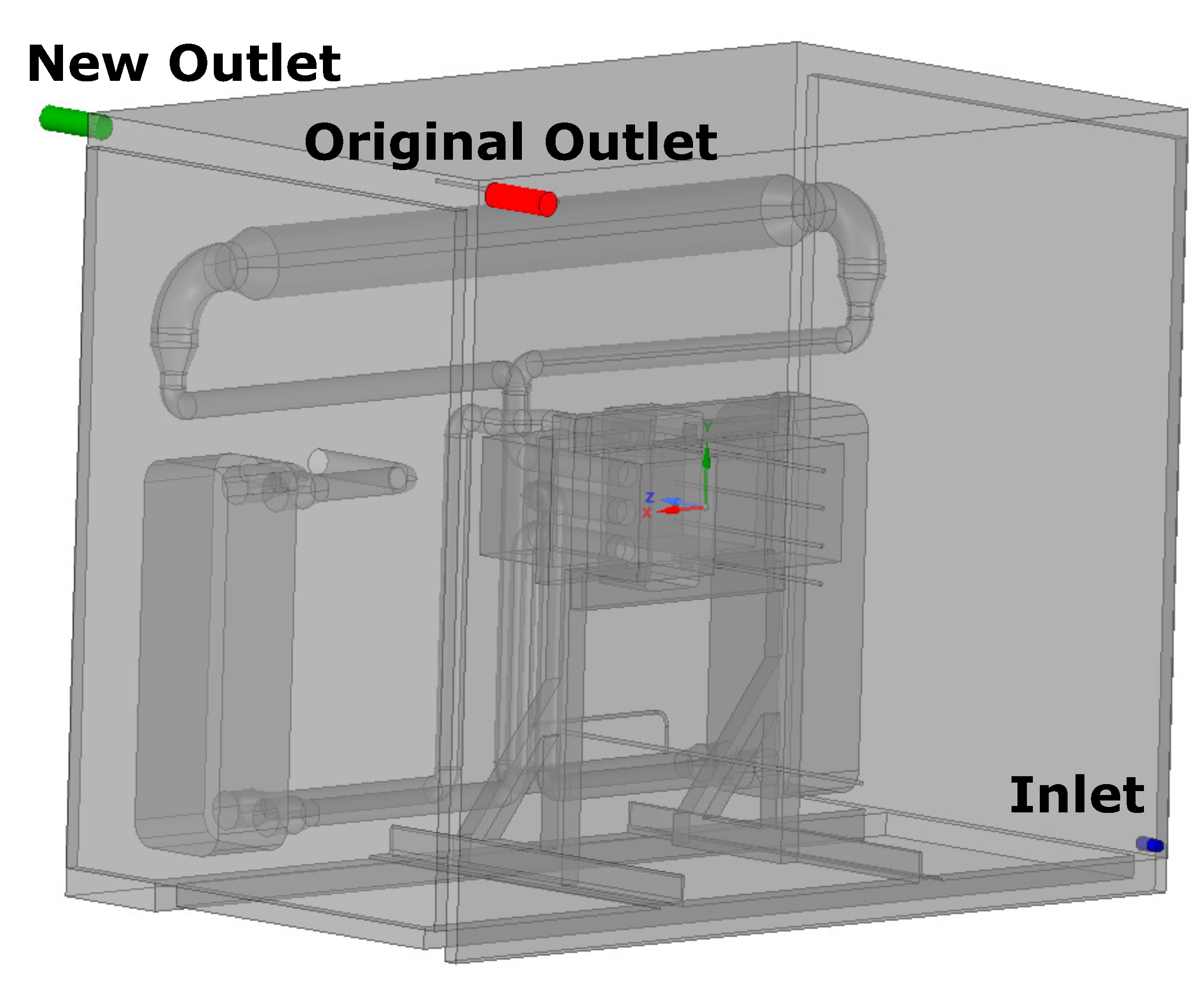
3.4. Alternate Outlet

Figure 14 shows x O 2 , max and x ¯ O 2 for the original outlet and the new outlet, using the SST k ω turbulence model, when T HB , initial = 1073 K. Figure 15 shows x O 2 , max and x ¯ O 2 for the original outlet and the new outlet, using the SST k ω turbulence model when T hot box , initial = 300 K. For the new outlet, x O 2 , max < 0.05 when t / T purge > 0.795 , and this occurs in the original outlet when t / T purge > 0.582 . This means the original is 36.6% faster and needs 36.6% less nitrogen.
Finally, a leakage during the OCV test was also simulated for the new outlet. Figure 16 shows x H 2 , out , max and x ¯ H 2 , out for the original outlet and the new outlet, using the standard k ε turbulence model. The new outlet can detect the leakage after 1.94 < t < 1.95 s. This is 1.2 s faster and corresponds to 62.7% of the original time.

4. Conclusions

  • Based on this study, the initial purge of the hot box, when it is still cold, should last a minimum of t / T purge > 1.58 (94.8 s), corresponding to 3.0 kg of nitrogen. If the outlet is moved to the opposite side, the minimum initial purge period is t / T purge > 1.59 (95.5 s), meaning the effect is negligible.
  • If the hot box is filled with air at T = 1073 K, the hot box should be purged for t / T purge > 0.58 (35 s), corresponding to 1.1 kg of nitrogen. Moving the outlet to the opposite side would increase this period to 48 s. This means the original position is 37% more effective at purging compared to the new position.
  • The leak at the original outlet would take 3.2 s to be detected if the leak was to occur during an OCV test. Moving the outlet to the opposite side would result in a reduction in the detection time by 1.2 s, meaning it is 39% faster.
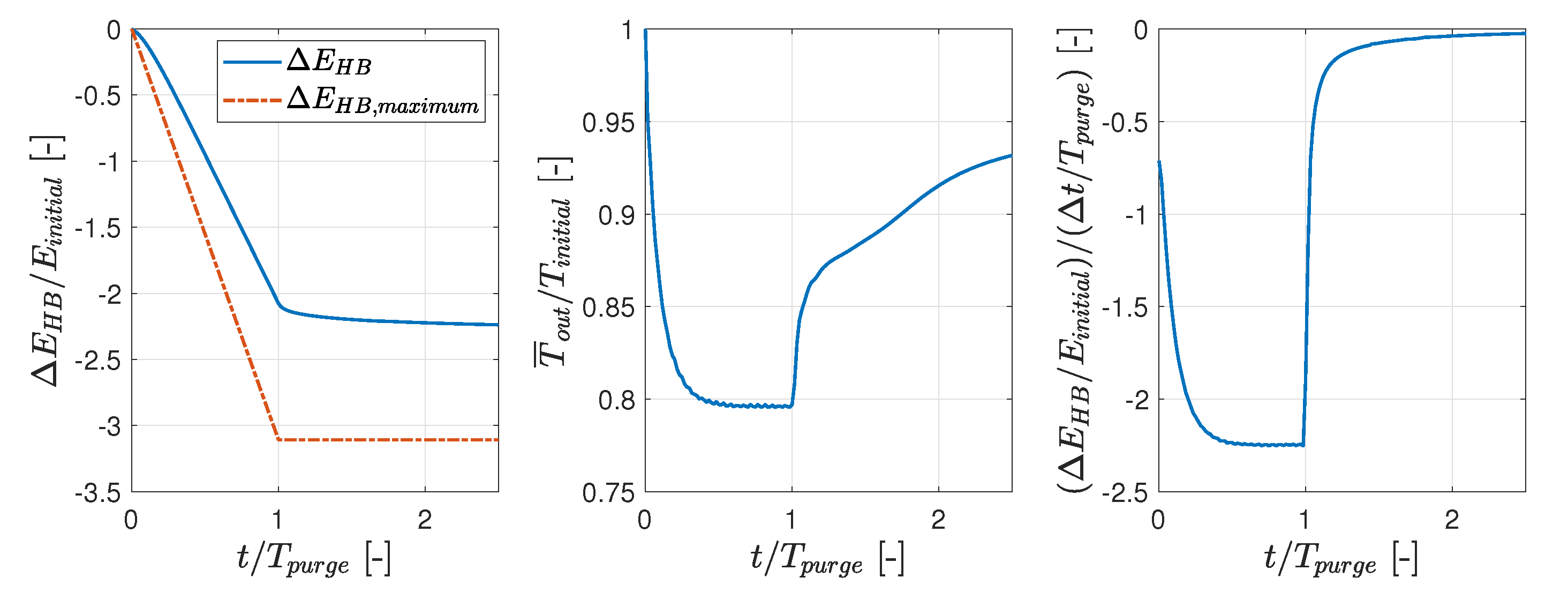
  • During periodic purges of the hot box, while it is operating, it can be expected that 72% of the purging nitrogen is heated from T = 300 K to T = 1073 K. During the purge, the average heat loss is 17.9 kW.
The simulations in this work have not been validated or compared to experimental data. Data acquisition for this type of problem is difficult due to the high temperature of the hot box. Moreover, the test setup was not available during this project. The simulation could also be compared to existing data from similar setups. Nonetheless, the modelling procedure was based on the same methods as used in the literature. Similar detection times were also found in other hydrogen leak simulations [9].

Author Contributions

Conceptualization, R.D.S. and T.B.; methodology, R.D.S. and T.B.; software, R.D.S.; formal analysis, R.D.S.; writing—original draft preparation, R.D.S.; writing—review and editing, T.B.; supervision, T.B. All authors have read and agreed to the published version of the manuscript.

Funding

This research received no external funding.

Data Availability Statement

The data presented in this study are openly available in article.

Acknowledgments

This work was conducted during an internship of RDS at Alfa Laval, Aalborg. The authors want to thank Kasper Gram Bilde at Alfa Laval for the internal supervision and helpful discussions.

Conflicts of Interest

The authors declare no conflict of interest.

Abbreviations

The following abbreviations are used in this manuscript:
CADComputer Aided Design
CFDComputational Fluid Dynamics
FCFuel Cell
HBHot Box
IMOInternational Maritime Organization
LELLower Exlosive Level
LFLLower Flammable Level
LOCLower Oxygen Concentration
OCVOpen Circuit Voltage
RANSReynolds-averaged Navier-Stokes
SOFCSolid Oxide Fuel Cell
SSTShear Stress Transport

References

  1. EU. Europe’s 2030 Climate and Energy Targets: Research & Innovation Actions; Technical Report; European Commission, Directorate-General for Research and Innovation: Brussels, Belgium, 2021. [Google Scholar]
  2. UNFCCC. Adoption of the Paris Agreement. In Proceedings of the 21st Conference of the Parties, United Nations/Framework Convention on Climate Change, Paris, France, 30 November–12 December 2015. [Google Scholar]
  3. IMO. IMO 2020—Cutting Sulphur Oxide Emissions; Technical Report; International Maritime Organization: London, UK, 2020. [Google Scholar]
  4. O’Hayre, R.; Cha, S.W.; Colella, W.; Prinz, F.B. Fuel Cell Fundamentals; John Wiley & Sons: Hoboken, NJ, USA, 2016. [Google Scholar] [CrossRef]
  5. Liso, V.; Xie, P.; Araya, S.S.; Guerrero, J.M. Modelling a modular configuration of PEM fuel cell system for vessels applications. In Proceedings of the 7th World Maritime Technology Conference, Copenhagen, Denmark, 26–28 April 2022; pp. 226–234. [Google Scholar]
  6. Araya, S.S.; Liso, V.; Cui, X.; Li, N.; Zhu, J.; Sahlin, S.L.; Jensen, S.H.; Nielsen, M.P.; Kær, S.K. A Review of The Methanol Economy: The Fuel Cell Route. Energies 2020, 13, 596. [Google Scholar] [CrossRef]
  7. Hagen, A.; Langnickel, H.; Sun, X. Operation of solid oxide fuel cells with alternative hydrogen carriers. Int. J. Hydrogen Energy 2019, 44, 18382–18392. [Google Scholar] [CrossRef]
  8. ABS; CE-DELFT; ARCSILEA. Potential of Ammonia as Fuel in Shipping; Technical report; European Maritime Safety Agency: Lisbon, Portugal, 2022. [Google Scholar]
  9. Heitsch, M.; Baraldi, D.; Moretto, P. Numerical analysis of accidental hydrogen release in a laboratory. Int. J. Hydrog. Energy 2010, 35, 4409–4419. [Google Scholar] [CrossRef]
  10. Dadashzadeh, M.; Ahmad, A.; Khan, F. Dispersion modelling and analysis of hydrogen fuel gas released in an enclosed area: A CFD-based approach. Fuel 2016, 184, 192–201. [Google Scholar] [CrossRef]
  11. Malakhov, A.A.; Avdeenkov, A.V.; du Toit, M.H.; Bessarabov, D.G. CFD simulation and experimental study of a hydrogen leak in a semi-closed space with the purpose of risk mitigation. Int. J. Hydrogen Energy 2020, 45, 9231–9240. [Google Scholar] [CrossRef]
  12. Cinti, G.; Barelli, L.; Bidini, G. The use of ammonia as a fuel for transport: Integration with solid oxide fuel cells. In Proceedings of the 74th ATI NATIONAL CONGRESS: Energy Conversion: Research, Innovation and Development for Industry and Territories, Modena, Italy, 11–13 September 2019. [Google Scholar] [CrossRef]
  13. Molkov, V. Fundamentals of Hydrogen Safety Engineering I; Bookboon: Copenhagen, Denmark, 2012. [Google Scholar]
  14. Kayfeci, M.; Kecebas, A.; Bayat, M. Solar Hydrogen Production, 1st ed.; Academic Press: Cambridge, MA, USA, 2019; pp. 45–83. [Google Scholar]
  15. Kikukawa, S. Consequence analysis and safety verification of hydrogen fueling stations using CFD simulation. Int. J. Hydrogen Energy 2008, 33, 1425–1434. [Google Scholar] [CrossRef]
  16. Bédard-Tremblay, L.; Fang, L.; Melguizo-Gavilanes, J.; Bauwens, L.; Finstad, P.; Cheng, Z.; Tchouvelev, A. Simulation of detonation after an accidental hydrogen release in enclosed environments. Int. J. Hydrogen Energy 2009, 34, 5894–5901. [Google Scholar] [CrossRef]
  17. Mack, A.; Spruijt, M.P. Validation of OpenFoam for heavy gas dispersion applications. J. Hazard. Mater. 2013, 262, 504–516. [Google Scholar] [CrossRef] [PubMed]
  18. Fiates, J.; Vianna, S.S. Numerical modelling of gas dispersion using OpenFOAM. Process. Saf. Environ. Prot. 2016, 104, 277–293. [Google Scholar] [CrossRef]
  19. Yang, Q.; Zhao, P.; Ge, H. reactingFoam-SCI: An open source CFD platform for reacting flow simulation. Comput. Fluids 2019, 190, 114–127. [Google Scholar] [CrossRef]
  20. Versteeg, H.K.; Malalasekera, W. An Introduction to Computational Fluid Dynamics the Finite Volume Method, 2nd ed.; Pearson Education Limited: London, UK, 2007. [Google Scholar]
  21. Gualtieri, C.; Angeloudis, A.; Bombardelli, F.; Jha, S.; Stoesser, T. On the values for the turbulent schmidt number in environmental flows. Fluids 2017, 2, 17. [Google Scholar] [CrossRef]
  22. Greenshields, C. OpenFOAM v10 User Guide; The OpenFOAM Foundation: London, UK, 2022. [Google Scholar]
  23. Laurence, D.R.; Uribe, J.C.; Utyuzhnikov, S.V. A Robust Formulation of the v2-f Model. Flow Turbul. Combust. 2004, 73, 169–185. [Google Scholar] [CrossRef]
  24. Greenshields, C.; Weller, H. Notes on Computational Fluid Dynamics: General Principles; CFD Direct Ltd.: Reading, UK, 2022; p. 291. [Google Scholar]
Figure 1. Production pathways for green ammonia [8].
Hydrogen 04 00054 g001
Figure 2. CAD drawing of the hot box investigated in this study.
Hydrogen 04 00054 g002
Figure 3. Hot box with a hydrogen leak. The left figure is from the front and the right is zoomed in on the back. The hole diameter is 46.7 mm.
Hydrogen 04 00054 g003
Figure 4. The hot box with a relocated outlet. The new outlet is marked in green, the original in red and the inlet in blue. The inlet has a diameter of 18.5 mm.
Hydrogen 04 00054 g004
Figure 5. Maximum molar oxygen fraction during the purge. The red dotted line represents the LOC.
Hydrogen 04 00054 g005
Figure 6. Histogram with x O 2 on the x-axis and probability on the y-axis. Bar width is 0.0005. Top left is at time t / T purge = 0.25 , top right is t / T purge = 0.5 , bottom left is t / T purge = 1 and bottom right is in the steady state.
Hydrogen 04 00054 g006
Figure 7. Molar fraction of oxygen at different time stamps in the hot box, with a threshold above 0.05, for the simulation using the standard k ε model.
Hydrogen 04 00054 g007
Figure 8. The left figure is the normalised energy of the system. The middle figure is the normalised mean outlet temperature. The right figure is the normalised gradient of the energy in the hot box.
Hydrogen 04 00054 g008
Figure 9. The temperature distribution in the hot box at t / T purge = 0.083 and t / T purge = 1.0 . The temperature scales are fixed to 0.79 < T / T H B , i n i t i a l < 0.93 and 0.65 < T / T H B , i n i t i a l < 0.84 , respectively, to better visualise the distribution.
Hydrogen 04 00054 g009
Figure 10. The mean and maximum molar oxygen fraction during the purge. The red dotted line represents the LOC at x O 2 = 5 % . The standard k ε model uses S c lam = 0.76 and S c turb = 0.9 instead of S c = 1 .
Hydrogen 04 00054 g010
Figure 11. Molar oxygen fraction at different time steps in the hot box, with a threshold above 0.05%, for the simulation using the SST k ω model.
Hydrogen 04 00054 g011
Figure 12. The mean and maximum molar hydrogen fraction at the outlet in the time period 0 < t < 16 s. The results are displayed for the three turbulence models, a laminar model and an unmodified k ε model. The red dotted line is the minimum concentration for the sensor to detect hydrogen and the red line is when the sensor will give sound an alarm.
Hydrogen 04 00054 g012
Figure 13. Distribution of hydrogen in the hot box, with a threshold of x H 2 > 0.04 . The top left figure is at t = 2 s, top right is at t = 4 s, bottom left is at t = 8 s and bottom right is at t = 16 s.
Hydrogen 04 00054 g013
Figure 14. Mean and max molar concentration of oxygen for the new and original outlet vs. normalised time for T HB , initial = 1073 K.
Hydrogen 04 00054 g014
Figure 15. Mean and max molar concentration of oxygen for the new and original outlet vs. normalised time for T HB , initial = 300 K.
Hydrogen 04 00054 g015
Figure 16. Mean and max molar concentration of hydrogen at the outlet for the original and new outlet. The sensors detects at x O 2 > 0.4 % and the LFL is defined as x O 2 = 4 %.
Hydrogen 04 00054 g016
Disclaimer/Publisher’s Note: The statements, opinions and data contained in all publications are solely those of the individual author(s) and contributor(s) and not of MDPI and/or the editor(s). MDPI and/or the editor(s) disclaim responsibility for any injury to people or property resulting from any ideas, methods, instructions or products referred to in the content.

