
Spectral Patterns of Pixels and Objects of the Forest Phytophysiognomies in the Anauá National Forest, Roraima State, Brazil

 ,
,  ,
,
Abstract
:1. Introduction
2. Materials and Methods
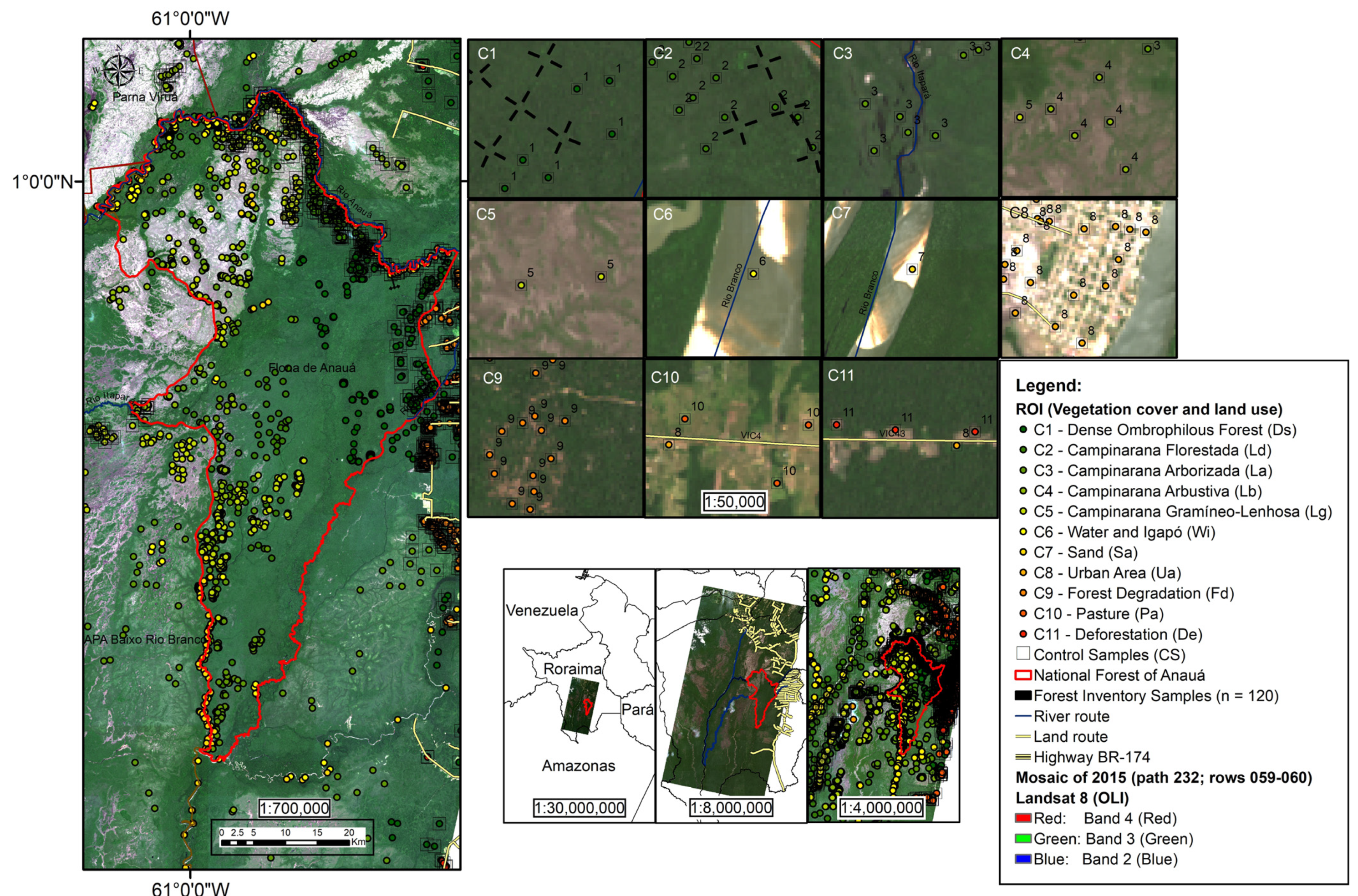
2.1. Study Area and Data Collection
2.2. Data Analysis and Digital Image Processing
2.3. The Spectral Behavior of the Vegetation Indices and Fractional Coverage Image Index
2.4. Pixel-Based Supervised Classification
2.5. Supervised Classification of Geographic Object-Based Image Analysis (GEOBIA)
3. Results
3.1. Vegetation Spectral Patterns
3.2. The Spectral and Spatial Behaviors of the Vegetation Indices and Fractional Coverage Images
3.3. Accuracy Assessment
4. Discussion
5. Conclusions
Supplementary Materials
Author Contributions
Funding
Institutional Review Board Statement
Informed Consent Statement
Data Availability Statement
Acknowledgments
Conflicts of Interest
References
- Bolstad, P.V.; Lillesand, T.M. Rapid Maximum Likelihood Classification. Phot. Eng. Rem. Sens. 1991, 57, 67–74. [Google Scholar]
- Richards, J.A.; Jia, X. Rem. Sens. Digital Image Analysis—An Introduction, 4th ed.; Springer: Berlin/Heidelberg, Germany, 2006. [Google Scholar]
- Benz, U.C.; Hofmann, P.; Willhauck, G.; Lingenfelder, I.; Heynen, M. Multi-resolution, object-oriented fuzzy analysis of remote sensing data for GIS-ready information. ISPRS J. Phot. Rem. Sens. 2004, 58, 239–258. [Google Scholar] [CrossRef]
- Walter, V. Object-based classification of remote sensing data for change detection. ISPRS J. Phot. Rem. Sens. 2004, 58, 225–238. [Google Scholar] [CrossRef]
- Chubey, M.S.; Franklin, S.E.; Wulder, M.A. Object-based Analysis of Ikonos-2 Imagery for Extraction of Forest Inventory Parameters. Phot. Eng. Rem. Sens. 2006, 72, 383–394. [Google Scholar] [CrossRef]
- Bontemps, S.; Bogaert, P.; Titeux, N.; Defourny, P. An object-based change detection method accounting for temporal dependences in time series with medium to coarse spatial resolution. Remote Sens. Environ. 2008, 112, 3181–3191. [Google Scholar] [CrossRef]
- Blaschke, T. Object based image analysis for remote sensing. ISPRS J. Photo. Remote Sens. 2010, 65, 2–16. [Google Scholar] [CrossRef]
- Lyons, M.B.; Roelfsema, C.M.; Phinn, S.R. Towards understanding temporal and spatial dynamics of seagrass landscapes using time-series remote sensing. Est., Coast. Shelf Sci. 2013, 120, 42–53. [Google Scholar] [CrossRef]
- Hay, G.J.; Castilla, G. Geographic Object-Based Image Analysis (GEOBIA): A new name for a new discipline. In Object-Based Image Analysis, Lecture Notes in Geoinformation and Cartography; Blaschke, T., Lang, S., Hay, G.J., Eds.; Springer: Berlin/Heidelberg, Germany, 2008; pp. 75–89. [Google Scholar] [CrossRef]
- Blaschke, T.; Hay, G.J.; Kelly, M.; Lang, S.; Hofmann, P.; Addink, E.; Feitosa, R.Q.; van der Meer, F.; van der Werff, H.; van Coillie, F.; et al. Geographic Object-Based Image Analysis—Towards a new paradigm. ISPRS J. Photo. Remote Sens. 2014, 87, 180–191. [Google Scholar] [CrossRef]
- Watmough, G.R.; Palm, C.A.; Sullivan, C. An operational framework for object-based land use classification of heterogeneous rural landscapes. Int. J. Appl. Earth Observ. Geoinform. 2017, 54, 134–144. [Google Scholar] [CrossRef]
- Fisher, P. The pixel: A snare and a delusion. Inter. J. Remote Sens. 1997, 18, 679–685. [Google Scholar] [CrossRef]
- Blaschke, T.; Strobl, J. What’s Wrong with Pixels? Some Recent Developments Interfacing Remote Sensing and GIS. Z. Fur Geoinf. Syst. 2001, 14, 12–17. [Google Scholar]
- Kelly, M.; Blanchard, S.D.; Kersten, E.; Koy, K. Terrestrial Remotely Sensed Imagery in Support of Public Health: New Avenues of Research Using Object-Based Image Analysis. Rem. Sens. 2011, 3, 2321–2345. [Google Scholar] [CrossRef]
- Pereira, R., Jr.; Zweede, J.; Asner, G.P.; Keller, M. Forest canopy damage and recovery in reduced-impact and conventional selective logging in eastern Para, Brazil. For. Ecol. Manag. 2002, 168, 77–89. [Google Scholar] [CrossRef]
- Asner, G.P.; Knapp, D.E.; Broadbent, E.N.; Oliveira, P.J.C.; Keller, M.; Silva, J.N.M. Selective Logging in the Brazilian Amazon. Science 2005, 310, 480–482. [Google Scholar] [CrossRef] [PubMed]
- Asner, G.P.; Knapp, D.E.; Balaji, A.; Paez-Acosta, G. Automated mapping of tropical deforestation and forest degradation: CLASlite. J. Appl. Remote Sens. 2009, 3, 033543. [Google Scholar] [CrossRef]
- Condé, T.M.; Higuchi, N.; Lima, A.J.N. Illegal selective logging and forest fires in the Northern Brazilian Amazon. Forests 2019, 10, 61. [Google Scholar] [CrossRef]
- Higuchi, N.; Santos, J.; Ribeiro, R.J.; Minette, L.; Biot, Y. Biomassa da Parte Aérea da Vegetação da Floresta Tropical Úmida de Terra-firme da Amazônia Brasileira. Acta Amazon. 1998, 28, 153–166. [Google Scholar] [CrossRef]
- Fearnside, P.M.; Barbosa, R.I.; Pereira, V.B. Emissões de gases do efeito estufa por desmatamento e incêndios florestais em Roraima: Fontes e sumidouros. Agro@Mbiente 2013, 7, 95–111. [Google Scholar] [CrossRef]
- Ichoku, C.; Karnieli, A. A review of mixture modeling techniques for sub-pixel land cover estimation. Rem. Sens. Rev. 1996, 13, 161–186. [Google Scholar] [CrossRef]
- Jensen, J.R. Sensoriamento Remoto do Ambiente: Uma Perspectiva em Recursos Terrestres, 2nd ed.; Prentice Hall Series in Geographic Information Science/Parêntesis: São Paulo, Brazil, 2009. [Google Scholar]
- James, G.; Witten, D.; Hastie, T.; Tibshirani, R. An Introduction to Statistical Learning with Applications in R, 1st ed.; Springer: New York, NY, USA, 2013. [Google Scholar]
- Durgante, F.M.; Higuchi, N.; Almeida, A.; Vicentini, A. Species Spectral Signature: Discriminating closely related plant species in the Amazon with Near-Infrared Leaf-Spectroscopy. For. Ecol. Manag. 2013, 291, 240–248. [Google Scholar] [CrossRef]
- Carter, G.A.; Knapp, A.K. Leaf optical properties in higher plants: Linking spectral characteristics to stress and chlorophyll concentration. Am. J. Bot. 2001, 88, 677–684. [Google Scholar] [CrossRef] [PubMed]
- Ponzoni, F.J.; Resende, A.C.P. Caracterização espectral de estágios sucessionais de vegetação secundária arbórea em Altamira (PA), através de dados orbitais. R. Árvore 2004, 28, 535–545. [Google Scholar] [CrossRef]
- Hopkins, M.J.G. Modelling the known and unknown plant biodiversity of the Amazon Basin. J. Biogeog. 2007, 34, 1400–1411. [Google Scholar] [CrossRef]
- Condé, T.M.; Tonini, H. Fitossociologia de uma Floresta Ombrófila Densa na Amazônia Setentrional, Roraima, Brasil. Acta Amaz. 2013, 43, 247–260. [Google Scholar] [CrossRef]
- Adeney, J.M.; Christensen, N.L.; Vicentini, A.; Cohn-Haft, M. White-sand Ecosystems in Amazonia. Biotropica 2016, 48, 7–23. [Google Scholar] [CrossRef]
- Guevara, J.E.; Damasco, G.; Baraloto, C.; Fine, P.V.A.; Peñuela, M.C.; Castilho, V.C.; Vincentini, A.; Cárdenas, D.; Wittmann, F.; Targhetta, N.; et al. Low Phylogenetic Beta Diversity and Geographic Neo-endemism in Amazonian White-sand Forests. Biotropica 2016, 48, 34–46. [Google Scholar] [CrossRef]
- Anderson, A.B. White-sand vegetation of Brazilian Amazonia. Biotropica 1981, 13, 199–210. [Google Scholar] [CrossRef]
- Mendonça, B.A.F.; Filho, E.I.F.; Schaefer, C.E.G.R.; Simas, F.N.B.; Paula, M.D. The soils of “Campinaranas” in Brazilian Amazon: Oligothrophic Sandy Ecosystems. Ciência Florest. 2015, 25, 827–839. [Google Scholar] [CrossRef]
- Asner, G.P.; Townsend, A.R.; Bustamante§, M.M.C.; Nardoto, G.B.; Olander, L.P. Pasture degradation in the central Amazon: Linking changes in carbon and nutrient cycling with remote sensing. Glob. Change Biol. 2004, 10, 844–862. [Google Scholar] [CrossRef]
- Nepstad, D.; McGrath, D.; Stickler, C.; Alencar, A.; Azevedo, A.; Swette, B.; Bezerra, T.; DiGiano, M.; Shimada, J.; Motta, R.S.; et al. Slowing Amazon deforestation through public policy and interventions in beef and soy supply chains. Science 2014, 344, 1118–1124. [Google Scholar] [CrossRef]
- Dionisio, L.F.S.; Condé, T.M.; Gomes, J.P.; Martins, W.B.R.; Silva, M.W.; Silva, M.T. Caracterização morfométrica de árvores solitárias de Bertholletia excelsa H.B.K. no sudeste de Roraima. Rev. Agro@Mbiente Line 2017, 11, 163–173. [Google Scholar] [CrossRef]
- ICMBio. Chico Mendes Institute of Biodiversity. PAN Portaria n° 457. Plano de Manejo da Floresta Nacional de Anauá. 2022. Available online: https://www.gov.br/icmbio/pt-br/assuntos/biodiversidade/unidade-de-conservacao/unidades-de-biomas/amazonia/lista-de-ucs/flona-de-anaua/arquivos/pm_flona_anaua_consolidado_vs-10.pdf (accessed on 27 September 2023).
- IBGE. Brazilian Institute of Geography and Statistics. Manual Técnico da Vegetação Brasileira. Available online: https://biblioteca.ibge.gov.br/index.php/biblioteca-catalogo?view=detalhes&id=263011 (accessed on 1 March 2023).
- ICMBio. Chico Mendes Institute of Biodiversity. PAN Sirênios. Plano de Ação Nacional para a Conservação dos Sirênios Peixe-boi-da-Amazônia (Trichechus inunguis) e Peixe-Boi Marinho (Trichechus manatus manatus). 2011. Available online: https://www.gov.br/icmbio/pt-br/assuntos/biodiversidade/pan/pan-sirenios/1-ciclo/pan-sirenios-livro.pdf (accessed on 1 February 2023).
- USGS. United States Geological Survey. Landsat Missions Timeline—Landsat 8. Available online: https://landsat.usgs.gov/landsat-8-history (accessed on 2 July 2017).
- R Development Core Team. R: A Language and Environment for Statistical Computing. Available online: http://www.R-project.org (accessed on 1 July 2022).
- Gao, B.C. NDWI—A normalized difference water index for remote sensing of vegetation liquid water from space. Rem. Sens. Environ. 1996, 58, 257–266. [Google Scholar] [CrossRef]
- Jin, S.; Sader, S.A. MODIS time-series imagery for forest disturbance detection and quantification of patch size effects. Remote Sens. Environ. 2005, 99, 462–470. [Google Scholar] [CrossRef]
- Landis, J.R.; Koch, G.G. The Measurement of Observer Agreement for Categorical Data. Biometrics 1977, 33, 159–174. [Google Scholar] [CrossRef] [PubMed]
- Haralick, R.M.; Shanmugam, K.; Dinstein, I. Textural Features for Image Classification. IEEE Trans. Syst. Man Cybernet. 1973, 6, 610–621. [Google Scholar] [CrossRef]
- Gates, D.M.; Keegan, H.J.; Schleter, J.C.; Weidner, V.R. Spectral properties of plants. Appl. Opt. 1965, 4, 11–20. [Google Scholar] [CrossRef]
- Rock, B.N.; Vogelmann, J.E.; Williams, D.L.; Vogelmann, A.F.; Hoshizaki, T. Remote Detection of Forest Damage: Plant responses to stress may have spectral “signatures” that could be used to map, monitor, and measure forest damage. BioScience 1986, 36, 439–445. [Google Scholar] [CrossRef]
- Kodani, E.; Awaya, Y.; Tanaka, K.; Matsumura, N. Seasonal patterns of canopy structure, biochemistry and spectral reflectance in a broad-leaved deciduous Fagus crenata canopy. For. Ecol. Manag. 2002, 167, 233–249. [Google Scholar] [CrossRef]
- Asner, G.P.; Martin, R.E.; Knapp, D.E.; Tupayachi, R.; Anderson, C.; Carranza, L.; Martinez, P.; Houcheime, M.; Sinca, F.; Weiss, P. Spectroscopy of canopy chemicals in humid tropical forests. Rem. Sens. Environ. 2011, 115, 3587–3598. [Google Scholar] [CrossRef]
- Blackburn, G.A. Hyperspectral remote sensing of plant pigments. J. Exp. Bot. 2007, 58, 855–867. [Google Scholar] [CrossRef]
- Asner, G.P.; Martin, R.E. Airborne spectranomics: Mapping canopy chemical and taxonomic diversity in tropical forests. Front. Ecol. Environ. 2008, 7, 269–276. [Google Scholar] [CrossRef]
- Asner, G.P.; Martin, R.E.; Carranza-Jiménez, L.; Sinca, F.; Tupayachi, R.; CMartinez, P. Functional and biological diversity of foliar spectra in tree canopies throughout the Andes to Amazon region. New Phytol. 2014, 204, 127–139. [Google Scholar] [CrossRef]
- Davidson, E.A.; Araújo, A.C.; Artaxo, P.; Balch, J.K.; Brown, I.F.; Bustamante, M.M.C.; Coe, M.T.; DeFries, R.S.; Keller, M.; Longo, M.; et al. The Amazon basin in transition. Nature 2012, 481, 321–328. [Google Scholar] [CrossRef] [PubMed]
- Condé, T.M.; Tonini, H.; Higuchi, N.; Higuchi, F.G.; Lima, A.J.N.; Barbosa, R.I.; Pereira, T.S.; Haas, M.A. Effects of sustainable forest management on tree diversity, timber volumes, and carbon stocks in an ecotone forest in the northern Brazilian Amazon. Land Use Policy 2022, 119, 106145. [Google Scholar] [CrossRef]


| Class | Vegetation Cover and Land Use | Initials | Description | Colors |
|---|---|---|---|---|
| ROI | ||||
| C1 | Dense Ombrophilous Forest | Ds | Dense forest cover, high textural roughness, no soil exposure. | |
| C2 | Campinarana Florestada | Ld | Dense forest cover, medium textural roughness, no soil exposure. | |
| C3 | Campinarana Arborizada | La | Environment with trees and shrubs, with slight soil exposure. | |
| C4 | Campinarana Arbustiva | Lb | Environment with shrubs and average soil exposure. | |
| C5 | Campinarana Gramíneo-Lenhosa | Lg | Environment with grasses and high soil exposure. | |
| C6 | Water and Igapó | Wi | Rivers, streams, and flooded environments | |
| C7 | Sand | Sa | Environment with sandy soils. | |
| C8 | Urban area | Ua | Anthropically altered areas with different degrees of urbanization. | |
| C9 | Forest Degradation | Fd | Areas impacted by illegal selective logging. | |
| C10 | Pasture | Pa | Pasture areas in different states of conservation. | |
| C11 | Deforestation | De | Areas with forest cover removed, with soil exposure. |
| Class | Vegetation Cover and Land Use | Spectral Patterns |
|---|---|---|
| C1 |  Dense Ombrophilous Forest (Ds) |  |
| C2 |  Campinarana Florestada (Ld) |  |
| C3 |  Campinarana Arborizada (La) |  |
| C4 |  Campinarana Arbustiva (Lb) |  |
| C5 |  Campinarana Gramíneo-Lenhosa (Lg) |  |
| C6 |  Water and Igapó (Wi) |  |
| C7 |  Sand (Sa) |  |
| C8 |  Urban area (Ua) |  |
| C9 |  Forest Degradation (Fd) |  |
| C10 |  Pasture (Pa) |  |
| C11 |  Deforestation (De) |  |
| Parameters/Bands | Blue | Green | Red | NIR | SWIR 1 or MIR |
|---|---|---|---|---|---|
| Landsat 8 (OLI) | b2 | b3 | b4 | b5 | b6 |
| ROI samples | 4400 | 4400 | 4400 | 4400 | 4400 |
| Minimum | 0.01 | 0.01 | 0.01 | 0.00 | 0.00 |
| Maximum | 0.41 | 0.50 | 0.57 | 0.65 | 0.86 |
| Median | 0.03 | 0.05 | 0.04 | 0.27 | 0.17 |
| Average | 0.04 | 0.06 | 0.06 | 0.26 | 0.19 |
| IC95% Lower | 0.04 | 0.06 | 0.06 | 0.26 | 0.19 |
| IC95% Upper | 0.04 | 0.06 | 0.07 | 0.26 | 0.20 |
| Standard deviation | 0.03 | 0.05 | 0.06 | 0.09 | 0.12 |
| Variance | 0.001 | 0.002 | 0.004 | 0.008 | 0.013 |
| ANOVA | 1122.9 | 1396.2 | 1547.0 | 1394.1 | 1327.0 |
| p-value | 0.000 | 0.000 | 0.000 | 0.000 | 0.000 |
| Blue (0.45–0.51 µm) | Green (0.53–0.59 µm) | Red (0.64–0.67 µm) | NIR (0.85–0.88 µm) | SWIR 1/MIR (1.57–1.65 µm) | |||||||||||||||
|---|---|---|---|---|---|---|---|---|---|---|---|---|---|---|---|---|---|---|---|
| SG | Class | Mean | p | SG | Class | Mean | p | SG | Class | Mean | p | SG | Class | Mean | p | SG | Class | Mean | p |
| 1 | C6 | 0.017 | 1.0 | 1 | C6 | 0.025 | 1.0 | 1 | C6 | 0.022 | 1.0 | 1 | C6 | 0.076 | 1.0 | 1 | C6 | 0.036 | 1.0 |
| C1 | 0.017 | 2 | C1 | 0.037 | 1.0 | C1 | 0.022 | 2 | C5 | 0.170 | 1.0 | 2 | C1 | 0.134 | 1.0 | ||||
| C2 | 0.018 | C2 | 0.040 | C2 | 0.024 | 3 | C4 | 0.212 | 1.0 | C2 | 0.139 | ||||||||
| 2 | C9 | 0.021 | 1.0 | C9 | 0.040 | 2 | C9 | 0.031 | 1.0 | 4 | C11 | 0.223 | 1.0 | C3 | 0.140 | ||||
| 3 | C3 | 0.024 | 1.0 | 3 | C3 | 0.045 | 1.0 | C3 | 0.034 | 5 | C3 | 0.259 | 1.0 | 3 | C9 | 0.154 | 1.0 | ||
| 4 | C4 | 0.031 | 1.0 | C5 | 0.047 | 3 | C4 | 0.047 | 1.0 | 6 | C9 | 0.286 | 1.0 | 4 | C5 | 0.169 | 1.0 | ||
| C5 | 0.033 | C4 | 0.049 | C5 | 0.051 | 7 | C8 | 0.294 | 1.0 | 5 | C4 | 0.179 | 1.0 | ||||||
| 5 | C10 | 0.035 | 1.0 | 4 | C11 | 0.056 | 1.0 | 4 | C11 | 0.064 | 1.0 | 8 | C1 | 0.310 | 1.0 | 6 | C10 | 0.222 | 1.0 |
| C11 | 0.036 | 5 | C10 | 0.073 | 1.0 | C10 | 0.067 | 9 | C2 | 0.318 | 1.0 | 7 | C11 | 0.234 | 1.0 | ||||
| 6 | C8 | 0.070 | 1.0 | 6 | C8 | 0.104 | 1.0 | 5 | C8 | 0.116 | 1.0 | 10 | C10 | 0.337 | 1.0 | 8 | C8 | 0.286 | 1.0 |
| 7 | C7 | 0.117 | 1.0 | 7 | C7 | 0.177 | 1.0 | 6 | C7 | 0.224 | 1.0 | 11 | C7 | 0.367 | 1.0 | 9 | C7 | 0.446 | 1.0 |
| MSE | 0.0003 | MSE | 0.0005 | MSE | 0.0009 | MSE | 0.0020 | MSE | 0.0034 | ||||||||||
| Class | NDVI | NDWI | Fractional Coverage Image (FCI) | ||
|---|---|---|---|---|---|
| BARE (%) | PV (%) | NPV (%) | |||
| C1 | 0.86 ± 0.01 | 0.40 ± 0.02 | 0.97 ± 2.31 | 93.93 ± 2.06 | 8.64 ± 3.75 |
| C2 | 0.86 ± 0.02 | 0.39 ± 0.02 | 2.09 ± 3.39 | 92.28 ± 2.85 | 8.14 ± 4.03 |
| C3 | 0.77 ± 0.03 | 0.30 ± 0.06 | 0.25 ± 1.26 | 85.37 ± 6.62 | 19.33 ± 6.22 |
| C4 | 0.64 ± 0.06 | 0.09 ± 0.09 | 0.04 ± 0.54 | 65.17 ± 13.00 | 46.74 ± 15.07 |
| C5 | 0.53 ± 0.08 | 0.03 ± 0.16 | 0.06 ± 0.58 | 61.42 ± 23.44 | 43.10 ± 22.75 |
| C6 | 0.43 ± 0.31 | 0.36 ± 0.11 | 0.12 ± 0.67 | 22.80 ± 40.12 | 2.87 ± 5.82 |
| C7 | 0.25 ± 0.11 | −0.08 ± 0.11 | 15.43 ± 23.07 | 13.41 ± 23.70 | 29.68 ± 34.16 |
| C8 | 0.45 ± 0.16 | 0.03 ± 0.12 | 16.07 ± 18.64 | 35.47 ± 23.73 | 48.22 ± 21.91 |
| C9 | 0.81 ± 0.06 | 0.30 ± 0.09 | 0.84 ± 2.20 | 85.25 ± 9.95 | 19.17 ± 11.07 |
| C10 | 0.67 ± 0.06 | 0.20 ± 0.10 | 11.00 ± 10.15 | 64.97 ± 11.71 | 24.95 ± 15.99 |
| C11 | 0.55 ± 0.13 | −0.0267 ± 0.12 | 1.01 ± 3.46 | 50.64 ± 16.53 | 54.93 ± 20.81 |
| Class | Maximum Likelihood (Per-Pixel) | GEOBIA | |||||||
|---|---|---|---|---|---|---|---|---|---|
| R(4)G(3)B(2) | (%) | R(5)G(4)B(3) | (%) | R(6)G(5)B(4) | (%) | Anauá National Forest | (%) | Mosaic | |
| (Km2) | (Km2) | (Km2) | (Km2) | (Km2) | |||||
| C1 | 755 | 29 | 712 | 27 | 980 | 27 | 992 | 38 | 26,508 |
| C2 | 1132 | 44 | 1169 | 45 | 898 | 45 | 807 | 31 | 16,560 |
| C3 | 170 | 7 | 207 | 8 | 214 | 8 | 274 | 11 | 9096 |
| C4 | 257 | 10 | 313 | 12 | 285 | 12 | 231 | 9 | 4395 |
| C5 | 141 | 5 | 109 | 4 | 88 | 4 | 201 | 8 | 3451 |
| C6 | 6 | 0 | 9 | 0 | 14 | 0 | 11 | 0 | 37,328 |
| C7 | 2 | 0 | 2 | 0 | 3 | 0 | 26 | 1 | 1283 |
| C8 | 10 | 0 | 5 | 0 | 3 | 0 | 8 | 0 | 501 |
| C9 | 76 | 3 | 22 | 1 | 33 | 1 | 34 | 1 | 2439 |
| C10 | 1 | 0 | 3 | 0 | 3 | 0 | 0 | 0 | 614 |
| C11 | 45 | 2 | 45 | 2 | 75 | 2 | 0 | 0 | 30 |
| Total | 2596 | 100 | 2596 | 100 | 2596 | 100 | 2584 | 100 | 102,204 |
Disclaimer/Publisher’s Note: The statements, opinions and data contained in all publications are solely those of the individual author(s) and contributor(s) and not of MDPI and/or the editor(s). MDPI and/or the editor(s) disclaim responsibility for any injury to people or property resulting from any ideas, methods, instructions or products referred to in the content. |
© 2023 by the authors. Licensee MDPI, Basel, Switzerland. This article is an open access article distributed under the terms and conditions of the Creative Commons Attribution (CC BY) license (https://creativecommons.org/licenses/by/4.0/).
Share and Cite
Condé, T.M.; Higuchi, N.; Lima, A.J.N.; Campos, M.A.A.; Condé, J.D.; de Oliveira, A.C.; de Miranda, D.L.C. Spectral Patterns of Pixels and Objects of the Forest Phytophysiognomies in the Anauá National Forest, Roraima State, Brazil. Ecologies 2023, 4, 686-703. https://doi.org/10.3390/ecologies4040045
Condé TM, Higuchi N, Lima AJN, Campos MAA, Condé JD, de Oliveira AC, de Miranda DLC. Spectral Patterns of Pixels and Objects of the Forest Phytophysiognomies in the Anauá National Forest, Roraima State, Brazil. Ecologies. 2023; 4(4):686-703. https://doi.org/10.3390/ecologies4040045
Chicago/Turabian StyleCondé, Tiago Monteiro, Niro Higuchi, Adriano José Nogueira Lima, Moacir Alberto Assis Campos, Jackelin Dias Condé, André Camargo de Oliveira, and Dirceu Lucio Carneiro de Miranda. 2023. "Spectral Patterns of Pixels and Objects of the Forest Phytophysiognomies in the Anauá National Forest, Roraima State, Brazil" Ecologies 4, no. 4: 686-703. https://doi.org/10.3390/ecologies4040045