Article

Investigating the Impact of Undulation Amplitude of Unconventional Oil Well Laterals on Transient Multiphase Flow Behavior: Experimental and Numerical Study

Department of Petroleum Engineering, College of Engineering and Mines, University of North Dakota, Upson II Room 165, 243 Centennial Dr Stop 8155, Grand Forks, ND 58202, USA
*
Author to whom correspondence should be addressed.
Fuels 2023, 4(4), 417-440; https://doi.org/10.3390/fuels4040026
Submission received: 19 June 2023 / Revised: 31 August 2023 / Accepted: 29 September 2023 / Published: 24 October 2023

Abstract

:
The growing popularity of unconventional wells has led to increased interest in assessing and predicting their production performance. These wells, with their extended-reach structures, are able to generate and access larger reservoir volumes. Therefore, understanding the impact of a well’s lateral trajectory on its transient production performance is crucial. This study investigates the effect of lateral-trajectory undulation amplitude on flow behavior based on the experimental results obtained at the University of North Dakota using an undulated two-phase (UTP) flow loop. The experiments involved injecting an air-and-water mixture through a section with variable undulation amplitude followed by a vertical section. The results revealed that the increasing undulation amplitude resulted in lower translational velocity, frequency, and length, with consistent slug acceleration along the system profile. Additionally, the frequency of slugs decreased as they traveled through the vertical section. The measured data indicated that higher undulation amplitudes led to increased horizontal pressure losses and variability, suggesting larger instabilities. The numerical simulations predicted lower translational velocity and frequency, longer slug length, and similar vertical pressure losses when compared to the experimental results.

Graphical Abstract

1. Introduction

Horizontal-well technology plays a crucial role in extracting unconventional resources, particularly in tight oil- and gas-rich formations like the Bakken and Three Forks formations in the Williston Basin. Implementing multistage hydraulic fracturing along the lateral section of these wells enhances production. Research conducted by [1] demonstrates that optimal production from these formations can be achieved with horizontal wells having a measured-to-vertical depth ratio of two or higher. Horizontal liquid-producing wells face flow stability challenges that seem inherent to their structure, as highlighted in [2]. Severe slugging leads to high-pressure oscillations downhole along the lateral section, impacting the integrity of the hydraulic fractures, as demonstrated in [3], and potentially causing proppant displacement and fracture closure due to excessive drawdown, as shown in [4].
Slugging is an undesired phenomenon creating flow instabilities, which can impair the performance of liquid-producing wells, as shown in [1,5,6], which also has implications for gas-well liquid-loading studies, as shown in [7,8,9,10,11,12,13,14], and CO2 storage due to wellbore phase change, as shown in [15,16,17,18,19,20,21].
Few studies have examined the impact of well-trajectory undulations on flow characteristics. In one study [22], a transient multiphase flow simulation model showed that trajectory effects are significant only at low production rates, particularly with toe-up geometries resulting in the highest cumulative production in high-productivity and toe-down geometries resulting in the highest cumulative production in the low-productivity case, with the first geometry being the most unstable. However, this study only explored five undulations without definitive findings. Another study [23] investigated the toe-up trajectory under different flow conditions (gas lift, packerless, and variable end-of-tubing depth) without a specific focus on lateral-trajectory undulation. Similarly, Ref. [24] addressed the differences in well-trajectory performance for various artificial lift techniques but did not focus on trajectory undulation.
An experimental study in [25] examined the effect of trajectory and end-of-tubing depth optimization on flow behavior and found that the toe-down trajectory can prevent severe slugging under certain flow conditions. However, this study did not investigate the impact of lateral-trajectory undulation parameters on flow behavior.
In contrast, in [5], a comprehensive statistical analysis was conducted using basin-wide field data, synthetic and realistic transient numerical simulation, and flow-loop experimental tests. The authors captured the undulation amplitude’s effect on pressure oscillations and slug characteristics in their experimental system. However, they only briefly described pressure variability, horizontal and vertical loss profile distribution, and flow-condition averaged data. The present study, on the other hand, specifically focuses on these aspects of the experimental data and provides new insights, as described in the conclusions.
Based on the above critical literature review, it is clear that flow instabilities are crucial to evaluating horizontal oil well production performance. Factors influencing flow instabilities and oscillations are of significant interest for further understanding the topic, and the transient flow behavior depends on the fluid properties, flow conditions, and system structure. This study specifically examines how well-trajectory characteristics impact the transient behavior of horizontal wells. The authors of [26,27,28] showed that the effect of trajectory on the flow regime is not significant at high velocities but becomes more pronounced as velocity decreases, particularly under gravity-dominated flow conditions. This highlights the increasing dominance of the well structure in such scenarios.
The existing literature has explored the impact of well lateral section trajectory on performance, but it has mostly focused on the effects of single undulations rather than considering the impact of the multiple-undulation effect on flow performance, as mentioned in [26]. The fundamental experimental and modeling study reveals that under constant flow conditions, toe-down configurations exhibit liquid film fallback and accumulation at low gas flow rates, whereas toe-up configurations result in a stratified flow regime with no liquid accumulation in the lateral section. However, for very low gas flow rates, severe slugging is observed, leading to high pressure and rate fluctuations. In the case of a single-undulation configuration, the study demonstrates that for moderate gas flow rates, a stratified wavy flow regime is observed. Conversely, at low gas flow rates, slugs form at the lowest undulation point, and slug flow is observed in the upward pipe section with significant liquid accumulation in the lateral section. Moreover, convex (hump) undulations induce higher instabilities compared with concave (sump) undulations. It is important to note that the above study focuses solely on one undulation configuration without considering the effect of undulation amplitude and the presence of multiple undulations. A more practical simulation study, presented in [29], examines the impact of the well geometry with five undulations, with one including a combination of humps, sumps, and toe-up and toe-down configurations, on production performance, particularly at low production rates. The study suggests that toe-up configurations yield optimal productivity in high-productivity cases, while toe-down trajectories perform better in low productivity, reducing the severity of fluctuations.
No literature currently focuses on examining the impact of undulation amplitude on flow behavior. However, it is crucial to understand that higher undulation amplitudes can result in longer flow paths and increased sinuosity, leading to a greater variation in vertical depth along the lateral section. This understanding is essential for studying transient behavior or steadiness, particularly in the context of slugging cyclicity, and analyzing various flow parameters such as three-phase (oil, gas, and water) flow rates, translational velocity, frequency and length of slugs, lateral and vertical pressure losses, and the temporal variability of pressure along the lateral and top vertical sections. These parameters constitute a set of key performance indicators (KPIs) that are used to analyze experimental test data and evaluate the system’s performance.

2. Materials and Methods

The experimental system utilized in this study is an undulated two-phase (UTP) flow loop, specifically designed at the University of North Dakota Petroleum Engineering Department. It comprises a semi-flexible clear 2″ inner diameter pipe with adjustable undulations to control the amplitude. As illustrated in Figure 1, the system includes a water tank serving as a two-phase separator, with the liquid being pumped to the desired test inlet pressure using a centrifugal pump. The liquid flow is accurately measured by a turbine and an ultrasonic flowmeter, which are followed by a control valve and a block valve before entering the mixing tee. The air is compressed by the reciprocating compressor and stored in a compressor tank to ensure a stable air flowrate and prevent interference with the test flow regimes. Prior to entering the mixing tee, the air passes through filters, a pressure regulator, a mass flowmeter, a check valve, and control and block valves. At the mixing tee, a pressure transmitter measures the inlet pressure of the test section, followed by the undulated sections where pressure and water holdup measurements are taken at each inflection point.
A maximum of three undulations can be configured in the system with a total length-to-diameter ratio of L/D = 313. Each piece of equipment, each fitting, and each instrument are labeled physically and electronically using the DAQ National Instruments® data acquisition system. In Figure 1, the instruments and fittings (valves) are highlighted in red to indicate their labeling. It is important to note that the flow loop is equipped with a gas lift feature, although it is not utilized in the present study.
The undulation amplitude is defined as the distance between the horizontal hypothetical line starting at the test section inlet height and the horizontal line formed by the lower inflection points. This is illustrated in Figure 2 for one undulation characteristic and in the overall test section structure in Figure 1. The inclination angle and variation of the undulation amplitude are obtained by adjusting the vertical position of the water-holdup probe and the pressure-sensor tee. By adjusting the vertical position, undulation amplitudes of 0, 5, 10, and 20 cm can be obtained, which correspond to 0, 1, 2, and 4 times the diameter in terms of dimensionless undulation amplitude.
The operation of the experimental facility utilizes the equipment specifications outlined in Table 1.
A photo of the flow-loop facility is shown in Figure 3 in a three-undulation configuration, with instrumentation connected and fluids being pumped into the test section [5].
The liquid mixture used in the experiment consists of water, blue dye (composition unknown), and a fluorescent substance based on strontium aluminate. Both the dye and fluorescent product are non-toxic and NSF compliant. However, it is worth noting that these additives can affect the viscosity of the water, resulting in increased friction, as shown in the rheometer readings presented in Figure 4.

Methodology

To investigate the effect of undulation amplitude on transient-flow behavior, the amplitude of the undulations was varied while measuring flow rate, pressure, and water holdup. The measurements were taken over a period of 10 min with a data sampling rate of 10 ms. As shown in Table 2, the undulation amplitudes used in the study were 0, 5, 10, and 20 cm, which corresponded to dimensionless amplitudes of 0, 1, 2, and 4. The dimensionless amplitude is calculated by dividing the absolute amplitude value by the diameter of the undulated pipe, which is 2 inches. The inclination angle of the undulations ranged from 3.77° to a maximum of 15.26°, as reported in Table 2. A total of eight configuration cases were investigated, and for each case, a set of 10 flow conditions was examined.
The real-time measurements of pressure, air and water flow rate, and water holdup were analyzed using a cross-correlation MATLAB® script. This script was used to determine the lag and calculate the translational velocity as defined in [30]. Then, the film and slug regions were identified so that the slug length, translational velocity, and frequency could be estimated using MATLAB® scripts.
The vertical pressure difference between PT-M-8 and PT-M-9 was calculated at each time point to determine the pressure losses. The average of a time series was then calculated, and the time-averaged value was reported for each configuration. Similarly, the horizontal pressure difference between Pt-M-1 and PT-M-7, representing the inlet and outlet of the lateral section (elbow), respectively, was calculated. The time average value was obtained through a simple arithmetic average. To quantify flow instability, the time variability of the pressure was estimated using the standard deviation of the measured pressure time series.
A total of 10 flow conditions, labeled A, B, C, D, E, F, G, H, I, and J, were tested in the experiment. These flow conditions were performed for each undulation configuration case, as shown in Table 3. The experiment covered a range of liquids and air superficial velocities ranging from moderate to low values, which are similar to the velocities encountered in horizontal well laterals. The liquid superficial velocity ranged from 0.26 to 2.86 ft/s, while the air velocity ranged from 0.80 to 25.21 ft/s.
The experimental facility was also replicated in the transient multiphase flow simulator OLGA® for comparison and validation. The simulation precisely replicated the system flow conditions and geometry, including the amplitude and number of undulations, as shown in Figure 5.
It is important to note that, regarding uncertainty, the measurement uncertainty of the water holdup probes has been thoroughly assessed, as reported in [5]. The in-house water holdup probes showed a maximum uncertainty of 9.43%, while the remaining instruments had a maximum uncertainty of 3%, resulting in a total uncertainty of 12.43% in the worst case and extreme operating conditions. The data were averaged for the 10 min experiment duration with a 10 ms sampling rate. Moreover, 60,000 data points were gathered for each run of flow condition and undulation configuration. These values were then averaged for the entire run to ensure consistency. Additionally, the data gathering and timing commenced after the flow stabilized or showed enough cyclicity.

3. Experimental Results

The experimental results include variations in the time-averaged slug characteristics, such as slug length, frequency, and translational velocity, as well as changes in the time-averaged pressure losses including horizontal and lateral pressure loss, and variability of pressure at the elbow measured at the PT-M-7 location shown in Figure 5.
The slug characteristics exhibit a strong dependence on the flow conditions (as shown in Figure 6). However, two distinct behaviors can be identified. The first behavior is observed in flow conditions with relatively high kinetic energy, characterized by higher superficial air and water velocities (in the cases of A, B, C, D, and E, as shown in Table 3). In these cases, higher translational velocities of the slugs are observed. The second behavior is observed in cases with lower kinetic energy, represented by cases F, G, H, I, and J. It is also important to notice that the slugs move at velocities higher than the superficial velocities of both phases due to pressure difference between slug front and tail, providing additional energy to accelerate the slug along the test section. No consistent trend can be observed with regard to amplitude.
In terms of slug frequency, the overall trend is a decrease, indicating that higher undulation amplitudes are associated with lower slug frequencies as reported in Figure 7. A decreasing trend between slug frequency and undulation amplitude is obtained for each flow condition with correlation factor R2 > 0.6 (except for conditions B and C, where an increase is observed). It is worth noting that in 12.5% of the cases, correspondence to a dimensionless amplitude of one yields the maximum slug frequency.
The slug length exhibits a bell-shaped pattern in relation to the undulation amplitude, as shown in Figure 8. The overall highest slug length is observed at intermediate dimensionless undulation amplitudes, while the lowest values are observed at the highest amplitudes. The results do not indicate a clear dependency on kinetic energy, as no consistent trend is observed when comparing cases A, B, C, D, and E with cases F, G, H, I, and J.
Regarding horizontal pressure loss, a consistent slight increase can be observed with respect to the undulation amplitude, except for flow conditions C and D. On the other hand, the lateral pressure loss shows weak dependence on the amplitude of the lateral undulations as shown through the correlation coefficients in Figure 9. As expected, there is a dependency on the flow conditions. Cases with higher kinetic energy exhibit higher horizontal pressure loss compared to lower kinetic energy cases, as shown in Figure 9.
The behavior of the horizontal pressure loss (Figure 9) appears to exhibit similarities to the averaged translational velocity, suggesting a quadratic dependence behavior (R2 = 0.93) between these two variables, shown in Figure 10.
Vertical pressure loss exhibits a positive trend, increasing in relation to the undulation amplitude except for cases G and D. It is observed that vertical pressure loss is 60% higher for cases with very low kinetic energy compared to cases with moderate-to-high kinetic energy. This can be attributed to increased slug severity, leading to larger variations in fluid column head in the vertical section, as depicted in Figure 11.
In terms of variability of the pressure at PT-M-7, higher variability is observed for higher kinetic energy cases, with an inconsistent decreasing trend in variability as the dimensionless undulation amplitude increases, as shown in Figure 12. Conversely, lower variability is observed for cases of lower kinetic energy, with higher variability observed for larger dimensionless amplitudes. This implies that the flow is slightly more stable, with higher amplitudes for high-energy cases, while it is slightly unstable for lower-energy cases. Applying this observation to oil production wells, it can be inferred that for lower velocities, an increase in undulation amplitude leads to increased flow instability, potentially contributing to more severe slugging phenomena.
In terms of lateral section profile results, the slug frequency profile in Figure 13 shows a decreasing trend as the slugs move from HT-M-1 to HT-M-7 in the vertical section. This suggests that slugs are merging and reaching a critical frequency that is then transmitted to the vertical section of the flow loop. There is no significant effect of the undulation amplitude observed, except for a slight downward trend in the calculated frequency at the last probe (HT-M-7).
The slug length as detected by the water holdup probes along the lateral section exhibits a bell-shaped trend, with greater slug lengths observed at the probe closer to the vertical section compared to the first probe at the inlet of the lateral section. There is no strong dependency on the dimensionless undulation amplitude observed, as shown in Figure 14.
The general trend observed is that the velocity of the slugs increases towards the center of the undulation in the lateral section, followed by a decrease towards the end of the section. This can be attributed to the increase in slug lengths and the reduction in slug frequency as previously discussed. Additionally, in the vertical section, the slug velocity is consistently higher than in the lateral section. This can be attributed to the higher pressure drop in the vertical section, which helps lift the slugs towards the surface, as shown in Figure 15. However, it is important to note that, except for the case with a dimensionless undulation amplitude of zero, the translational velocity (HT-M-7 and HT-M-8) of the vertical section decreases. This could be due to the combined effects of slug dynamics and the overall flow conditions in the system. Further analysis and interpretation would be needed to fully understand these observations.
In terms of pressure variability, it can be observed that the variability increases from the lateral section towards the vertical section. The highest pressure variability is recorded at the bottom of the vertical section (PT-M-8), while a lower variability is observed at the top of the vertical section. This behavior indicates that small pressure variations observed at the wellhead level propagate and become amplified as they travel downhole, resulting in larger pressure variations at the bottom of the vertical section. As the pressure variations propagate through the lateral section, they are attenuated, leading to a decrease in variability towards the toe of the well, as shown in Figure 16. This observation highlights the complex dynamics of pressure variations in the well and the importance of considering the entire flow path when analyzing pressure behavior.
Principal components analysis was conducted using 42 variables, each comprising 30 samples as shown in the PCA data provided in Appendix A. The resulting plots showed one major component and three minor components, as depicted in Figure 17. The analysis highlighted three distinct clusters concerning Principal components 1 and 2, primarily influenced by the slug frequency, as shown in Table A2. The slug frequency is dependent on the air and water superficial velocities, representing three states characterized by high, medium, and low kinetic energy within the system.
While 29 principal components were initially defined, it is noteworthy that the first three components account for a significant portion of the data variability, amounting to 71.4%. Component 3 contributes 7.2% of variance, and Component 4 contributes 6.2%. The PCA effectively confirmed the presence of kinetic energy clusters. However, the remaining components do not provide meaningful insights for further analysis, as indicated by their low influence (in terms of both coefficients and scores), shown in Table A2.
The results of the PCA can be summarized as follows: The first factor identifies three distinct groups based on their energy levels, as indicated in the text. The second factor reveals a log–log linear negative correlation between the gas–liquid ratio (GLR) and the vertical loss pressure (∆Pv), as depicted in Figure 18. This observation suggests a power law relationship between these two quantities:
P v = α G L R γ
where α = 2.68 ± 0.12 and γ = −0.156 ± 0.013, R2 = 0.84 (estimated using the Excel LINEST function on the logarithms of variables). This shows that an increase in the gas–liquid ratio leads to a decrease in the averaged vertical pressure loss. This indicates that higher gas content in the mixture results in less pressure loss.

4. Numerical Simulation Results

The same system and flow conditions were simulated in the commercial transient multiphase flow simulator OLGA® 2020.2 [31] with a slug-tracking feature. Although the order of magnitude and specific results may differ, leading to mismatches, the overall trends observed in the simulation are consistent with the experimental findings. Specifically, the simulated results show a gradual increase in the translational velocity along the lateral section, with the highest values observed in the vertical section, which leads to increased slug movement and higher velocities, as shown in Figure 19. The agreement between the experimental and simulated trends further validates the observations made in the study.
The simulated results in the OLGA® flow simulator show an increasing trend in slug frequency along the lateral section, indicating slug dissipation, as shown in Figure 20, which is opposite to the experimental findings. This discrepancy can be attributed to the absence of the liquid fallback effect in the simulation. In the experimental setup, the liquid fallback from the vertical to the horizontal section leads to the merging of slugs, resulting in reduced slug frequency and less variation in liquid holdup along the lateral section. However, in the simulation where there is lower or no liquid fallback, the slugs continue to accelerate and move towards the vertical section. As a result, the slug frequency remains relatively high along the lateral section and decreases as the slugs merge in the vertical section. In the simulation results, no clear trend with respect to the undulation amplitude is observed. This difference between the experimental and simulated results highlights the importance of considering liquid fallback effects in capturing the slug dynamics accurately.
The simulated results in terms of slug length show an increasing trend along the lateral section, followed by a decrease in the vertical section, which is consistent with the experimental findings. However, no clear dependency on the undulation amplitude is observed in the simulation results, as seen in Figure 21, contradicting the experimental results. A detailed comparison of the simulation and experimental parameters is reported in Figure A3, Figure A4, Figure A5 and Figure A6, for translational velocity, slug frequency, length, and pressure losses, respectively.
The discrepancies between the simulation and experimental results can be attributed to several factors. Firstly, modeling complex systems with multiple laterals and vertical sections in multiphase flow poses numerical stability challenges, and the accurate representation of slug-tracking models is crucial. The simulation may not fully capture the intricate flow dynamics and interactions occurring in the experimental setup. Additionally, there is a maximum measurement uncertainty of 12% associated with the water holdup probes used in the experiments. This uncertainty can contribute to variations in the measured slug length and affect the comparison with the simulation results. The simulation predicts higher slug lengths at lower frequencies and lower translational velocities, indicating a more severe slugging behavior compared to the experimental observations. The magnitude of the simulated slugs may be larger and their movement slower, which could be attributed to the inherent differences in the numerical modeling approach and assumptions used in the simulation. To improve the agreement between the simulation and experimental results, further refinement of the numerical models and careful calibration/validation against experimental data are necessary.
In terms of pressure losses, Figure 22 illustrates the lateral pressure losses obtained using the numerical simulation model. It is evident that for all flow condition cases, the lateral pressure loss increases with the increase in the dimensionless undulation amplitude. This indicates a positive correlation between the amplitude of undulation and the magnitude of lateral pressure losses.
The trend for vertical pressure loss with respect to undulation amplitude is less pronounced than the horizontal one, as shown in Figure 23. However, it still indicates that for 50% of the cases, an increase in vertical pressure loss is observed with respect to undulation amplitude. Interestingly, this trend is consistent across cases of high and low kinetic energy, suggesting that the undulation amplitude has a noticeable effect on the vertical pressure loss regardless of the flow conditions.

5. Conclusions

Based on the observed experimental results, the following conclusions can be drawn:
-
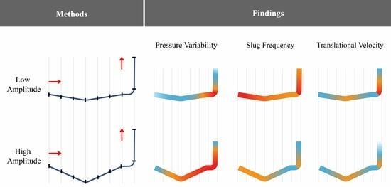
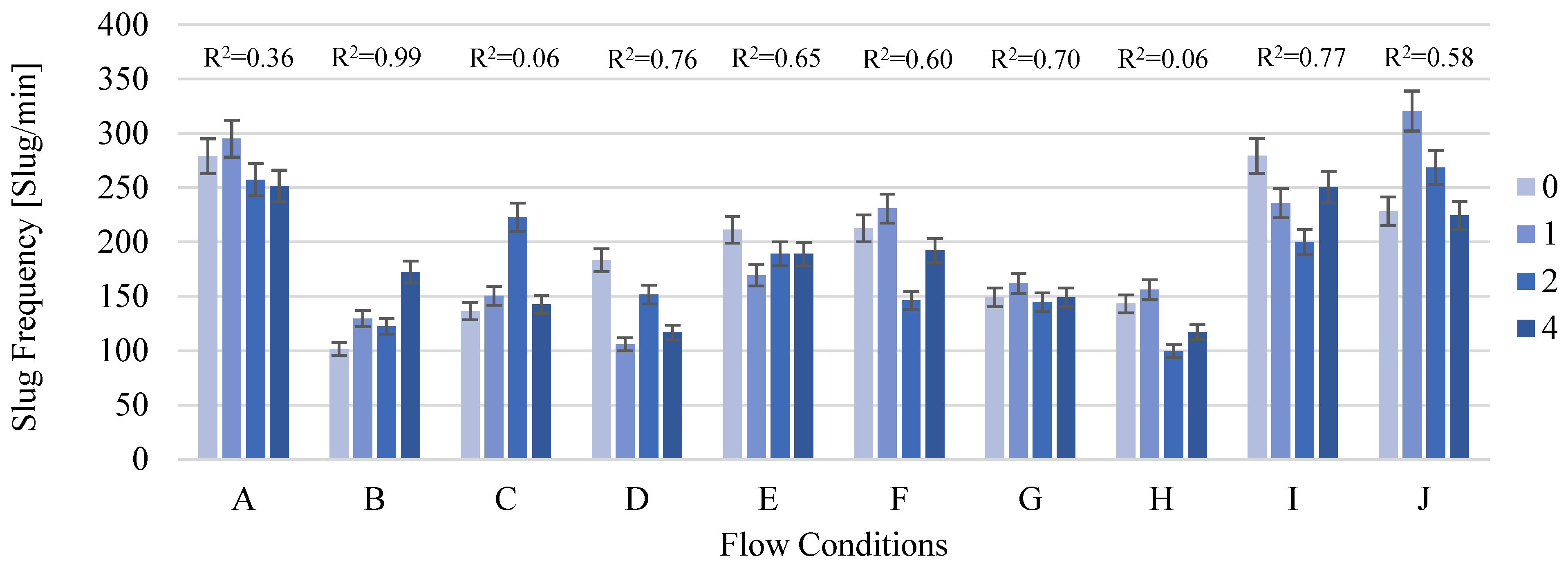
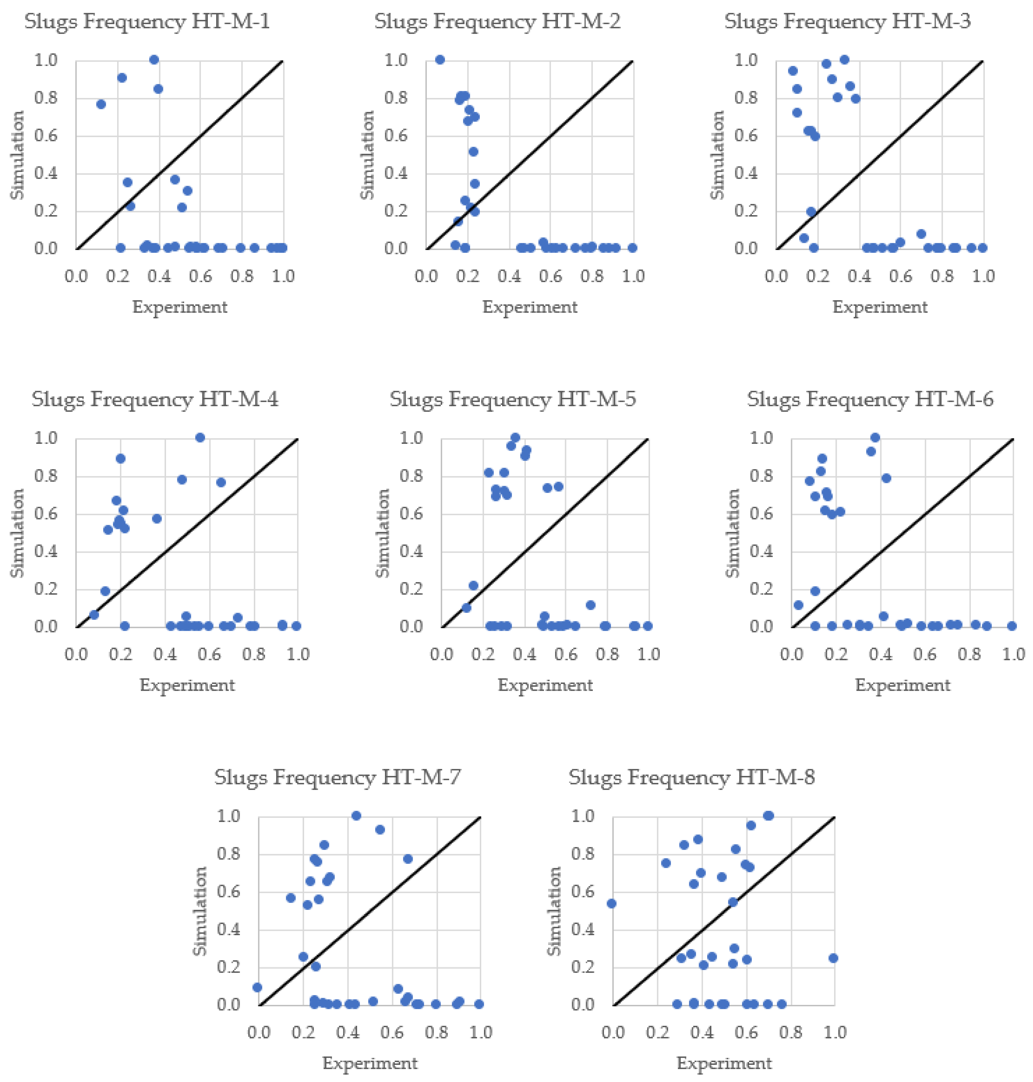
In general, the slug frequency decreases as the undulation amplitude increases, with a few outlier cases.
-
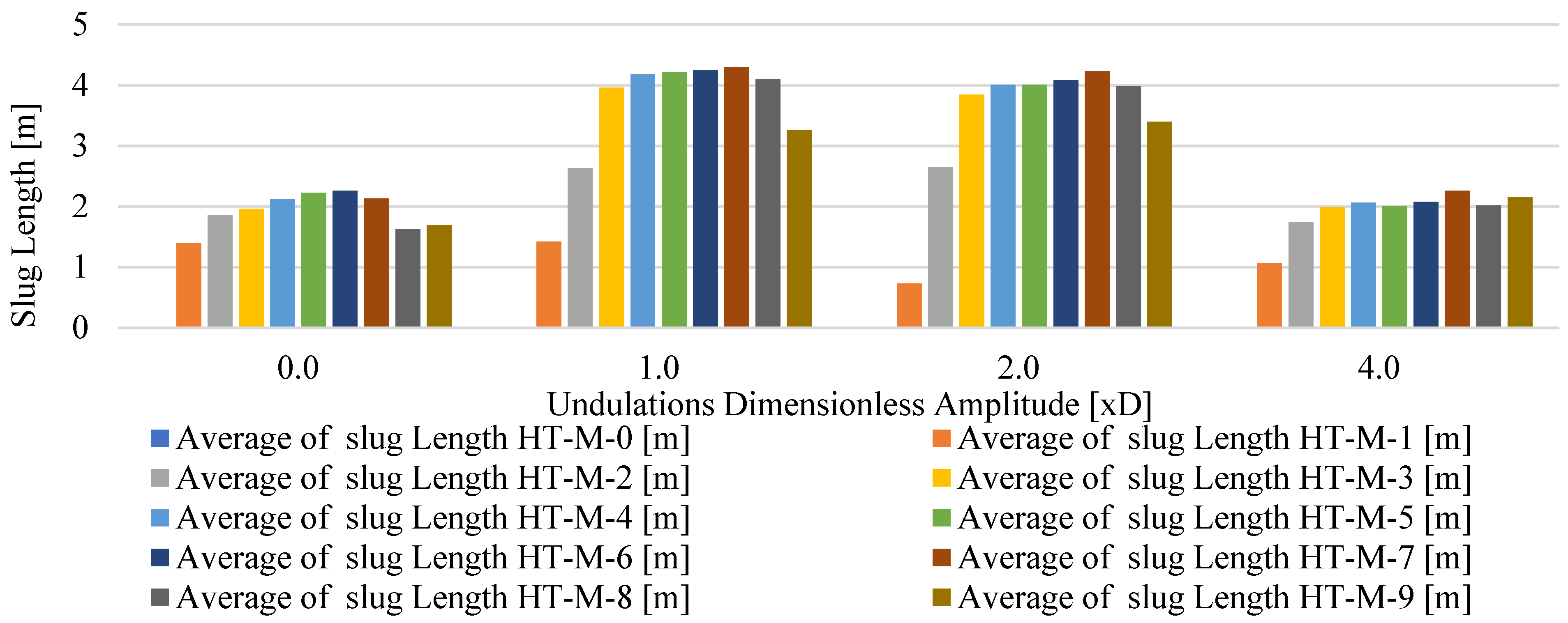
The slug length may either decrease or remain constant with an increasing undulation amplitude, depending on the flow conditions.
-
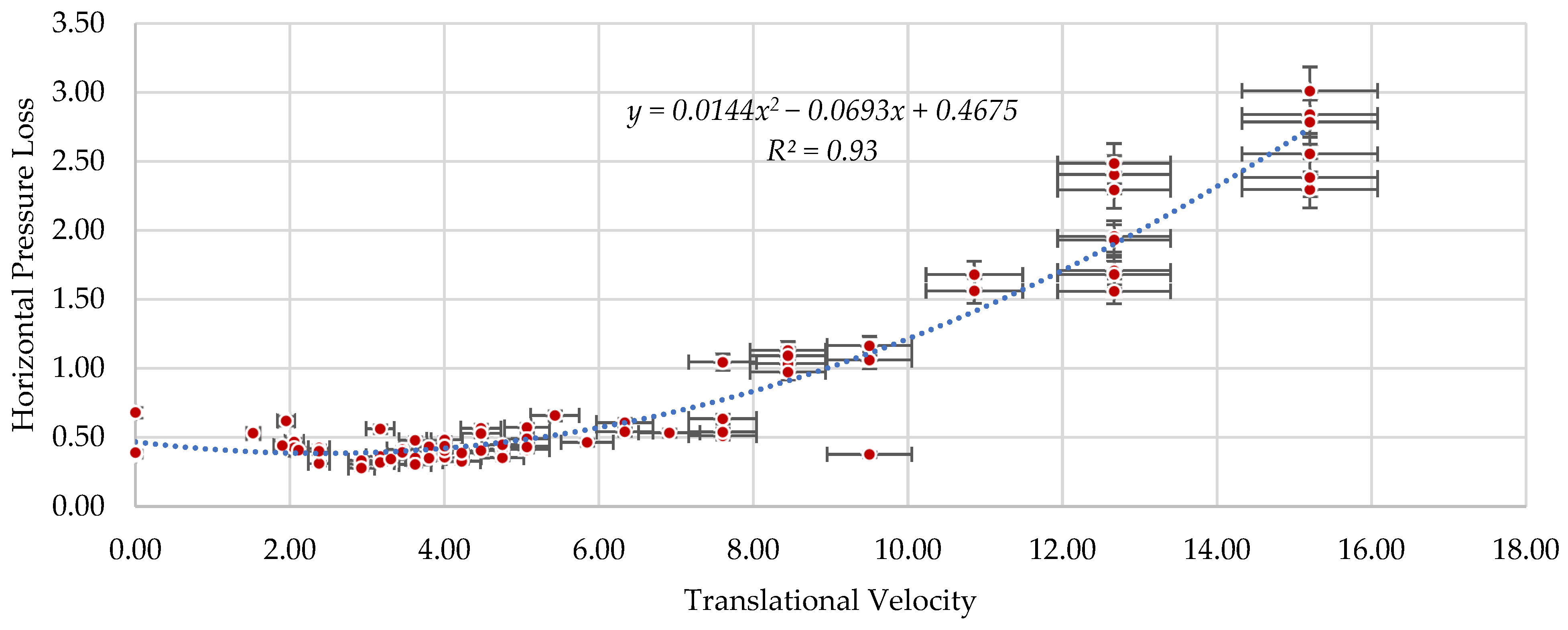
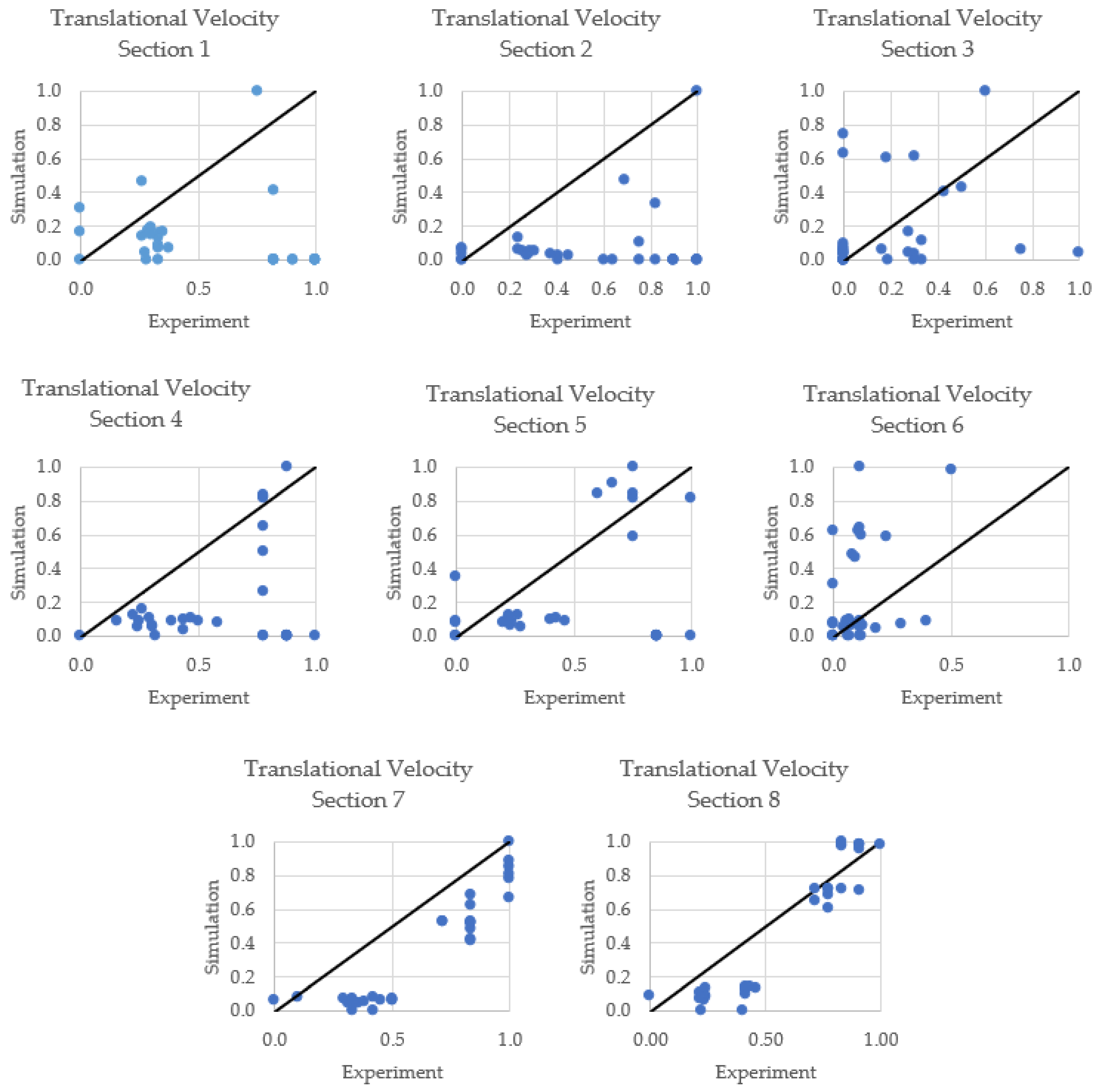
Both higher and lower kinetic energy cases show similar trends except for the translational velocity which is higher for cases of high kinetic energy.
-
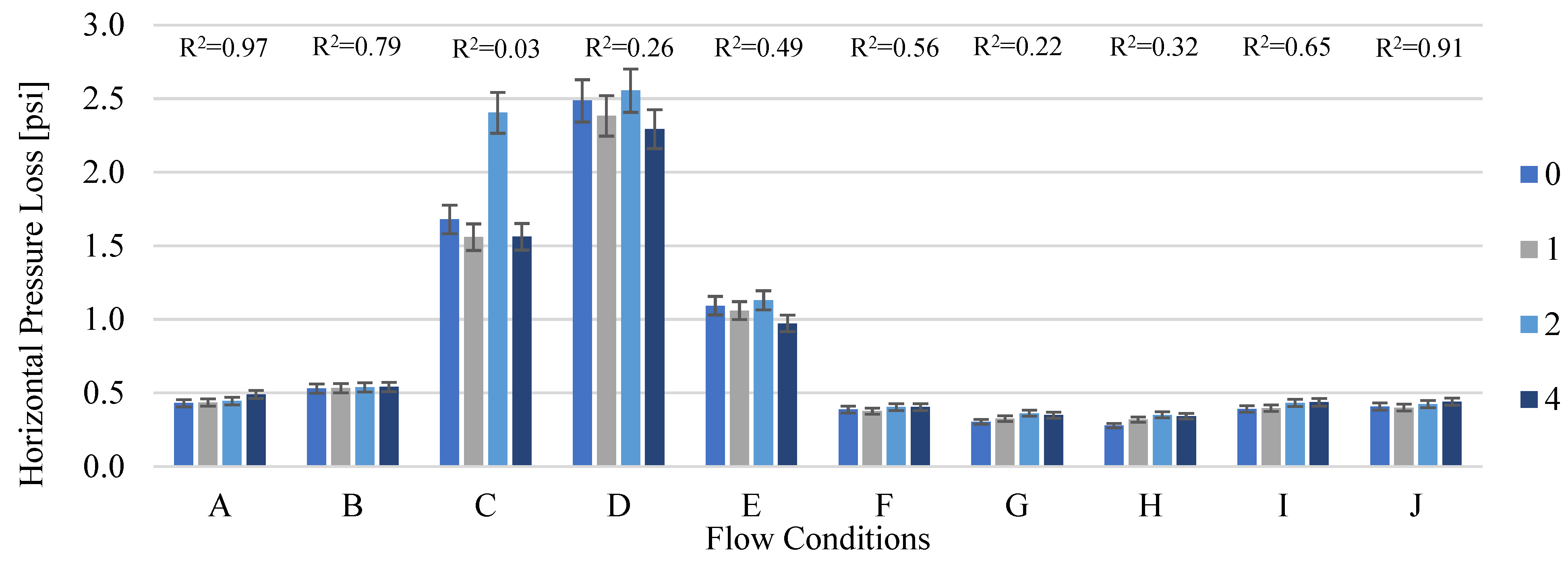
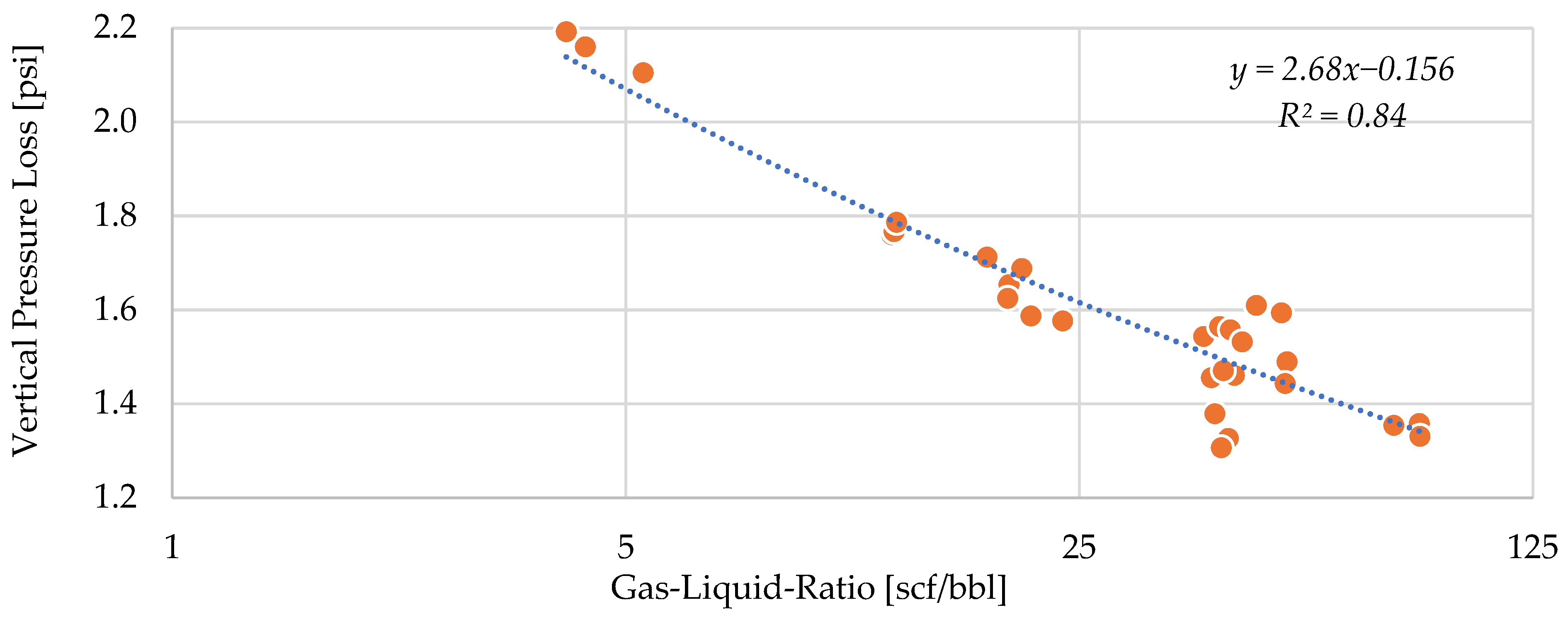
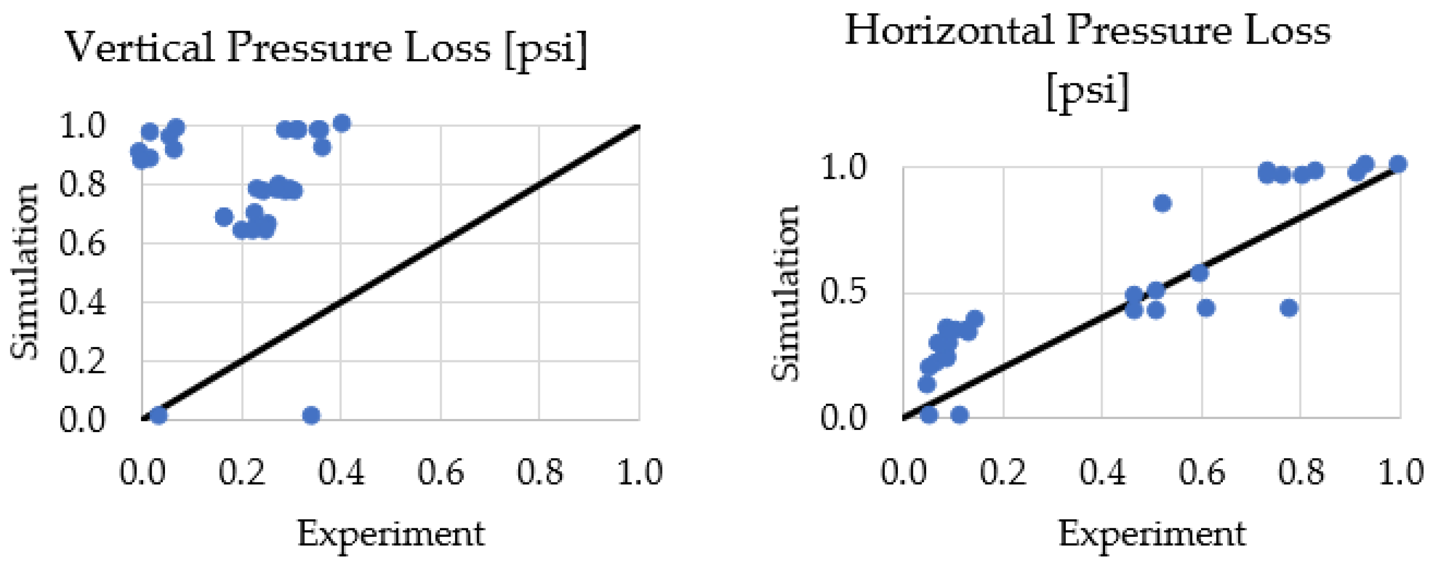
Horizontal and vertical pressure losses increase with higher undulation amplitudes.
-
The variability of pressure at the given location decreases with increased undulation amplitude for cases of high kinetic energy but increases for cases of low energy.
-
Slug merging is observed along the lateral section, resulting in a gradual decrease in slug frequency.
-
The numerical simulation predicts lower translational velocities, higher slug lengths, and lower frequencies compared to the experimental results, with no correlation between the two results (experimental and numerical) explaining the importance of the liquid fallback effect in the studied system’s geometry.
-
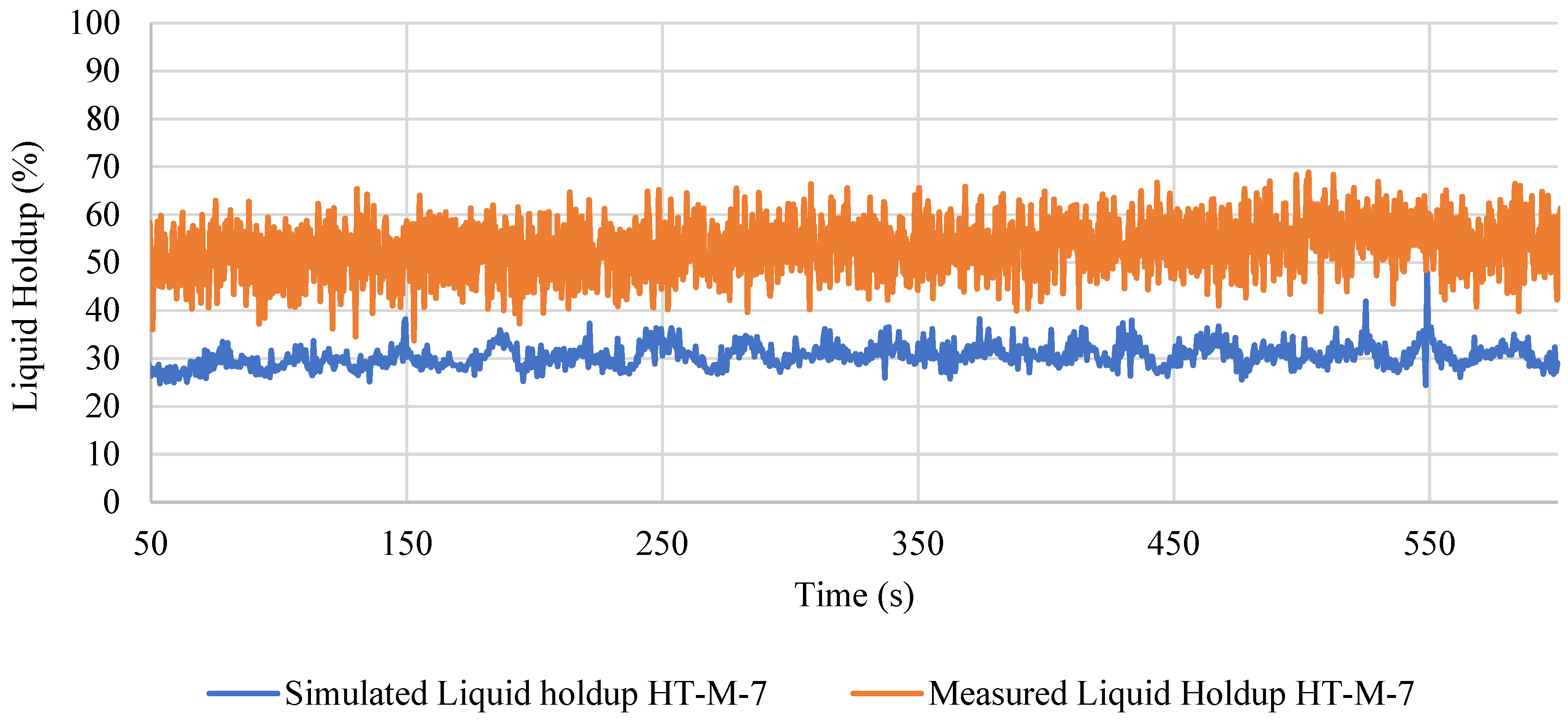
The observed lateral pressure losses are four to five times higher than the numerically obtained pressure losses, likely due to a lack of liquid fallback effect modeling. The lateral section exhibits higher liquid holdup over time in the measured data, as illustrated in Appendix A, Figure A1 and Figure A2.
-
The observed vertical pressure losses agree in magnitude and trend with the numerical simulation results.
The authors recommend further investigation into the effect of undulating frequency (number of undulations) on slug characteristics, pressure losses, and flow stability/variability, with an experimental facility dedicated to liquid fallback quantification.

Supplementary Materials

These are available online at https://data.mendeley.com/datasets/vd2hj27ywy/draft?a=aaec4643-1270-4c5f-95d1-74f581bc170e (accessed on 28 September 2023).

Author Contributions

Y.K.: Conceptualization, Methodology, Investigation, Writing—Original Draft, Data Curation, formal Analysis, Software. K.L.: Validation, Supervision, Writing—Review and Editing. C.T.: Writing—Review and Editing. A.E.A.: Investigation. A.S.F.: Investigation. H.O.: Writing—Review and Editing. All authors have read and agreed to the published version of the manuscript.

Funding

This research was funded by the North Dakota Industrial Commission, grant number 43500-2730.

Data Availability Statement

Generated data are available through KHETIB, Youcef; Ling, Kegang; Feilen, Harry (2023), “University of North Dakota UTP Flow loop Undulations Experiment Data”, Mendeley Data, V3, doi: 10.17632/vd2hj27ywy.3 (See Supplementary Materials).

Acknowledgments

The authors recognize the support of the North Dakota Industrial Commission, Slb for making its OLGA® software available and of Mathworks for making the Matlab® Educational License available. The authors would like to thank Ines Houali for her support regarding graphics editing and the anonymous reviewers for their valuable comments and suggestions, which helped improve the final quality of the paper.

Conflicts of Interest

The authors declare no conflict of interest.

Appendix A

Figure A1 and Figure A2 display history match results of pressure and water holdup parameters for sensor position M-7, situated at the base of the vertical section.
Figure A1. Measured and simulated pressure at PT-M-7 probe location.
Fuels 04 00026 g0a1
Figure A2. Measured and simulated water holdup at HT-M-7 probe location.
Fuels 04 00026 g0a2
Table A1. Calibration results for the probes used in the experimental facility, and the associated measurement uncertainty U95 according to [32].
TagABCMeasurement Uncertainty
HT-M-123.584−17.7422.2765.96
HT-M-2102.720−238.930167.1002.64
HT-M-373.852−169.00092.4103.91
HT-M-442.068−52.8241.8009.43
HT-M-539.419−49.6809.6895.18
HT-M-657.933−108.61049.7534.56
HT-M-712.867−8.0322.7887.90
HT-M-891.940−185.09088.5575.62
HT-M-924.046−29.4873.4046.73
Figure A3. Translational velocity comparison of simulation and experimental values for flow conditions A, B, C, D, E, F, G, H, I, J, and configuration amplitudes of 0, 5, 10, and 20 cm, at each sensor location (HT-M-1, 2, 3, 4, 5, 6, 7, 8).
Fuels 04 00026 g0a3
Figure A4. Slug frequency comparison of simulation and experimental values for flow conditions A, B, C, D, E, F, G, H, I, J, and configuration amplitudes of 0, 5, 10, and 20 cm, at each sensor location (HT-M-1, 2, 3, 4, 5, 6, 7, 8).
Fuels 04 00026 g0a4
Figure A5. Slug length comparison of simulation and experimental values for flow conditions A, B, C, D, E, F, G, H, I, J, and configuration amplitudes of 0, 5, 10, and 20 cm, at each sensor location (HT-M-1, 2, 3, 4, 5, 6, 7, 8).
Fuels 04 00026 g0a5
Figure A6. Pressure loss of simulation and experimental values for flow conditions A, B, C, D, E, F, G, H, I, J, and amplitudes of 0, 5, 10, and 20 cm, for horizontal and vertical sections.
Fuels 04 00026 g0a6
Table A2. Principal components analysis coefficients with regard to the variables.
Principal Component 1Principal Component 2Principal Component 3Principal Component 4
Undulation Amplitude0.00−0.04−0.110.07
Superficial Water Velocity0.180.17−0.060.08
Superficial Air Velocity0.21−0.03−0.04−0.03
Gas to Liquid Ratio0.04−0.360.04−0.19
Translational Velocity VT10.200.060.09−0.10
Translational Velocity VT20.200.060.07−0.11
Translational Velocity VT30.03−0.020.330.33
Translational Velocity VT40.200.020.10−0.04
Translational Velocity VT50.200.070.07−0.08
Translational Velocity VT60.06−0.110.240.40
Translational Velocity VT70.200.010.06−0.08
Translational Velocity VT80.210.030.06−0.05
Slug Length HT-M-10.040.110.30−0.02
Slug Length HT-M-20.010.010.10−0.18
Slug Length HT-M-3−0.050.010.330.22
Slug Length HT-M-40.04−0.170.32−0.12
Slug Length HT-M-50.040.180.11−0.12
Slug Length HT-M-60.00−0.080.260.44
Slug Length HT-M-7−0.050.100.28−0.36
Slug Length HT-M-8−0.130.090.30−0.22
Slug Length HT-M-9−0.130.180.21−0.10
Slug Frequency HT-M-10.170.130.030.18
Slug Frequency HT-M-20.180.140.000.02
Slug Frequency HT-M-30.190.16−0.050.00
Slug Frequency HT-M-40.170.14−0.080.02
Slug Frequency HT-M-50.150.190.02−0.03
Slug Frequency HT-M-60.180.150.06−0.01
Slug Frequency HT-M-70.120.280.09−0.07
Slug Frequency HT-M-8−0.050.110.33−0.06
Slug Frequency HT-M-9−0.090.340.020.06
Variability PT-M-00.050.28−0.140.28
Variability PT-M-10.20−0.130.020.02
Variability PT-M-20.20−0.140.020.02
Variability PT-M-30.20−0.150.000.03
Variability PT-M-40.20−0.150.000.02
Variability PT-M-50.20−0.110.000.03
Variability PT-M-60.21−0.09−0.020.00
Variability PT-M-70.21−0.08−0.03−0.02
Variability PT-M-80.21−0.070.00−0.03
Variability PT-M-90.210.01−0.04−0.04
Horizontal Pressure Loss0.200.08−0.03−0.07
Vertical Pressure Loss−0.040.38−0.170.07

References

  1. Khetib, Y.; Ling, K.; Allam, L.; Aoun, A.E. Statistical and Numerical Investigation of the Effect of Wellbore Trajectories in Williston Basin Horizontal Wells and Their Effects on Production Performance. Pet. Petrochem. Eng. J. 2022, 6, 320–335. [Google Scholar] [CrossRef]
  2. Norris, H.L.; Lee, H. The Use of a Transient Multiphase Simulator to Predict and Suppress Flow Instabilities in a Horizontal Shale Oil Well. SPE 2012, 1009–1019. [Google Scholar] [CrossRef]
  3. Khetib, Y.; Rasouli, V.; Rabiei, M.; Chellal, H.A.K.; Abes, A.; Bakelli, O.; Aoun, A.E. Modelling Slugging Induced Flow Instabilities and Its Effect on Hydraulic Fractures Integrity in Long Horizontal Wells. In Proceedings of the 56th U.S. Rock Mechanics/Geomechanics Symposium, American Rock Mechanics Association, Santa Fe, NJ, USA, 26–29 June 2022; pp. 1–8. [Google Scholar] [CrossRef]
  4. Lu, H.; Anifowosh, O.; Xu, L. Understanding the Impact of Production Slugging Behavior on Near-Wellbore Hydraulic Fracture and Formation Integrity. In Proceedings of the SPE International Symposium on Formation Damage Control, OnePetro, Lafayette, LA, USA, 23–24 February 2018; pp. 7–9. [Google Scholar] [CrossRef]
  5. Khetib, Y. Investigation of Transient Multiphase Flow Performance in Undulating Horizontal Unconventional Wells; University of North Dakota: Grand Forks, ND, USA, 2022. [Google Scholar]
  6. Khetib, Y.; Aoun, A.E.; Ling, K. Experimental and Numerical Analysis of Toe-Up Trajectory Inclination Angle and Gas Lift Rate Effect on Unconventional Oil Well Performance. In Proceedings of the SPE/AAPG/SEG Unconventional Resources Technology Conference, OnePetro, Denver, CO, USA, 13–15 June 2023; pp. 1–21. [Google Scholar] [CrossRef]
  7. Zhang, H.; Falcone, G.; Valko, P.P.; Teodoriu, C. Numerical Modeling of Fully-Transient Flow in the Near-Wellbore Region During Liquid Loading in Gas Wells. In Proceedings of the Latin American and Caribbean Petroleum Engineering Conference, Port of Spain, Trinidad and Tobago, 14–15 June 2023; pp. 1–15. [Google Scholar] [CrossRef]
  8. Tang, H.; Hasan, A.R.; Killough, J.; Hasan, A.R.; Killough, J. Development and Application of a Fully Implicitly Coupled Wellbore/Reservoir Simulator To Characterize the Transient Liquid Loading in Horizontal Gas Wells. SPE J. 2018, 23, 1615–1629. [Google Scholar] [CrossRef]
  9. Veeken, K.; Hu, B.; Schiferli, W. Gas-Well Liquid-Loading-Field-Data Analysis and Multiphase-Flow Modeling. SPE Prod. Oper. 2010, 25, 275–284. [Google Scholar] [CrossRef]
  10. Kannan, S.; Nagoo, A.; Lea, J. Understanding Heel Dominant Liquid Loading in Unconventional Horizontal Wells. In Proceedings of the SPE Annual Technical Conference and Exhibition, OnePetro, Calgary, AB, Canada, 30 September–2 October 2019; pp. 1–13. [Google Scholar] [CrossRef]
  11. Tang, H.; Chai, Z.; He, Y.; Xu, B.; Hasan, A.R.; Killough, J. What Happens after the Onset of Liquid Loading?—An Insight from Coupled Well-Reservoir Simulation. In Proceedings of the SPE Annual Technical Conference and Exhibition, Dallas, TX, USA, 24–26 September 2018; pp. 24–26. [Google Scholar] [CrossRef]
  12. Jackson, D.F.B.; Virueś, C.J.J.; Sask, D. Investigation of Liquid Loading in Tight Gas Horizontal Wells with a Transient Multiphase Flow Simulator. In Proceedings of the Society of Petroleum Engineers—Canadian Unconventional Resources Conference 2011, CURC 2011, Calgary, AB, Canada, 15–17 November 2011; Volume 3, pp. 2256–2265. [Google Scholar] [CrossRef]
  13. Adaze, E.; Al-Sarkhi, A.; Badr, H.M.; Elsaadawy, E. Current status of CFD modeling of liquid loading phenomena in gas wells: A literature review. J. Pet. Explor. Prod. Technol. 2019, 9, 1397–1411. [Google Scholar] [CrossRef]
  14. Tang, H.; Hasan, A.R.; Killough, J. A Fully-Coupled Wellbore-Reservoir Model for Transient Liquid Loading in Horizontal Gas Wells. In Proceedings of the SPE Annual Technical Conference and Exhibition, San Antonio, TX, USA, 9–11 October 2017; pp. 1–19. [Google Scholar] [CrossRef]
  15. Khetib, Y.; Zunez, S. Integrated Pipeline and Wells Transient Behavior of CO2 Injection Operations: Flow Assurance Best Practices. In Proceedings of the PSIG Annual Meeting, OnePetro, San Antonio, TX, USA, 19 May 2023; pp. 1–25. Available online: https://onepetro.org/PSIGAM/proceedings/PSIG23/All-PSIG23/PSIG-2325/520097 (accessed on 22 July 2023).
  16. Khan, S.; Khulief, Y.A.; Al-Shuhail, A.A. The effect of injection well arrangement on CO2 injection into carbonate petroleum reservoir. Int. J. Glob. Warm. 2018, 14, 462–487. [Google Scholar] [CrossRef]
  17. Pekot, L.J.; Petit, P.; Adushita, Y.; Saunier, S.; De Silva, R. Simulation of Two-Phase Flow in Carbon Dioxide Injection Wells. In Proceedings of the Society of Petroleum Engineers—Offshore Europe Oil and Gas Conference and Exhibition 2011, OE 2011, Aberdeen, UK, 6–8 September 2011; Volume 1, pp. 94–106. [Google Scholar] [CrossRef]
  18. Loizzo, M.; Lecampion, B.; Bérard, T.; Harichandran, A.; Jammes, L. Reusing O&G Depleted Reservoirs for CO2 Storage: Pros and Cons. In Proceedings of the Society of Petroleum Engineers—Offshore Europe Oil and Gas Conference and Exhibition 2009, OE 2009, Aberdeen, UK, 8–11 September 2009; Volume 2, pp. 783–792. [Google Scholar] [CrossRef]
  19. Haigh, M.J. Well Design Differentiators for CO2 Sequestration in Depleted Reservoirs. In Proceedings of the Society of Petroleum Engineers—Offshore Europe Oil and Gas Conference and Exhibition 2009, OE 2009, Aberdeen, UK, 8–11 September 2009; Volume 2, pp. 719–731. [Google Scholar] [CrossRef]
  20. Cronshaw, M.B.; Bolling, J.D. A Numerical Model of the Non-Isothermal Flow of Carbon Dioxide in Wellbores. In Proceedings of the Society of Petroleum Engineers—SPE California Regional Meeting, CRM 1982, San Francisco, CA, USA, 24–26 March 1982; pp. 173–180. [Google Scholar] [CrossRef]
  21. Paterson, L.; Lu, M.; Connell, L.D.; Ennis-King, J. Numerical Modeling of Pressure and Temperature Profiles Including Phase Transitions in Carbon Dioxide Wells. In Proceedings of the SPE Annual Technical Conference and Exhibition 2008, Denver, CO, USA, 21–24 September 2008; Volume 4, pp. 2693–2703. [Google Scholar] [CrossRef]
  22. Tran, N.; Karami, H. Transient Multiphase Analysis of Well Trajectory Effects in Production of Horizontal Unconventional Wells. In Proceedings of the SPE Oklahoma City Oil and Gas Symposium, OnePetro, Oklahoma City, OK, USA, 9 April 2019; pp. 1–13. [Google Scholar] [CrossRef]
  23. Nair, J.; Pereyra, E.; Sarica, C. Existence and Prediction of Severe Slugging in Toe-Down Horizontal Wells. In Proceedings of the SPE Annual Technical Conference and Exhibition, OnePetro, Dallas, TX, USA, 24–26 September 2018; pp. 1–19. [Google Scholar] [CrossRef]
  24. Pankaj, P.; Patron, K.E.; Lu, H. Artificial Lift Selection and Its Applications for Deep Horizontal Wells in Unconventional Reservoirs. URTeC Tech. 2018, 23–25. [Google Scholar] [CrossRef]
  25. Dinata, R.; Sarica, C.; Pereyra, E. End of Tubing EOT Placement Effects on the Two-Phase Flow Behavior in Horizontal Wells: Experimental Study. In Proceedings of the SPE Annual Technical Conference and Exhibition, Indianapolis, IN, USA, 23–25 May 2016; pp. 26–28. [Google Scholar] [CrossRef]
  26. Brito, R.M. Effect of Horizontal Well Trajectory on Two-Phase Gas-Liquid Flow Behavior. Ph.D. Dissertation, The University of Tulsa, Tulsa, OK, USA, 2015. [Google Scholar]
  27. Brito, R.; Pereyra, E.; Sarica, C. Existence of Severe Slugging in Toe-Up Horizontal Gas Wells. In Proceedings of the Society of Petroleum Engineers—SPE North America Artificial Lift Conference and Exhibition 2016, The Woodlands, TX, USA, 25–27 October 2016; pp. 25–27. [Google Scholar] [CrossRef]
  28. Brito, R.; Pereyra, E.; Sarica, C. Well trajectory effect on slug flow development. J. Pet. Sci. Eng. 2016, 167, 366–374. Available online: http://onepetro.org/BHRNACMT/proceedings-pdf/BHR16/All-BHR16/BHR-2016-053/1330257/bhr-2016-053.pdf (accessed on 24 June 2021). [CrossRef]
  29. Tran, N.L.; Orazov, B.; Karami, H. Impacts of Well Geometry and Gas Lift on Flow Dynamic and Production of Unconventional Horizontal Wells. In Proceedings of the SPE Artificial Lift Conference and Exhibition—Americas, Galveston, OnePetro, Galveston, TX, USA, 23–25 August 2022; pp. 1–16. [Google Scholar] [CrossRef]
  30. Gokcal, B. An Experimental and Theoretical Investigation of Slug Flow for High Oil Viscosity in Horizontal Pipes. Ph.D. Dissertation, University of Tulsa, Tulsa, OK, USA, 2008. [Google Scholar]
  31. OLGA 2020.2. User Manual. 2020. Available online: https://www.software.slb.com/products/olga (accessed on 15 August 2023).
  32. Dieck, R.H. Measurement uncertainty models. ISA Trans. 1997, 36, 29–35. [Google Scholar] [CrossRef]
Figure 1. Schematic diagram of the UTP flow-loop facility at the University of North Dakota, from [5].
Fuels 04 00026 g001
Figure 2. Illustration of undulation amplitude and inclination angle in the experimental system, from [6].
Fuels 04 00026 g002
Figure 3. Photo of the flow-loop facility and assigned computer and DAQ station, from [6].
Fuels 04 00026 g003
Figure 4. Municipal water and test liquid rheogram data, from [5].
Fuels 04 00026 g004
Figure 5. Figures (ad) illustrate the cases with one undulation and amplitudes of 0 cm, 5 cm, 10 cm, and 20 cm, respectively.
Fuels 04 00026 g005
Figure 6. Slug translational velocity versus undulation amplitude for flow conditions A to J in a single undulation case.
Fuels 04 00026 g006
Figure 7. Slug frequency versus undulation amplitude for flow conditions A to J in a single undulation case.
Fuels 04 00026 g007
Figure 8. Slug length versus undulation amplitude for flow conditions from A to J in a single undulation case.
Fuels 04 00026 g008
Figure 9. Averaged horizontal pressure loss versus as a function of the undulation’s amplitude for flow conditions from A to J in a single undulation case.
Fuels 04 00026 g009
Figure 10. Horizontal pressure loss versus HT-M-7 translational velocity correlation, for A, B, C, D flow conditions.
Fuels 04 00026 g010
Figure 11. Vertical pressure loss versus undulation amplitude for flow conditions from A to J in a single undulation case.
Fuels 04 00026 g011
Figure 12. Lateral pressure variability as a function of undulation amplitude for flow conditions from A to J.
Fuels 04 00026 g012
Figure 13. Slug frequency for each water holdup probe of the lateral section plotted against the dimensionless undulation amplitude.
Fuels 04 00026 g013
Figure 14. Slug length for each water holdup probe of the lateral section plotted against the undulation’s dimensionless amplitude.
Fuels 04 00026 g014
Figure 15. Slug translational velocity for each water holdup probe of the lateral section versus dimensionless undulation amplitude.
Fuels 04 00026 g015
Figure 16. Pressure variability profile plotted against the undulation’s dimensionless amplitude.
Fuels 04 00026 g016
Figure 17. Principal components analysis results for PC1 and PC2.
Fuels 04 00026 g017
Figure 18. Vertical pressure loss versus gas–liquid ratio with trend line equation and R2.
Fuels 04 00026 g018
Figure 19. Simulation translational velocity profile versus undulation amplitude.
Fuels 04 00026 g019
Figure 20. Simulation slug frequency profile versus undulation’s dimensionless amplitude.
Fuels 04 00026 g020
Figure 21. Simulation slug length profile along the lateral and vertical sections plotted against the undulation’s dimensionless amplitude.
Fuels 04 00026 g021
Figure 22. Simulation lateral time-averaged pressure loss plotted against the flow conditions A to J, see Table 3, for different undulation dimensionless amplitudes.
Fuels 04 00026 g022
Figure 23. Simulation lateral time-averaged pressure loss versus plotted against the flow conditions A to J, see Table 3, for different undulation dimensionless amplitudes.
Fuels 04 00026 g023
Table 1. Flow-loop facility characteristics.
Equipment NameTagModel NameSpecifications
Air CompressorCMP-G-1Ingersoll Rand
Model 7100
15 hp, max pressure 175 psig, 50 CFM
Water PumpPMP-W-1Gorman-Rupp
Model 3790-95
7.5 hp, max pressure 75 psig, max flowrate 157 gpm
Liquid TankTNK-W-1Schutz275 gallons
High-Speed CameraCAM-N-1Z-CAM E260 fps, max resolution
Pressure RegulatorPR-G-1Ingersoll RandRange (0 to 160 psig)
Heat ExchangerEX-G-1Ingersoll RandFlowrate 64 cfm max temperature 140 F, max pressure 203 psig
Table 2. Experimental cases, undulation amplitude, and number configuration.
CaseCodeNumber of UndulationsPositionAmplitude (cm)
±0.1 cm
Angle (°)
±1°
11U20A1−202015.26
21U10A1−10107.56
31U5A1−553.77
40U0A0000.00
Table 3. Flow conditions and corresponding mass and volumetric flow rates and superficial velocities for water mixture and air in the experiment.
ParameterFlow Conditions
ABCDEFGHIJUnit
Water Flow Rate10.0 110.0 120.0 128.0 120.0 15.0 12.5 12.5 110.0 110.0 1GPM
Water Superficial Velocity1.00 11.02 12.04 12.86 12.04 10.51 10.26 10.26 11.02 11.02 1ft/s
Mass Flow Rate0.6 10.63 11.26 11.77 11.26 10.32 10.16 10.16 10.63 10.63 1Kg/s
Air Flow Rate5.0 210.0 320.0 333.0 310.0 35.0 25.0 22.8 22.8 21.1 2SCFM
Air Superficial Velocity3.82 27.64 315.28 325.21 37.63 33.83 23.83 22.15 22.15 20.80 2ft/s
Mass Flow Rate0.003 20.006 30.012 30.020 30.006 30.003 20.003 20.0017 20.002 20.0006 2Kg/s
1 Measurement Uncertainty: ±1.0%. 2 Measurement Uncertainty: ±3%. 3 Measurement Uncertainty: ±1.5%.
Disclaimer/Publisher’s Note: The statements, opinions and data contained in all publications are solely those of the individual author(s) and contributor(s) and not of MDPI and/or the editor(s). MDPI and/or the editor(s) disclaim responsibility for any injury to people or property resulting from any ideas, methods, instructions or products referred to in the content.

