Article

Stress-Dependent Petrophysical Properties of the Bakken Unconventional Petroleum System: Insights from Elastic Wave Velocities and Permeability Measurements

College of Engineering and Mines, University of North Dakota, Grand Forks, ND 58202, USA
*
Author to whom correspondence should be addressed.
Fuels 2023, 4(4), 397-416; https://doi.org/10.3390/fuels4040025
Submission received: 10 August 2023 / Revised: 4 September 2023 / Accepted: 22 September 2023 / Published: 30 September 2023

Abstract

:
The net-effective stress is a fundamental physical property that undergoes dynamic changes in response to variations in pore pressure during production and injection activities. Petrophysical properties, including porosity, permeability, and wave velocities, play a critical role and exhibit strong dependence on the mechanical stress state of the formation. The Williston basin’s Bakken Formation represents a significant reservoir of hydrocarbons within the United States. To investigate this formation, we extracted core plugs from three distinct Bakken members, namely Upper Bakken, Middle Bakken, and Lower Bakken. Subsequently, we conducted a series of measurements of ultrasonic compressional and shear wave velocities, as well as pulse decay permeabilities using nitrogen, under various confining pressures employing the Autolab-1500 apparatus. Our experimental observations revealed that the ultrasonic wave velocities and permeability display a significant sensitivity to stress changes. We investigated existing empirical relationships on velocity-effective stress, compressional-shear wave velocities, and permeability-effective stress, and proposed the best models and associated fitting parameters applicable to the current datasets. In conjunction with the acquired datasets, these models have considerable potential for use in time-lapse seismic monitoring and the study of production decline behavior. The best fitting models can be used to forecast the petrophysical and geomechanical property changes as the reservoir pore pressure is depleted due to the production, which is critical to the production forecast for unconventional reservoirs.

1. Introduction

The Bakken formation, situated in North Dakota, Montana, and sections of Canada, have emerged as significant contributors to North American oil production as a result of their extensive resources and innovative extraction techniques [1]. Nevertheless, the geological complexity of the Bakken Formation contributes to both its richness and its hydrocarbon recovery difficulties. It consists of three layers: upper and lower shale strata that act as source rocks and a sandstone/siltstone formation that acts as a reservoir [2]. The highly heterogeneous nature of this unconventional reservoir necessitates the use of cutting-edge technologies, including hydraulic fracturing and horizontal drilling [3]. This geological complexity requires cautious management to maximize resource extraction, which requires efficient production and/or injection design and monitoring during hydrocarbon production.
During production or injection, subsurface external stresses and pore pressures change. Reservoir rock properties, including elastic properties and flow properties, are sensitive to these variations in stress. Stress affects permeability, one of the critical parameters that regulate flow. Experimental studies conducted in the past [4,5] provide evidence of permeability’s dependence on stress. Later on, researchers discovered that stress-dependent permeability plays important role in a variety of engineering applications, including hydrocarbon production and fluid injection designs [6,7], CO2 sequestration [8], coal bed methane reservoirs [9,10], geothermal reservoirs [11], and nuclear waste storage in the subsurface.
Stress-dependent permeability studies are broadly classified into three groups: experimental, development of empirical and analytical models, and the numerical simulation studied. Experimental studies provided the initial evidence of stress-dependent permeability [4], and further studies tried to understand the effect of fluid pressure and external confining pressure independently on stress-dependent permeability and proposed effective stress laws [5]. Furthermore, the stress-dependent permeability behavior of reservoir rocks in laboratory conditions was investigated on various rock types [12,13,14,15,16]. These studies emphasize that stress-dependent permeability is crucial in production design and history matching for reservoir management, wellbore stability, and accurate forecasting. It influences reservoir behavior, production rates, and pressure profiles, ensuring efficient hydrocarbon recovery [17,18]. Experimental studies carried out on the core scale can be utilized to build empirical models that can be used at the field scale with appropriate calibrations [18].
In the realm of reservoir monitoring and exploration, the velocity of elastic waves traveling through a medium holds paramount significance [19]. This elastic wave velocity is influenced by multiple factors, including density, rigidity, and the in situ stress conditions within the medium, among others [20]. Consequently, when stress variations occur within a reservoir due to activities such as hydrocarbon extraction, or the injection of fluids for enhanced oil recovery or carbon capture and geological storage, it imparts alterations to the mechanical properties of the reservoir rocks and, as a result, modifies the velocity of seismic waves propagating through the subsurface [21]. To comprehend and quantify these changes in elastic wave velocities, time-lapse seismic surveys, commonly known as “4D” seismic surveys, are employed [19]. The variations in elastic wave velocities, observed through such surveys, furnish valuable insights into the dynamic stress conditions prevailing within the reservoir and helps in the effective management of the extraction or injection processes, estimating the remaining reserves, and evaluating the overall integrity of the reservoir. Again, core scale ultrasonic wave velocity measurements in the laboratory provide crucial inputs to model the stress-sensitive elastic wave velocities.
The significance of selecting suitable models cannot be overstated in the realms of efficient production/injection design and dynamic reservoir monitoring. In this paper, we conducted a comprehensive review of existing empirical models concerning the elastic wave velocities evolution with stress, the permeability evolution with stress, and the relationships between longitudinal and transverse wave velocities for the Bakken unconventional petroleum system. By thoroughly examining these models, we aimed to provide researchers and reservoir engineers with valuable insights to facilitate their selection of appropriate models and fitting parameters when addressing Bakken reservoirs in practical applications. These models serve as valuable tools to enhance our understanding of the complex interactions within the Bakken reservoirs, aiding in the optimization of production and injection strategies and supporting effective dynamic reservoir monitoring practices.
This paper’s structure is as follows: In 
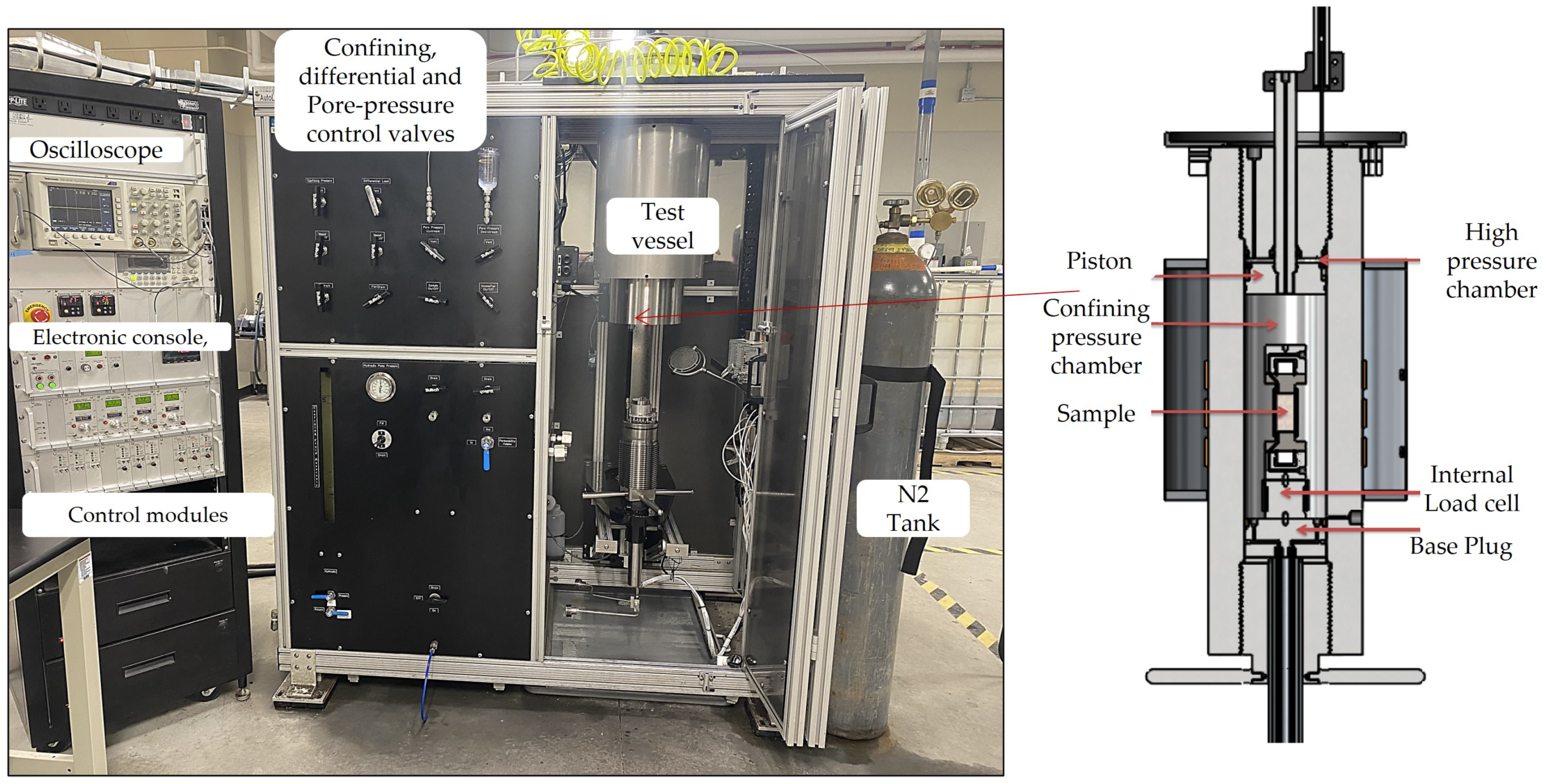
Section 2, we explain the experimental procedures, review existing empirical models, and providd a concise overview of the Bakken petroleum system. In Section 3, we present the outcomes obtained through the application of various empirical models. Finally, the Section 4 offers interpretations of the results, comparisons between different models, proposals for the most suitable models, comparisons with previous research, and a presentation of identified limitations, as well as suggestions for future research directions.

2. Materials and Methods

In this section, we first described the experimental procedures and then reviewed the widely used empirical equations of velocity-effective stress, permeability-effective stress, as well as compressional-shear wave velocities. Afterward, we provided an explanation of the geological and petrophysical characteristics specific to the Bakken petroleum system.

2.1. Experimental Procedures

The AutoLab-1500 facility, supplied by New England Research, Inc. (White River Junction, VT, USA), was utilized for conducting elastic and mechanical experiments in the current research (Figure 1). Testing can be carried out under various scenarios of confining pressures, pore pressure, and temperature. The system enables the execution of conventional rock mechanics testing protocols, including isotropic compression, uniaxial compression, triaxial compression, viscoelastic deformation, elastic waveform measurements, and steady-state and transient permeability measurements, etc., [22,23]. The system has the capability to operate within two different pressure ranges of up to 10,000 or 20,000 psi, along with temperatures up to 248 F [22]. All the experiments in the present study are carried out at drained condition.

2.1.1. Ultrasonic Wave Velocity Experiments

In the sonic wave experiment, the transmission of compressional wave (P-wave), two perpendicular shear waves (S-wave) through core plugs were recorded. The following procedure was followed:
  • A 1 inch diameter cylindrical-shaped core plug was prepared.
  • The dimensions, density, porosity, and volume of the core plugs were measured.
  • The sample was covered with copper foil and inserted into a pliable jacket. Then, the jacket was sealed to the end plugs with a section of rubber tubing. The rubber jacket was secured to the end plugs at two points with several wraps of steel wire.
  • The ultrasonic end-caps had a native frequency 750 MHz. They included a piezoelectric crystal stack with a p wave and 2 orthogonally polarized shear waves.
  • The sample was secured to the source ultrasonic transducer velocity assembly (PS1) after applying a shear wave couplant to the face of the transducers using a section of elastomer jacket with the same inside diameter as the test specimen. The rubber jacket was attached to the transducer assembly at two points with several warps of steel wire. The other transducer was secured to the specimen with a section of rubber tubing as described above.
  • We connected the receiver ultrasonic transducer velocity assembly (PS2) ultrasonic velocity transducer output to the core plug; we made sure that the connections were in the correct position.
  • We placed the transducer assembly, together with the jacketed specimen, into the pressure vessel.
  • We set the servo-controllers to panel mode and then turned the control knobs fully counterclockwise.
  • We turned on the hydraulic power supply and filled the pressure chamber with mineral oil, which is used to apply confining pressure.
  • We advanced the axial piston inside the vessel approximately 5 mm and closed the valve between the intensifier and the vessel.
  • We adjusted confinement pressure to the required level and started the AutoLab Software to initiate the data acquisition
  • In the control panel, we selected the PS2 ultrasonic velocity transducer under the transducer selection. Then, we set the gain and attenuation information for the pulse-receiver.
  • We verified the waveforms for primary and secondary wave velocities. We located the oscilloscope panel and configured the scope to obtain a clear waveform for a P-wave. Upon obtaining satisfactory waveforms for the primary wave, we verified the S1 and S2 waveforms to ensure that there was sufficient amplitude near the initial onset of the shear wave for precise velocity measurements.
  • We set the sampling interval and recorded the data. We set the desired confining pressure values and at each confining pressure collected the data.

2.1.2. Permeability Measurements

Due to the fact that the permeability of tight rock is very low, the steady-state method is not appropriate in this case. In this study, Bakken core permeability is measured by one of the unsteady-state methods, the pressure pulse method. The following steps were used to run the experiment to determine permeability:
  • The core plug was covered with copper foil and inserted into a pliable jacket. Then, the jacket was sealed to the end plugs with a section of rubber tubing. The rubber jacket was secured to the end plugs at two points with several wraps of steel wire. During the experiment, the end plugs were used to obtain uniform flow of testing fluid to the upstream inlet and out the downstream outlet of the sample.
  • The sample was then transferred into the chamber and affixed with a core holder.
  • Mineral oil was introduced into the vessel in order to generate confining pressure. The confining pressure was raised to the appropriate magnitude.
  • The upstream chamber was filled with dry nitrogen (N2), and the pressure in the reservoir was then raised to the predefined value. The reservoir located downstream was maintained at ambient pressure. It should be noted that the confining stress had to exceed the pressure of the upstream chamber.
  • A connection was made between the upstream chamber and the core plug by opening the valve. The commencement time was documented at that moment. Throughout the duration of the test, data were properly documented. The confining pressures were maintained at a constant level. Upstream and downstream pressures were collected and tracked throughout the sampling process.
  • The pore pressure at the upstream endpoint was monitored and kept constant and the pore pressure at the downstream outlet gradually increased as the N2 flowed through the core sample.
  • We kept the gas flowing until the pressure in the upstream and downstream chambers reached equilibrium within a given tolerance level.
  • We generated pressure pulses at the upstream, waited for the pressure pulses to travel through the core sample and arrive at the downstream reservoir. We waited for the pressure pulses to dissipate and finish the pressure pulse test.
  • The pore pressure in the upstream and downstream chambers was released, resulting in a depletion of both upstream and downstream pressures.
  • We released mineral oil to deplete confining stress.
  • We retrieved the core sample from AutoLab 1500 core holder and finished the experiment.
  • We calculated permeability using the recorded data.

2.2. Velocity-Effective Stress Relationships

In recent decades, extensive research has focused on studying the impact of confining stress on elastic wave velocities. In our investigation, we have curated a selection of four prominent empirical models that have demonstrated widespread success among researchers [24,25]. It is relevant to acknowledge that these models do not constitute an exhaustive compilation of all available options.
Hardin and Richart Jr. (1963) [26] conducted laboratory experiments to assess the elastic wave velocities in samples of Ottawa rocks, crushed quartz, and silt. The wave velocities of these sands showed a relationship with the confining pressure that followed an approximately 1/4 power law. Later, Kopperman et al. (1982) [27] conducted. Wave velocity measurement experiments under isotropic, biaxial, and triaxial loading to investigate the correlation between ultrasonic wave velocities and the stress state in dry rocks. Subsequently, a straightforward power–law model was proposed to describe the relationship between effective stress and velocity.
V p = V p i σ e a
where V p (m/s) is the compressional velocity, σ e (MPa) is the effective isotropic confining stress, V p i (m/s) is the initial compressional velocity at the initial stress state, and a is the fitting parameter. In these experiments, the samples were dry and there was no pore pressure. Therefore, the effective confining pressure is simply the applied external stress on the rock sample. In general, multiple definitions of effective stress are available, and the selection of the most suitable one depends on the specific context under consideration. However, Terzhagi’s effective stress concept is a convenient form in practical applications, which can be expressed as [28]
σ e = σ P p
where σ e indicates the net effective stress, σ the applies total stress, and P p is the pore pressure.
Eberhart-Phillips et al. (1989) [29] studied ultrasonic experiments on 64 sandstone samples under pressures of around 50 MPa. The observed velocity–pressure relationship exhibited an exponential trend below 20 MPa, transitioning to a linear segment. To capture both linear and nonlinear behavior, they introduced the following equation as a descriptive model:
V = A + K σ e B e D σ e
where σ e (kbar) is the effective confining stress, V (km/s) is compressional or shear wave velocity, and A , K , B , and D are the model parameters.
Wepfer and Christensen (1991) [30] conducted experiments on gneiss samples, subjecting them to confining pressures of approximately 800 MPa. They then measured the compressional and shear wave velocities at various pressure intervals and proposed the following equation:
V = A σ e 100 a + B ( 1 e b σ e )
where σ e (kbar) is the effective confining pressure, V (km/s) is the compressional or shear wave velocity, and A , B , a and b are the fitting parameters.
Wang et al. (2005) [25] proposed two equations based on the criteria of critical confining pressure. They defined the critical confining pressure ( P c ) as the pressure magnitude at which the rock specimen can be seen as a consolidated assemblage, and when the velocity exhibits a linear growth with stress, it represents volumetric strain.
V p = V p 0 + D σ e when σ e P c
V p = a ( ln σ e ) 2 + b ln σ e + c when σ e P c
where σ e (MPa) is the effective confining pressure, V p (km/s) is the compressional wave velocity, D represents the velocity’s pressure derivative, while V p 0 signifies the compressional velocity estimated at ambient pressure, derived through the extrapolation of the linear velocity–pressure relationship, and a , b and c are the fitting parameters. A comparison of the trends of each of these four models is shown in Figure 2.

2.3. Compressional Wave and Shear Wave Velocity Relationships

A simple linear model proposed by Castagna et al. (1984) [31] between dry compressional wave velocity ( V p ) and shear wave velocity ( V s ) can be expressed in a generalized form as
V s = a · V p + b
where a and b are the fitting parameters. The equation holds rather well both for sandstone rocks and shales. However, it should be noted that, for shales, the values of the model parameters differ between measurements taken in along and orthogonal directions to the laminations of the rock [32]. In this study, we specifically conducted ultrasonic measurements orthogonal to the beddings, and the anisotropic behavior of the shale samples was not taken into consideration.

2.4. Permeability—Effective Stress Relationships

Empirical models for stress-sensitive permeability have been extensively studied in the literature, and two prominent formulations are the exponential model and power–law model. The exponential model is expressed as [33]
k = k i e a ( σ e σ i )
Here, k represents the permeability at effective stresses σ e , and k i is the permeability at the initial effective stress σ i . The coefficient a plays a crucial role in determining the stress sensitivity of the rock. Higher values of a indicate increased sensitivity of the rock to applied stress, leading to a steep reduction in permeability. David et al. (1994) [33] also suggested that a can be expressed as the product of the pore-sensitive coefficient and rock compressibility. Chen et al. (2016) [34] expanded the exponential model to fractured porous rock, developing a semi-empirical formulation where a becomes a non-linear function of effective stress and pore compressibility.
Another widely used empirical model is based on the power–law relationship, which can be expressed as [35]
k = k i σ e σ i b
Here, k represents permeability at effective stresses σ e , k i is the permeability value at the starting effective stress ( σ i ), and b is a material constant. While the exponential model has been shown to fit stress-sensitive permeability data in various fields [34,36,37], the power–law model exhibits better suitability in certain instances [38,39].

2.5. Model Evaluation Metric

We evaluated the performances of these empirical models using the relative root mean square error ( RRMSE ) value. The advantage of RRMSE is that it provides a normalized measure of error, allowing for meaningful comparison of model performance across different datasets or scenarios. RRMSE can be expressed as
RRMSE = 1 n i = 1 n ( y i y ^ i ) 2 y ¯
where n denotes the number of samples or observations in the dataset, y i represents the actual values for the i t h sample in the dataset, y ^ i represents the predicted values for the i t h sample in the dataset, and y ¯ denotes the mean of the observed values in the dataset. In the following section, we briefly presented the geology and petrophysical characteristics of the Bakken petroleum system.

2.6. Bakkken Petroleum System

The Bakken Formation, which spans the Late Devonian to Early Mississippian periods, can be divided into three distinct parts in the Williston Basin of North Dakota, USA (see Figure 3). This geological formation exhibits a three-part subdivision consisting of two black siliciclastic mudstone layers known as the Lower Bakken shale (LB) and Upper Bakken member shale (UB) (see Figure 3). These shales encase a Middle Bakken member (MB) that is a mixture of carbonate and siliciclastic materials [40,41].
The Upper Bakken (UB) member is a regionally extensive black shale, rich in organic matter, and primarily acting as both a source and seal rock for hydrocarbons. It is thin, reaching thicknesses between 3 and 40 feet, and contains minor sandstone and siltstone layers [41]. This formation is characterized by ultra-low porosities (0–8%) and permeabilities (<0.01 mD) [43,44].
The Middle Bakken (MB) member is primarily a siliciclastic and carbonate reservoir rock with thicknesses varying from 5 to 150 feet, where the highest reservoir quality is associated with silty dolostone and dolomitic siltstone lithofacies. This member exhibits low-to-moderate porosity (5–15%) and low permeability (0.01–0.1 mD), but its complex fracturing and interconnected pore systems have rendered it a prolific unconventional oil resource [2,41,45]. Analysis of core samples indicates that the relatively higher permeable (>0.01 mD) middle member layers often typically contain open, naturally occurring hydraulic fractures [2].
The Lower Bakken member, like the Upper Bakken, is a black shale that acts as a source rock and a seal. It has similar geological and petrophysical characteristics to the Upper Bakken [41]. In summary, the Lower Bakken and Upper Bakken layers display different geological and petrophysical characteristics than that of the Middle Bakken.

3. Results

This section presents analysis results with supporting figures and summary statistics, divided into four subsections. The first focuses on petrophysical property distribution, including porosity, permeability, and elastic wave velocities. The second covers velocity-effective stress modeling. The third explores V p V s relationships, and the fourth examines permeability-effective stress relationships.

3.1. Petrophysical Properties

Figure 4 presents the distribution of petrophysical properties and their corresponding values are tabulated in Table 1. The porosity analysis reveals that LB and MB formations exhibit similar average porosity values with moderate variability, indicating a relatively consistent porosity distribution within these formations. However, UB formation displays a slightly lower average porosity but higher variability, suggesting a more heterogeneous porosity distribution. Regarding permeability, LB has a higher mean value compared to UB and MB. The higher permeabilities with relatively low porosity values corresponding to the LB and UB indicate that the core plugs consist of micro-fractures that enhance the fluid flow capacity. However, it has to be noted that the data for UB and LB formations show substantial variability among the parameters. Interpreting the distinctive characteristics of these formations based solely on mean values is not straightforward due to the significant variability. A larger sample size could potentially reduce the variability and provide more interpretable mean values, facilitating a deeper understanding of the formations’ inherent properties.

3.2. Ultrasonic Wave Velocities

This section is subdivided into two subsections: evolution of longitudinal wave velocities and shear wave velocities with the stress. Four models presented in the previous section are fitted to the current datasets and derive the fitting parameters for each model.

3.2.1. Compressional Wave Velocities

The four models presented in the previous section are fitted among the present dataset. An example of measured data along with the best-fit lines of estimated values using the four models is shown in Figure 5. The fitting parameters for the power model are presented in Figure 6 and Table A7. The optimized model parameters for the Eberhart-Phillips et al. (1989) [29] model are presented in Figure 7 and Table A1. The optimized model parameters for the Wepfer and Christensen (1991) [30] model are presented in Figure 8 and Table A3. The fitting parameters for the Wang et al. (2005) [25] model are presented in Figure 9 and Table A5.
In the comparison of the evaluation of metric functions ( RRMSE ) (Table A1, Table A2, Table A3, Table A4, Table A5, Table A6 and Table A7), it is evident that the Eberthart model, the Wepfer model, and the Wang model demonstrate superior fitting to the data compared to the simple power function. Notably, for the LB and MB cases, Wang’s model exhibits the best-fit performance with mean RRMSE values of 6.212 and 4.897, respectively. Conversely, for the UB case, the Wepfer model shows a better fit with an average RRMSE value of 7.69. However, it is important to highlight that the differences in RRMSE among these three models are relatively minor. Considering the average and standard deviations of RRMSE for these models, we argue that employing any of the three models should yield estimates that are closely aligned with the observed data.
The three Bakken members exhibit distinct characteristics in the distribution of fitting parameters, as illustrated in Figure 6, Figure 7, Figure 8 and Figure 9. Variability in the data for each formation is evident through the non-uniformity of mean and standard deviation values in each metric. Specifically, LB and UB show higher variance in fitting parameters compared to the MB member. Moreover, the mean values of the fitting parameters vary among the three formations. For instance, the “LB” formation displays the maximum mean value for parameter A, while the “UB” formation exhibits the minimum mean value for parameter A. It is essential to note that the summary statistics are based on different numbers of core samples for each formation, which warrants consideration when comparing the results. The sample size for each table, from Table A1, Table A2, Table A3, Table A4, Table A5, Table A6 and Table A7, is also presented for reference.

3.2.2. Shear Wave Velocities

Similar to the model-fitting procedure for compressional velocities-effective stress explained in the earlier section, the four models are fitted to the measured shear wave velocities datasets. An illustrative example of the measured data, along with the best-fit lines representing estimated values using these four models, is displayed in Figure 5. The fitting parameters for the power model are visualized in Figure 6 and detailed in Table A8. Similarly, the fitting parameters for the Eberhart-Phillips et al. (1989) [29] model are shown in Figure 7 and provided in Table A2. Furthermore, the fitting parameters for the Wepfer and Christensen (1991) [30] model are demonstrated in Figure 8 and described in Table A4. Lastly, the fitting parameters for the Wang et al. (2005) [25] model can be found in Figure 9 and Table A6.
In accordance with the compressional wave velocity-effective stress models, the examination of the root relative mean square error ( RRMSE ) in Table A2, Table A3, Table A4, Table A5, Table A6, Table A7 and Table A8 reveals that the Eberthart model, the Wepfer model, and the Wang model exhibit superior fitting to the data when compared to the simple power function. In contrast to the V p -effective stress models, Eberhart’s model displays the best fit among the four models across the three formations. Nevertheless, when considering the mean and standard deviation among the three models (Eberthart, Wepfer, and Wang), the differences appear to be insignificant, implying that using any of these models should yield results closely aligned with the measured values.
Similar to the V p -effective stress models, the three Bakken members exhibit distinct characteristics in the distribution of fitting parameters, as depicted in Figure 6, Figure 7, Figure 8 and Figure 9. The variability in the data for each formation is evident through the non-uniformity of mean and standard deviation values in each metric. In particular, LB and UB demonstrate higher variance in fitting parameters compared to the MB member. Additionally, the mean values of the fitting parameters differ among the three formations. When comparing the mean and variance between V s and V p fitting parameters (Table A1, Table A2, Table A3, Table A4, Table A5, Table A6, Table A7 and Table A8), it becomes evident that the variance in the V s fitting parameters is lower, indicating more accurate predictions compared to those obtained from V p models.

3.3. V p V s  Relationships

A simple linear model, as described in Section 2.3, is used to fit the V p and V s data and the results are presented in Figure 10. It can be seen that the data fit for the MB member is good with an RRMSE value of 7.82 and the fit for LB and UB show more variability. The V s V p empirical relationship for the MB can be expressed as
V s = 0.36 V p + 1188.58 ( for MB )
The V p V s relationship, represented by Equation (12), serves as a predictive tool to estimate V s within the Middle Bakken formation. This estimation is achieved through the utilization of geophysical well logging data acquired from a well situated in the same geographical area where core samples were gathered. The sonic well log data are recorded in terms of transit time or slowness, which quantifies the time taken by elastic waves to traverse a distance of one foot. Slowness is measured in units of µ s/ft (microseconds per foot). The slowness values are converted into velocities (ft/s) using the following formula:
Velocity ( ft / s ) = 10 6 Slowness   ( µ s / ft )
The comparative analysis between predicted and actual values is presented in Figure 11. The figure clearly demonstrates a high degree of agreement between the predicted values obtained from the V p V s relationship and the actual measured V s data. Given the substantial variability observed in the data from the LB and UB formations, it is prudent to recognize that the V p V s linear regression applied to these formations may not provide accurate estimates. Consequently, we do not endorse the utilization of these regression models for LB and UB. The inherent heterogeneity and anisotropy present in the UB and LB [46] have led to a noticeable increase in data variability and a less favorable linear relationship between V p and V s . It is proposed that supplementary factors, such as total porosity and density, could be incorporated into empirical models to potentially enhance the accuracy of V s estimates. As an illustration, [47] demonstrated the incorporation of porosity in their modeling approach to predict V p based on V s data.

3.4. Effective Stress Permeability Relationships

The exponential model and power–law model presented in the previous Section 2.4 are fitted among the present dataset. An example of measured data along with the best-fit lines of estimated values using these two models is displayed in Figure 12. The optimized model parameters for the models are presented in Figure 13 and Table A9. It is to be noted that the permeability is presented in the units of micro Darcies ( µ D) and the effective confining stress is considered in units of mega Pascals (MPa).
The comparisons of our models (Figure 13 and Table A9) reveal distinct patterns in the permeability evolution with stress among the three Bakken members. The mean and standard deviation values differ across these members. Specifically, the Middle Bakken member exhibits a significantly higher mean value for the power law exponent (a) and exponential law exponent (b) compared to the LB and UB members. LB and UB layers display similar characteristics (Table A9). To ensure data quality, we excluded certain datasets from our analysis. We specifically removed cases where the permeability increased with stress and instances with less than four samples in the permeability data. This decision was based on the understanding that rock permeability generally increases with confining stress only when additional micro-cracks are formed or when the grains within the samples are crushed to create new pathways. Since our study primarily focuses on the permeability evolution of intact rocks, we omitted these cases. Furthermore, it is essential to consider the sample size. Unlike velocity data, the number of samples for permeability analysis was relatively low (Table A9). Thus, we advise researchers to carefully consider these factors before applying our findings to their own datasets.
The assessment of evaluation metrics derived from the power–law relationship and the exponential relationship indicates that the former exhibits superior goodness of fit in describing the measured data compared to the latter. Additionally, the power–law model demonstrates fitting capabilities across all the Bakken members. Subsequently, in the following section, we provide an interpretation of the results obtained in the present Section 3, alongside a presentation of limitations and prospects for future research endeavors.

4. Discussion and Conclusions

The results from this study contribute valuable insights to our understanding of stress-sensitive elastic wave velocities and permeability.
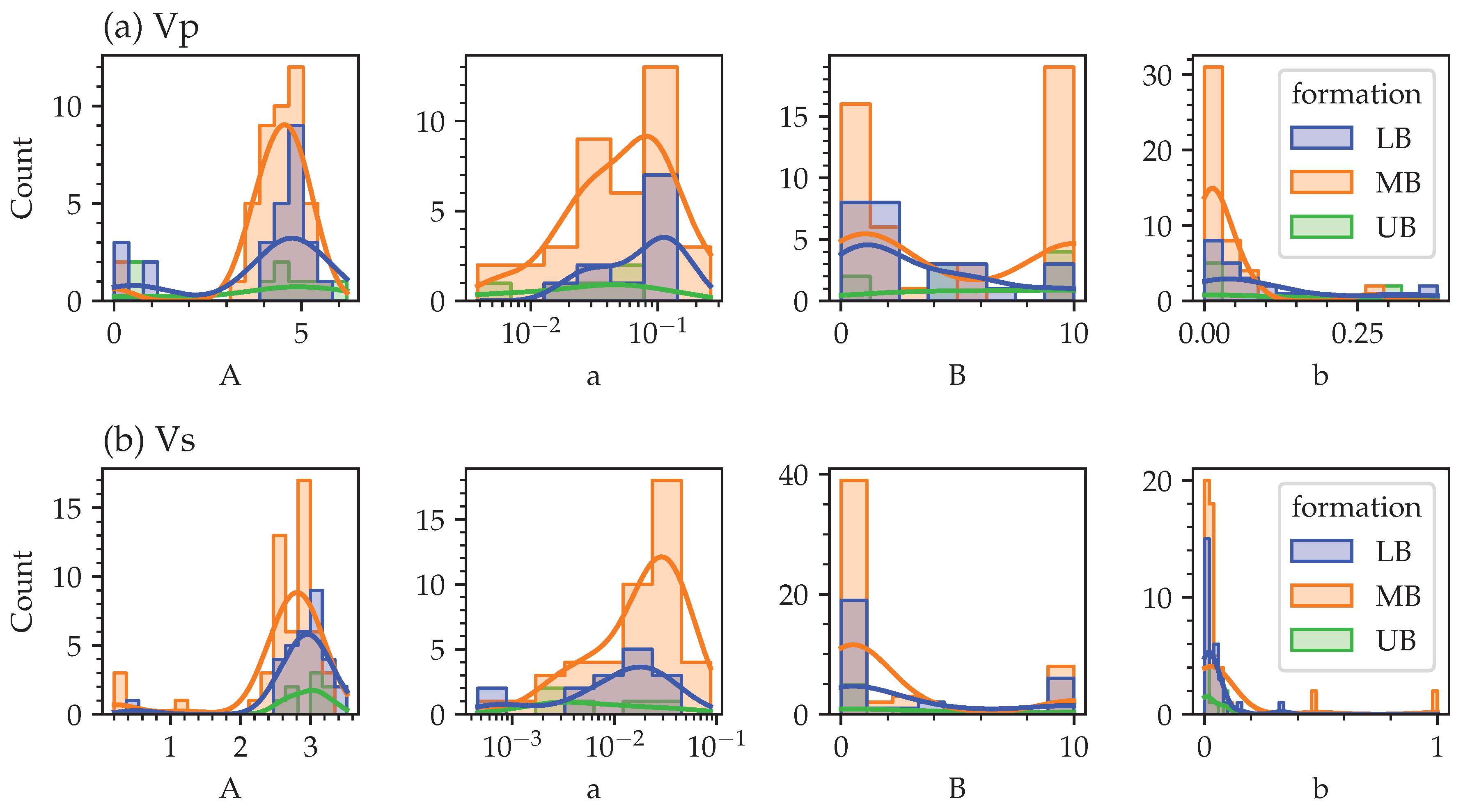
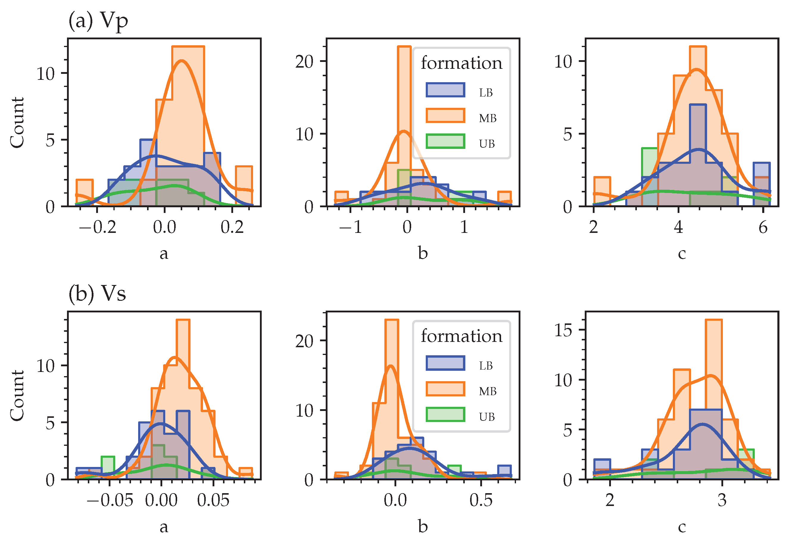
The superiority of Eberhart’s, Wepfer’s, and Wang’s models over a simple power function in fitting the data expands on the findings of prior research which have commonly used power functions for data estimation. This study hence proposes the use of these more sophisticated models for more accurate and reliable data fitting for the stress-sensitive elastic wave velocities evolution. This conclusion is corroborative with the previous studies [25]. Additionally, the observed model fitting evaluation metric suggests that the fitting of V s data is better than that of V p data.
The confining pressures applied on the core samples ranges from 10 to 50 MPa. The data results suggest that the points lie within the non-linear steep-rise section of the velocity–stress curve. In other words, the data may only represent the initial phase of the velocity–stress relationships, which is primarily governed by the effects of micro-cracks and pores [24]. Additional confining pressures are required to fully understand the velocity-effective relationships for the extended values of stress. We excluded samples from analysis where permeability increased or velocity decreased with confining pressure, as these indicate cracks or damage in the core samples.
Considering the mean parameters (A, K, B, and D) of Eberhart’s model presented in Table A1, we observed that an increment in effective confining stress from 0 to 50 MPa resulted in a 11.7% increase in V p for the LB formation, a 12.9% increase for the MB formation, and a 7.7% increase for the UB formation. Similarly, by taking into account the mean parameters (A, K, B, and D) of Eberhart’s model from Table A2, we found that a rise in effective confining stress from 0 to 50 MPa led to a 7.2% increase in V s for the LB formation, a 11.0% increase for the MB formation, and a 2.5% increase for the UB formation. Based on these observations, two significant conclusions can be drawn: (i) The increase in V p with rising effective stress is greater than that of V s . (ii) Among the formations studied, MB exhibits a higher sensitivity to stress variations compared to LB and UB formations. This percentage of increase is in the same range of the results obtained on limestone rocks [24], diorite, and gneiss rock types [34].
The evaluation metrics indicate that the power–law model performs better than the exponential model in fitting the measured permeability-effective stress data across all Bakken members. A similar observation was made in previous studies [38]. By examining the mean parameters of the power–law model (see Table A9) and the mean permeability values for each formation (see Table 1), we observe that a 50 MPa increase in net effective confining stress results in an 85% decrease in permeability for the Lower Bakken (LB), a 93% decrease for the Middle Bakken (MB), and a 77% decrease for the Upper Bakken (UB). Previous studies on the shale reservoir rocks display a similar order of permeability reduction with applied stress [14,48]. The net confining stress here is determined as the applied isotropic confining stress minus the pore pressure. However, caution should be exercised before concluding that the permeability of the MB formation is more stress-sensitive than that of the LB and UB due to the high variance in the fitting parameters and the relatively low sample size.
The contrast in model performance based on the geological formation (LB, MB, UB) correlates with the inherent geological variability across different layers of the Bakken formation, as illustrated in previous studies. The distinction in the variance of fitting parameters between LB, UB, and MB can be interpreted as a reflection of the geological complexity of these formations. The implications of the current study could serve as an important basis for further investigations into the influence of geological characteristics on model performance, especially considering the differential behavior of the LB and UB formations.
In this study, we have provided a comprehensive assessment of ultrasonic velocities and permeability changes under varying confining stress conditions. However, there are several crucial factors that necessitate consideration when interpreting the findings of this research and when incorporating them into future investigations. Firstly, the issue of sample size warrants attention. The number of core samples utilized for each geological formation can significantly impact the observed variance and mean values of fitting parameters. This has been emphasized in prior studies, highlighting the importance of maintaining a balanced sample size across different formations in order to ensure the reliability and robustness of the results. The stress range adapted in the current experiments may not represent the actual in situ stresses in the Bakken formation. Further experiments with extended confining stress will provide a complete spectrum of petrophysical properties evolution with stress.
Furthermore, the significant facies variance within each formation is a noteworthy aspect [3]. In order to achieve greater accuracy in the results, it is essential for future studies to explore modeling approaches that take into account geological facies variations within each formation.
The pronounced anisotropy of the Bakken members, particularly in the upper and lower sections due to thin shale laminations, is an important factor [46]. These thin laminations play a critical role in the elastic wave propagation and permeability characteristics of the rocks. Understanding such microstructural aspects, including pore morphology, clay distribution, grain arrangements, and other relevant factors, becomes crucial as they primarily dictate the petrophysical properties evolution in these rocks.
Hence, a comprehensive microstructural interpretation is imperative to gain deeper insights into the behavior of the rocks and their petrophysical properties. This understanding will further enhance our comprehension of ultrasonic velocities and permeability changes with varying confining stress and aid in advancing future research in this field.

Author Contributions

Conceptualization, P.P.; methodology, P.P.; software, P.P.; validation, P.P. and G.I.; formal analysis, P.P.; investigation, P.P.; resources, P.P. and K.L.; data curation, P.P. and K.L.; writing—original draft preparation, P.P. and K.L.; writing—review and editing, P.P., G.I. and K.L.; visualization, P.P.; supervision, K.L.; project administration, K.L.; funding acquisition, K.L. All authors have read and agreed to the published version of the manuscript.

Funding

This research received no external funding.

Data Availability Statement

All the information that supports the discoveries of this research is included in the article.

Acknowledgments

The authors would like to express and acknowledge the financial support of the North Dakota Industrial Commission (NDIC).

Conflicts of Interest

The authors declare no conflict of interest.

Nomenclature

The following abbreviations are used in this manuscript:
NDICNorth Dakota Industrial Commission
LBLower Bakken Member
MBMiddle Bakken Member
UBUpper Bakken Member
RRMSERelative Root Mean Square Error
σ e Effective Confining Stress
σ Total Confining Stress
σ i Initial Effective Confining Stress
P p Pore Pressure
kPermeability
ϕ Total Porosity
VCompressional or Shear Wave Velocity
V p Compressional Wave Velocity or Longitudinal Wave Velocity
V s Shear Wave Velocity or Transverse Wave Velocity
PcCritical Confining Pressure in Wang et al. (2005) [25] model
stdStandard Deviation of Gaussian Distribution

Appendix A

Appendix A.1

Table A1. Compressional wave velocity: Best fit parameters of the Eberhart-Phillips et al. (1989) [29] model.
FormationSizeAKBDRRMSE
MeanstdMeanstdMeanstdMeanstdMeanstd
LB265.2620.5260.4130.3330.7180.37812.67018.8067.6265.034
MB454.9760.3540.5470.4270.7090.32112.18619.9365.4204.111
UB95.2750.4520.4460.3840.6480.44111.8435.1668.0453.751
Table A2. Shear wave velocity: Best fit parameters of the Eberhart-Phillips et al. (1989) [29] model.
FormationSizeAKBDRRMSE
MeanstdMeanstdMeanstdMeanstdMeanstd
LB313.0730.3520.1210.1800.4610.38214.98515.9655.6705.984
MB533.1160.1710.0850.1840.4440.27116.16025.3303.4012.856
UB83.0350.2060.1100.1600.3710.40424.26819.5565.1343.330
Table A3. Compressional wave velocity: Best fit parameters of the Wepfer and Christensen (1991) [30] model.
FormationSizeAaBbRRMSE
MeanstdMeanstdMeanstdMeanstdMeanstd
LB263.9261.7500.1500.3193.2403.2200.1090.1267.2595.293
MB454.2951.0620.0080.0155.0724.4010.0300.0575.0133.787
UB94.0062.0420.2270.4386.3073.8140.0970.1277.6903.515
Table A4. Shear wave velocity: Best fit parameters of the Wepfer and Christensen (1991) [30] model.
FormationSizeAaBbRRMSE
MeanstdMeanstdMeanstdMeanstdMeanstd
LB312.8760.5050.0420.1782.8673.9060.0390.0646.7176.730
MB532.6200.6690.0480.1692.1453.4620.0820.2043.6623.267
UB82.9510.2620.0020.0032.8814.4530.0320.0385.4113.255
Table A5. Compressional wave velocity: Best fit parameters of the Wang et al. (2005) [25] model.
FormationSizeabcRRMSE
MeanstdMeanstdMeanstdMeanstd
LB26−0.0040.0900.2850.5714.3490.8687.1174.355
MB450.0480.096−0.0040.5384.3510.7705.4413.894
UB9−0.0310.0910.3790.5654.3721.0498.1123.374
Table A6. Shear wave velocity: Best fit parameters of the Wang et al. (2005) [25] model.
FormationSizeabcRRMSE
MeanstdMeanstdMeanstdMeanstd
LB31−0.0030.0260.1160.1872.7000.3066.1845.846
MB530.0180.0240.0040.1222.7660.2783.8632.926
UB8−0.0040.0290.0760.1912.8440.3905.6933.138
Table A7. Compressional wave velocity: Best fit parameters of the power function.
FormationSizevp0aRRMSE
MeanstdMeanstdMeanstd
LB264464.251493.8490.0490.03010.5135.523
MB454110.312566.1290.0520.0278.7234.830
UB94744.285548.5240.0320.01911.8514.834
Table A8. Shear wave velocity: Best fit parameters of the power function.
FormationSizevs0aRRMSE
MeanstdMeanstdMeanstd
LB312756.460203.4610.0300.0238.7216.787
MB532660.253269.8430.0350.0206.3243.094
UB82894.120228.5940.0160.0107.8073.739

Appendix B

Table A9. Best fit parameters of the power law and exponential models of permeability.
FormationSizebaRRMSE (Power)RRMSE (Exponential)
MeanstdMeanstdMeanstdMeanstd
LB10−1.2851.372−0.0590.0865.2813.1896.9233.730
MB8−1.8301.858−0.1710.3006.1773.1947.2034.404
UB2−1.165 −0.050 3.895 5.334

References

  1. Marra, K.R.; Mercier, T.J.; Gelman, S.E.; Schenk, C.J.; Woodall, C.A.; Cicero, A.D.; Drake, R.M., II; Ellis, G.S.; Finn, T.M.; Gardner, M.H.; et al. Assessment of Undiscovered Continuous Oil Resources in the Bakken and Three Forks Formations of the Williston Basin Province, North Dakota and Montana, 2021; Technical Report; US Geological Survey: Reston, VA, USA, 2021. [CrossRef]
  2. Pitman, J.K.; Price, L.C.; LeFever, J.A. Diagenesis and Fracture Development in the Bakken Formation, Williston Basin: Implications for Reservoir Quality in the Middle Member; The Bakken Formation as an Oil Resource; US Geological Survey: Reston, VA, USA, 2012; pp. 57–91.
  3. Simenson, A.L.; Sonnenberg, S.A.; Cluff, R.M. Depositional Facies and Petrophysical Analysis of the Bakken Formation, Parshall Field and Surrounding Area, Mountrail County, North Dakota. Master’s Thesis, Colorado School of Mines, Golden, CO, USA, 2011. Available online: http://hdl.handle.net/11124/16188 (accessed on 2 May 2023).
  4. Fatt, I.; Davis, D. Reduction in Permeability with Overburden Pressure. J. Pet. Technol. 1952, 4, 16. [Google Scholar] [CrossRef]
  5. Byerlee, J.D.; Zoback, M.D. Permeability and Effective Stress: Geologic Notes. AAPG Bull. 1975, 59, 154–158. [Google Scholar] [CrossRef]
  6. Li, W.; Frash, L.P.; Welch, N.J.; Carey, J.W.; Meng, M.; Wigand, M. Stress-dependent fracture permeability measurements and implications for shale gas production. Fuel 2021, 290, 119984. [Google Scholar] [CrossRef]
  7. Davies, J.P.; Davies, D.K. Stress-dependent permeability: Characterization and modeling. In Proceedings of the SPE Annual Technical Conference and Exhibition, Houston, TX, USA, 3–6 October 1999; pp. 429–444. [Google Scholar] [CrossRef]
  8. Zhou, X.; Zeng, Z.; Liu, H. Stress-dependent permeability of carbonate rock and its implication to CO2 sequestration. In Proceedings of the 45th US Rock Mechanics/Geomechanics Symposium, San Francisco, CA, USA, 26–29 June 2011. [Google Scholar]
  9. Meng, Z.; Zhang, J.; Wang, R. In-situ stress, pore pressure and stress-dependent permeability in the Southern Qinshui Basin. Int. J. Rock Mech. Min. Sci. 2011, 48, 122–131. [Google Scholar] [CrossRef]
  10. Lei, J.; Meng, Z.; Tan, L.; Wang, Y.; Wu, D. Experimental study on stress-dependent permeability of coal samples with different salinities of water in coal. Process Saf. Environ. Prot. 2023, 170, 403–414. [Google Scholar] [CrossRef]
  11. Bohnsack, D.; Potten, M.; Freitag, S.; Einsiedl, F.; Zosseder, K. Stress sensitivity of porosity and permeability under varying hydrostatic stress conditions for different carbonate rock types of the geothermal Malm reservoir in Southern Germany. Geotherm. Energy 2021, 9, 15. [Google Scholar] [CrossRef]
  12. Chen, T.; Feng, X.T.; Cui, G.; Tan, Y.; Pan, Z. Experimental study of permeability change of organic-rich gas shales under high effective stress. J. Nat. Gas Sci. Eng. 2019, 64, 1–14. [Google Scholar] [CrossRef]
  13. Cui, G.; Liu, J.; Wei, M.; Shi, R.; Elsworth, D. Why shale permeability changes under variable effective stresses: New insights. Fuel 2018, 213, 55–71. [Google Scholar] [CrossRef]
  14. Al Ismail, M.I.; Zoback, M.D. Effects of rock mineralogy and pore structure on stress-dependent permeability of shale samples. Philos. Trans. R. Soc. A Math. Phys. Eng. Sci. 2016, 374, 20150428. [Google Scholar] [CrossRef]
  15. Saurabh, S.; Harpalani, S.; Zakharova, N. Flow regime evolution and stress-dependent permeability in nanoporous rocks. Fuel 2022, 310, 122413. [Google Scholar] [CrossRef]
  16. Pothana, P.; Ifrene, G.; Ling, K.; Garcia, F.E. Investigating Grain Size Influence on the Stress-Dependent Permeability of Porous Rocks Using Particulate Discrete Element Method. In Proceedings of the U.S. Rock Mechanics/Geomechanics Symposium, Atlanta, GA, USA, 25–28 June 2023; p. ARMA-2023-0827. [Google Scholar] [CrossRef]
  17. Shi, J.Q.; Durucan, S.; Korre, A.; Ringrose, P.; Mathieson, A. History matching and pressure analysis with stress-dependent permeability using the In Salah CO2 storage case study. Int. J. Greenh. Gas Control 2019, 91, 102844. [Google Scholar] [CrossRef]
  18. Ali, T.A.; Sheng, J.J. Evaluation of the Effect of Stress-dependent Permeability On Production Performance in Shale Gas Reservoirs. In Proceedings of the SPE Eastern Regional Meeting, Morgantown, WV, USA, 13–15 October 2015; p. SPE-177299-MS. [Google Scholar] [CrossRef]
  19. Hatchell, P.; Bourne, S. Rocks under strain: Strain-induced time-lapse time shifts are observed for depleting reservoirs. Lead. Edge 2005, 24, 1222–1225. [Google Scholar] [CrossRef]
  20. Dvorkin, J.; Gutierrez, M.A.; Grana, D. Seismic Reflections of Rock Properties; Cambridge University Press: Cambridge, UK, 2014. [Google Scholar] [CrossRef]
  21. Holt, R.M.; Nes, O.M.; Fjaer, E. In-situ stress dependence of wave velocities in reservoir and overburden rocks. Lead. Edge 2005, 24, 1268–1274. [Google Scholar] [CrossRef]
  22. AutoLab 1500; New England Research Inc.: White River Junction, VT, USA, 2017.
  23. Pothana, P.; Gokapai, V.; Ifrene, G.; Ling, K. Effect of Binding Material on the Acoustic, Elastic and Strength Properties of Artificial Granular Rocks. In Proceedings of the 2023 All Days U.S. Rock Mechanics/Geomechanics Symposium, Atlanta, GA, USA, 25–28 June 2023; p. ARMA-2023-0560. [Google Scholar] [CrossRef]
  24. Asef, M.R.; Najibi, A.R. The effect of confining pressure on elastic wave velocities and dynamic to static Young’s modulus ratio. Geophysics 2013, 78, D135–D142. [Google Scholar] [CrossRef]
  25. Wang, Q.; Ji, S.; Salisbury, M.H.; Xia, B.; Pan, M.; Xu, Z. Pressure dependence and anisotropy of P-wave velocities in ultrahigh-pressure metamorphic rocks from the Dabie–Sulu orogenic belt (China): Implications for seismic properties of subducted slabs and origin of mantle reflections. Tectonophysics 2005, 398, 67–99. [Google Scholar] [CrossRef]
  26. Hardin, B.O.; Richart, F., Jr. Elastic wave velocities in granular soils. J. Soil Mech. Found. Div. 1963, 89, 33–65. [Google Scholar] [CrossRef]
  27. Kopperman, S.E.; Stokoe, K.H., II; Knox, D.P. Effect of State of Stress on Velocity of Low-Amplitude Compression Waves Propagating along Principal Stress Directions in Dry Sand; Technical Report; United States Air Force, Office of Scientific Research, Boiling Air Force Base: Washington, DC, USA, 1982.
  28. Guerriero, V.; Mazzoli, S. Theory of Effective Stress in Soil and Rock and Implications for Fracturing Processes: A Review. Geosciences 2021, 11, 119. [Google Scholar] [CrossRef]
  29. Eberhart-Phillips, D.; Han, D.H.; Zoback, M. Empirical relationships among seismic velocity, effective pressure, porosity, and clay content in sandstone. Geophysics 1989, 54, 82–89. [Google Scholar] [CrossRef]
  30. Wepfer, W.; Christensen, N. A seismic velocity-confining pressure relation, with applications. Int. J. Rock Mech. Min. Sci. Geomech. Abstr. 1991, 28, 451–456. [Google Scholar] [CrossRef]
  31. Castagna, J.P.; Batzle, M.L.; Eastwood, R.L. Relationship between Compressional and Shear-Wave Velocities in Classic Silicate Rocks; SEG Technical Program Expanded Abstracts 1984; Society of Exploration Geophysicists: Houston, TX, USA, 1984; pp. 582–584. [Google Scholar] [CrossRef]
  32. Qin, X.; Han, D.h.; Zhao, L. Rock Physics Modeling of Organic-Rich Shales with Different Maturity Levels; SEG Technical Program Expanded Abstracts 2014; Society of Exploration Geophysicists: Houston, TX, USA, 2014; Volume 33, pp. 2952–2957. [Google Scholar] [CrossRef]
  33. David, C.; Wong, T.f.; Zhu, W.; Zhang, J. Laboratory measurement of compaction-induced permeability change in porous rocks: Implications for the generation and maintenance of pore pressure excess in the crust. Pure Appl. Geophys. 1994, 143, 425–456. [Google Scholar] [CrossRef]
  34. Chen, D.; Pan, Z.; Ye, Z.; Hou, B.; Wang, D.; Yuan, L. A unified permeability and effective stress relationship for porous and fractured reservoir rocks. J. Nat. Gas Sci. Eng. 2016, 29, 401–412. [Google Scholar] [CrossRef]
  35. Shi, Y.; Wang, C.Y. Pore pressure generation in sedimentary basins: Overloading versus aquathermal. J. Geophys. Res. 1986, 91, 2153. [Google Scholar] [CrossRef]
  36. Nolte, S.; Fink, R.; Krooss, B.M.; Littke, R. Simultaneous determination of the effective stress coefficients for permeability and volumetric strain on a tight sandstone. J. Nat. Gas Sci. Eng. 2021, 95, 104186. [Google Scholar] [CrossRef]
  37. Zhang, S.; Sang, Q.; Dong, M. Experimental study of pressure sensitivity in shale rocks: Effects of pore shape and gas slippage. J. Nat. Gas Sci. Eng. 2021, 89, 103885. [Google Scholar] [CrossRef]
  38. Ghabezloo, S.; Sulem, J.; Guédon, S.; Martineau, F. Effective stress law for the permeability of a limestone. Int. J. Rock Mech. Min. Sci. 2009, 46, 297–306. [Google Scholar] [CrossRef]
  39. Dong, J.J.; Hsu, J.Y.; Wu, W.J.; Shimamoto, T.; Hung, J.H.; Yeh, E.C.; Wu, Y.H.; Sone, H. Stress-dependence of the permeability and porosity of sandstone and shale from TCDP Hole-A. Int. J. Rock Mech. Min. Sci. 2010, 47, 1141–1157. [Google Scholar] [CrossRef]
  40. Egenhoff, S. The lost Devonian sequence—Sequence stratigraphy of the middle Bakken member, and the importance of clastic dykes in the lower Bakken member shale, North Dakota, USA. Mar. Pet. Geol. 2017, 81, 278–293. [Google Scholar] [CrossRef]
  41. Sonnenberg, S.A. The Bakken–Three Forks super giant play, Williston Basin. AAPG Bull. 2020, 104, 2557–2601. [Google Scholar] [CrossRef]
  42. Pollastro, R.M.; Roberts, L.N.; Cook, T.A. Geologic Assessment of Technically Recoverable Oil in the Devonian and Mississippian Bakken Formation, Chap. 5 of U.S. Geological Survey Williston Basin Province Assessment Team, Assessment of Undiscovered Oil and Gas Resources of the Williston Basin Province of North Dakota, Montana, and South Dakota, 2010; version 1.1, November 2013; U.S. Geological Survey Digital Data Series DDS-69-W; U.S. Geological Survey: Reston, VA, USA, 2013; 34p.
  43. Scott Hamlin, H.; Smye, K.; Dommisse, R.; Eastwood, R.; Lemons, C.R.; McDaid, G. Geology and petrophysics of the bakken unconventional petroleum system. In Proceedings of the SPE/AAPG/SEG Unconventional Resources Technology Conference 2017, Austin, TX, USA, 24–26 July 2017; pp. 1294–1307. [Google Scholar] [CrossRef]
  44. Simpson, G.; Hohman, J.; Pirie, I.; Horkowitz, J. Using Advanced Logging Measurements to Develop a Robust Petrophysical Model for the Bakken Petroleum System. In Proceedings of the All Days SPWLA Annual Logging Symposium 2015, Long Beach, CA, USA, 18–22 July 2015; Available online: https://onepetro.org/SPWLAALS/proceedings-pdf/SPWLA15/All-SPWLA15/SPWLA-2015-Z/1342505/spwla-2015-z.pdf (accessed on 2 May 2023).
  45. Ramiro-Ramirez, S.; Flemings, P.B.; Bhandari, A.R.; Jimba, O.S. Steady-State Liquid Permeability Measurements in Samples from the Bakken Formation, Williston Basin, USA. In Proceedings of the SPE Annual Technical Conference and Exhibition, Dubai, United Arab Emirates, 21–23 September 2021. [Google Scholar] [CrossRef]
  46. Ostadhassan, M. Geomechanics and Elastic Anisotropy of the Bakken Formation, Williston Basin. Ph.D. Thesis, University of North Dakota, Grand Forks, ND, USA, 2013. Available online: https://commons.und.edu/theses/219 (accessed on 2 May 2023).
  47. Arns, C.H.; Knackstedt, M.A.; Pinczewski, W.V. Accurate Vp:Vs relationship for dry consolidated sandstones. Geophys. Res. Lett. 2002, 29, 44-1–44-4. [Google Scholar] [CrossRef]
  48. Teklu, T.W.; Li, X.; Zhou, Z.; Abass, H. Experimental investigation on permeability and porosity hysteresis of tight formations. SPE J. 2018, 23, 672–690. [Google Scholar] [CrossRef]
Figure 1. Autolab-1500 equipment (left) and the schematic (right) showing the key components of the pressurization system. Modified after [23].
Fuels 04 00025 g001
Figure 2. Schematic diagram showing various V p -effective stress empirical models [25,26,29,30].
Fuels 04 00025 g002
Figure 3. Schematic stratigraphic cross-section of the Devonian–Mississippian Bakken Formation, depicting Lower Bakken, Middle Bakken, and Upper Bakken members and the Bakken composite continuous reservoir (modified after [42]).
Fuels 04 00025 g003
Figure 4. Statistical distribution of the porosity, permeability, V p , and V s (from left to right) corresponding to the LB, MB, and UB. The distribution corresponding to the three Bakken members LB, MB, and UB are represented in blue, orange, and green colors respectively.The width of the violin plot is proportional to the count of the histograms.
Fuels 04 00025 g004
Figure 5. Velocity-effective stress plots: (a) Longitudinal wave velocity ( V p ) versus net-effective stress for the LB, MB, and UB. (b) Transverse wave velocity ( V s ) versus net-effective stress for the LB, MB, and UB.
Fuels 04 00025 g005
Figure 6. Distribution of best fit parameters of Power Model (a) V p and (b) V s . The fitting parameters “Vi” and “a” are defined in Equation (1). The distribution corresponding to the three Bakken members LB, MB, and UB are represented in blue, orange, and green colors. The solid lines overlapping the histograms represents kernel density estimation (KDE).
Fuels 04 00025 g006
Figure 7. Distribution of best fit parameters of Eberhart-Phillips et al. (1989) [29] model (a) V p and (b) V s . The fitting parameters “A”, “K”, “B”, and “D” are defined in Equation (3). The distribution corresponding to the three Bakken members LB, MB, and UB are represented in blue, orange, and green colors. The solid lines overlapping the histograms represent KDE smoothed values.
Fuels 04 00025 g007
Figure 8. Distribution of best fit parameters of Wepfer and Christensen (1991) [30] model (a) V p and (b) V s . The fitting parameters A, a, B, and b are defined in Equation (4). The distribution corresponding to the three Bakken members LB, MB, and UB are represented in blue, orange, and green colors. The solid lines overlapping the histograms represents KDE smoothed values.
Fuels 04 00025 g008
Figure 9. Distribution of best fit parameters of Wang et al. (2005) [25] model (a) V p and (b) V s . The fitting parameters a, b and c are defined in the Equation (6). The distribution corresponding to the three Bakken members LB, MB, and UB are represented in blue, orange, and green colors. The solid lines overlapping the histograms represents KDE smoothed values.
Fuels 04 00025 g009
Figure 10. Compressional and shear wave velocity correlations.
Fuels 04 00025 g010
Figure 11. V s prediction from V p using the well log data. (From left) The first track represents depth, Gamma Ray (GR) measurements are presented in the second track, resistivity data are presented in the third track, bulk density and neutron porosity are presented in the fourth track, log measured compressional wave velocities (V_P) and core-derived compressional velocities (V_P_core) are presented in fifth track, and log measured shear wave velocity (V_S), core measured shear wave velocity (V_S_core), and predicted shear wave velocity using the model (VS_MODEL) are presented in sixth track.
Fuels 04 00025 g011
Figure 12. Permeability evolution data with effective stress in three formations LB, MB, and UB.
Fuels 04 00025 g012
Figure 13. Best fit parameters of the power–law and exponential models of the permeability-effective stress. The distribution corresponding to the three Bakken members LB, MB, and UB are represented in blue, orange, and green colors. The solid lines overlapping the histograms represents KDE smoothed values. (b) represents the fitting parameter of the power law model. (a) represents the fitting parameter of the exponential model.
Fuels 04 00025 g013
Table 1. Statistical summaries of the porosity, permeability, V p , and V s .
FormationPermeability ( µ D)Porosity (%)Vp (m/s)Vs (m/s)
CountMeanstdCountMeanstdCountMeanstdCountMeanstd
LB511185.683848.31585.691.33374895.92415.88372921.68218.92
MB121127.47672.831394.791.38534645.94501.22532843.92194.55
UB336613.2410,551.83404.272.09105103.10484.02103014.50197.67
std = Standard Deviation of Gaussian Distribution.
Disclaimer/Publisher’s Note: The statements, opinions and data contained in all publications are solely those of the individual author(s) and contributor(s) and not of MDPI and/or the editor(s). MDPI and/or the editor(s) disclaim responsibility for any injury to people or property resulting from any ideas, methods, instructions or products referred to in the content.

