
Nonlinear Modeling of an Automotive Air Conditioning System Considering Active Grille Shutters

Department of Mechanical, Automotive & Materials Engineering, University of Windsor, 401 Sunset Ave, Windsor, ON N9B 3P4, Canada
*
Author to whom correspondence should be addressed.
Modelling 2023, 4(1), 70-86; https://doi.org/10.3390/modelling4010006
Submission received: 7 December 2022
/
Revised: 20 January 2023
/
Accepted: 29 January 2023
/
Published: 2 February 2023
Abstract
:This paper expands upon the state of the art in nonlinear modeling of automotive air conditioning systems. Prior models considered only the effects of the refrigerant compressor and the condenser fan. There are two new aspects included here. First, we create a mathematical model for front-end underhood airflow, considering vehicle speed, condenser fan rotational speed, and active grille shutter position. In addition, we present a new model for the power consumption of the vehicle associated with aerodynamic drag caused by underhood flow, as well as a fan power model which accounts not only for changes in rotational speed but also changes in flow rate. The models developed in this paper are coded in MATLAB/Simulink and assessed for various vehicle driving conditions against a higher-fidelity vehicle energy management model, showing good agreement. By including the active grille shutters as a controllable actuator and the impact of underhood flow on vehicle drag and fan power consumption, control schemes can be developed to holistically target reduced energy consumption for the air conditioning system and, thus, improve the overall vehicle energy efficiency.
1. Introduction
Automotive air conditioning (A/C) systems are often modeled mathematically to demonstrate the performance and behavior of their components as the system attempts to cool the vehicle’s cabin. State-of-the-art models for A/C systems consider the compressor and condenser fan as controllable actuators to maintain cabin comfort. In work published to date, consideration of the active grill shutters (AGS) as a controllable actuator is not present [1,2,3]. The AGS impacts the cooling performance of the A/C system, as it provides an additional mechanism to control airflow through the condenser at a given vehicle speed in addition to the fan rotational speed [4,5]. The amount of underhood flow also affects vehicle drag, which can be accounted for via the power consumption of the A/C system [6,7]. Many mathematical models of A/C systems are developed with the intention of control implementation, with the reduction in energy consumption considered a primary objective [8]. Most models used by controllers in academic literature only consider the compressor and condenser fan as controllable actuators since those have a high power consumption [9,10]. The model presented in this paper builds upon the state of the art by introducing the AGS as a controllable actuator to regulate the front-end airflow, and considers the underhood vehicle airflow drag effects on the power consumption of the vehicle. This paper thus presents a holistic model for the automotive A/C system power consumption.
The novelty of this work is in extending an A/C system model’s completeness by considering front-end airflow cooling effects and power consumption comprising of:
- Improving the completeness of the vehicle A/C nonlinear model by adding the impact of the AGS on the determination of the underhood airflow;
- Developing a holistic model for the A/C system power consumption by considering underhood aerodynamic drag effects;
- Creating a fan power consumption model that captures the impact of changing rotational speed and volumetric airflow rate.
It must be emphasized that the contribution of this paper is less about the specific NL model developed, which is, of course, only applicable to one particular vehicle. Instead, the approach outlined is the contribution, as this could be applied to any vehicle, regardless of whether the source of reference data is a vehicle energy management (VEM) model or experimental measurements made on-vehicle.
The remaining sections of this paper are organized as follows. Section 2 outlines the details of the system being modeled, the underlying mathematical model used to develop the extended model formulated in this work, and the new advancements to previous modeling work described in the literature [11]. Section 3 includes the validation of the nonlinear (NL) model with the higher-fidelity VEM model, an analysis of the holistic power consumption model, a demonstration of the nonlinear model’s ability to react to imposed step inputs, and a discussion of the results.
In this paper, several models are referenced throughout. In order to maintain clarity and consistency, a short summary and comparison of the two models are introduced in Table 1. The NL model is created by extending the modeling work carried out in [11], namely by creating curve fit approximations for refrigerant properties, developing models for compressor, fan, and drag power consumption, introducing tuning parameters to account for Nusselt number modeling uncertainty, and developing a model for the underhood airflow calculation based on the fan speed, AGS position, and vehicle speed, which is detailed in Section 3. In this paper, the NL model is implemented in Simulink. The VEM model in this paper is a high-fidelity model developed by the industrial partner for the purpose of simulating a virtual vehicle for various driving conditions. In this paper, the NL and VEM models are both simulated for the same driving conditions, discussed in Section 3. The results are compared to observe how well the NL model matches the behavior of the VEM model.
2. Materials and Methods
2.1. Description of A/C System Model
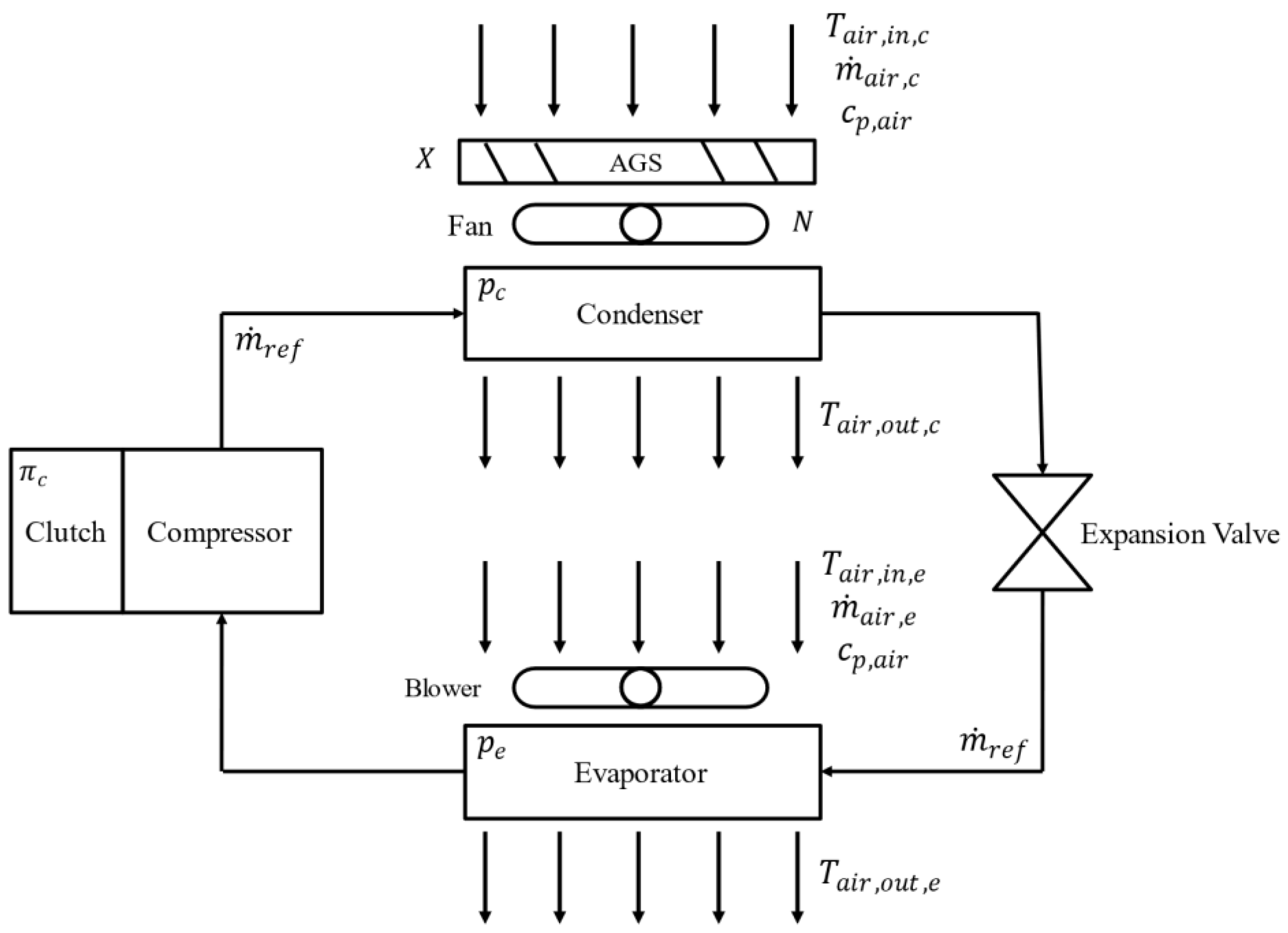
Figure 1 depicts a simplified block diagram of the A/C system, showcasing the connection of components, the flow of air and refrigerant, and the mathematical variables discussed in the underlying mathematical model of the system in Section 2.4.
The four main components along the A/C system’s refrigerant loop are the compressor, condenser, expansion valve, and evaporator. To develop a complete model of the A/C system, component models must capture the behavior of these four components. This paper describes such a model for implementing a controller for reducing energy consumption in future work. The controller will regulate the system to send the correct air temperature to the cabin while minimizing the power consumption of the A/C system. The heat exchanger (HEX) pressures are the minimum quantities needed to fully describe the behavior of this system and are chosen as the state variables. The model thus is formed as:
where and are the refrigerant pressures in the condenser and evaporator, is the compressor clutch engagement (on/off), is the rotational speed of the condenser fan, is the open-fraction of the AGS, is the refrigerant mass flow rate, is the volume flow rate of the air from the blower fan, and are the inlet air temperatures to the condenser and evaporator, is the inlet enthalpy to the condenser, and is the vehicle speed. Models for and based on the behavior of the refrigerant are described in Section 2.4. Since the intended usage of the model is within a control scheme to reach the target cabin temperature with minimum energy consumption, we also develop models of the energy consumption of the overall A/C system, including additional drag due to underhood flow, in Section 2.7. The inclusion of the impact of the AGS on underhood airflow and of the increase in power consumption associated with drag caused by that underhood flow are the key advancements over the state of the art presented in this paper.
2.2. Reference System
The ultimate intended use of the NL model is within control frameworks that require an analytical plant model. However, the application to control is outside the scope of this paper. The VEM model has been developed and validated by the industrial partner using experimental data gathered from testing on the real physical vehicle. The industrial partner’s VEM model has been developed under best practices from the literature [13,14]. In this paper, the VEM model acts as a substitute for an actual physical vehicle for controller development; the output from the VEM model is treated as the output from the physical vehicle. Thus, the nonlinear models in this paper are validated against the VEM model. Recall that the focus is on the approach, which is general, rather than the specifics of the VEM and NL models, which are specific to a particular vehicle. The reference system could just as easily be measured data from a vehicle; this would have no impact on the development, tuning, and assessment of the NL model.
2.3. Compressor
The VEM model includes a model of the A/C compressor. The VEM model uses the current baseline production controls to determine the compressor displacement, then provides a mass flow rate and outlet enthalpy value at each time step throughout the drive cycle. Since the NL model is meant to be used as a plant model within a control scheme, it is not necessary to model the compressor since the outputs are directly available from the plant (physical vehicle or VEM model representation).
2.4. Heat Exchangers
The two HEXs in the A/C system are the condenser and evaporator, where the refrigerant undergoes phase changes between liquid and vapor states. The mathematical models of these two HEXs must capture this change in thermodynamic state. The underlying HEX mathematical equations were derived from first principles and provided by the industrial partner based on work described in [11]. The work in [11] provides a simplified method to obtain a mathematical model for the HEX pressure by assuming a two-phase flow (liquid and gaseous) and approximating the thermodynamic states at the inlet and outlet of each HEX by relating it to the saturated liquid and vapor conditions. At the condenser outlet, the refrigerant is a saturated liquid. At the evaporator inlet, the refrigerant is assumed to have the same enthalpy as the refrigerant at the condenser outlet. The pressure at the inlet and outlet of the evaporator are equal, with a 10 °C superheat at the evaporator outlet maintained by the expansion valve. This will be further discussed in Section 2.5. The full derivation of the nonlinear pressure equations is available in [11], which results in the final forms:
where is the volume flow rate of the air through the condenser, is the air density, is the outlet refrigerant enthalpy, is the outlet air temperature, are the densities and enthalpies for the refrigerant calculated at saturated liquid and vapor states, is the specific heat of the HEX material, is the specific heat of air at constant pressure, is the mean void fraction of the refrigerant, is the volume of the HEX, is the material mass of the HEX, and is the wall temperature of the HEX. The constant values for the HEX and fluid properties are detailed in Appendix A. The derivation of polynomial models for the refrigerant thermodynamic properties is detailed in Section 2.6.
The second main aspect of this NL model is the temperature of the air leaving the evaporator, which is sent to the cabin for cooling. The air temperature depends on the temperature difference between the refrigerant temperature and air temperature passing through the evaporator, as well as the Nusselt number. A general model for the temperature of the air exiting a heat exchanger (condenser/evaporator) is given by:
where is the HEX refrigerant temperature and is the number of transfer units of the air. The final model of the air temperature in [11] is:
where is the convective heat transfer coefficient of the air, is the external surface area of the HEX, is the fraction of air-to-structure surface area on the fins, is the air-side fin efficiency, is the mass flow rate of the air, and and act as multipliers on the Nusselt number. As stated earlier, the derivation of polynomial models for the refrigerant thermodynamic properties, such as and , are detailed in Section 2.6.
The industrial partner provided computational fluid dynamics (CFD) data related to the specific vehicle of interest for this project, which included airflow rate values measured at various combinations of vehicle speed, fan rotational speed, and AGS open-fraction. A multiple linear regression method was used to create a model for the condenser airflow rate function based on these data.
A second-order regression model is the simplest model order that makes sense physically. A linear model would have three terms: one each for the AGS open-fraction, fan rotational speed, and vehicle speed. When the fan speed and vehicle speed are zero, the linear AGS term will cause a nonzero flow rate to be predicted by the model, which does not make sense physically, so the model does not include a linear AGS term. Thus, a second-order model with cross terms is the simplest model able to include the effect of all three inputs affecting the airflow. The second-order model provided a good fit to the data, with an value of 0.9981. Model orders higher than two were created and tested, but none provided a significant improvement to the goodness of fit to the data; thus, a model order of two was used.
The model takes the form:
where is the volume flow rate of the air in , is the normalized rotational speed of the condenser fan between zero and one, is the open-fraction of the AGS between zero and one, and the vehicle speed, , is in .
2.5. Expansion Valve
As mentioned previously, the thermodynamic states at the inlet and outlet of the HEXs are approximated based on the saturated liquid and vapor states. A similar assumption was introduced in [11] for modeling the expansion valve. The expansion valve regulates the refrigerant superheat temperature at the exit of the evaporator using a sensing bulb to maintain a constant superheat of 10 °C to the refrigerant at the evaporator exit. This means the refrigerant conditions at the evaporator exit can be related to the saturated conditions of the refrigerant pressure level inside the evaporator. The modeling approach used in [11] also assumes that the enthalpy at the inlet of the evaporator is equal to the enthalpy at the outlet of the condenser, meaning there is no heat loss across the expansion valve.
2.6. Refrigerant Temperature
In this paper, to model the thermodynamic properties of the refrigerant, a linear least-squares regression method was used to fit continuous curves to discrete refrigerant property data from [15]. The range of pressure data used for the curve fitting is equal to the standard operating range of each HEX, as defined by the industrial partner. An example of one of the resulting polynomial models is:
where is the temperature of the refrigerant leaving the condenser and is the condenser refrigerant pressure. The full list of fitted curves is presented in Appendix A in Equations (A1)–(A4). As mentioned earlier, this modeling work is intended for controller development. In this case, these polynomial curves must retain their accuracy when linearized for linear control approaches. When conducting curve fitting to a data set, the possibility of large oscillations occurring at either side of a discrete data point increases as the order of the polynomial increases. This is called Runge’s phenomenon [16]. To ensure that this problem does not arise for this model, the first derivative was compared with the numerical first differences between data points. Using polynomial functions instead of lookup tables results in less effort during the linearization of the model to compute the derivatives. This is due to the fact that the derivatives of lookup tables may be unavailable for discrete data sets. After replacing the lookup tables with the polynomial equations, the root mean squared error (RMSE) for the system output had only a 0.1 °C increase. The RMSE definition used for this purpose is formed as:
where is the variable value from the data, is the variable value from the model, and is the total number of data points. To assess the impact of this change, the RMSE was normalized using the range of the data set, resulting in a normalized RMSE of 0.19%.
2.7. Power Consumption
The control design that will use this model will be utilized to reduce the power consumption of the A/C system. Thus, a model of the power-consuming aspects must be defined as well, that being the compressor, condenser fan, and power consumption due to aerodynamic drag associated with the underhood airflow. The compressor’s power consumption is modeled from first principles using well-established thermodynamic and mechanical relationships from [17]. For brevity, the final form of the equation is given as:
where is the mass flow rate of the refrigerant, and are the enthalpies of the refrigerant at the inlet and outlet of the compressor, and is the ratio of isentropic efficiency to volumetric efficiency of the compressor.
The power consumption of the condenser fan is computed based on the underhood airflow and work done by the fan. From the Euler turbine equation, this is:
where is the power consumption of the fan and is the stagnation enthalpy change across the fan. The enthalpy change across the fan is not explicitly known, but data have been provided by the industrial partner for the fan pressure rise and adiabatic efficiency. For the low-speed incompressible flow of a perfect gas, the stagnation enthalpy change can be expressed in terms of the fan pressure rise and efficiency:
where is the pressure rise required of the fan and is the fan adiabatic efficiency. Substituting this expression into Equation (9) yields the final form of the fan power equation:
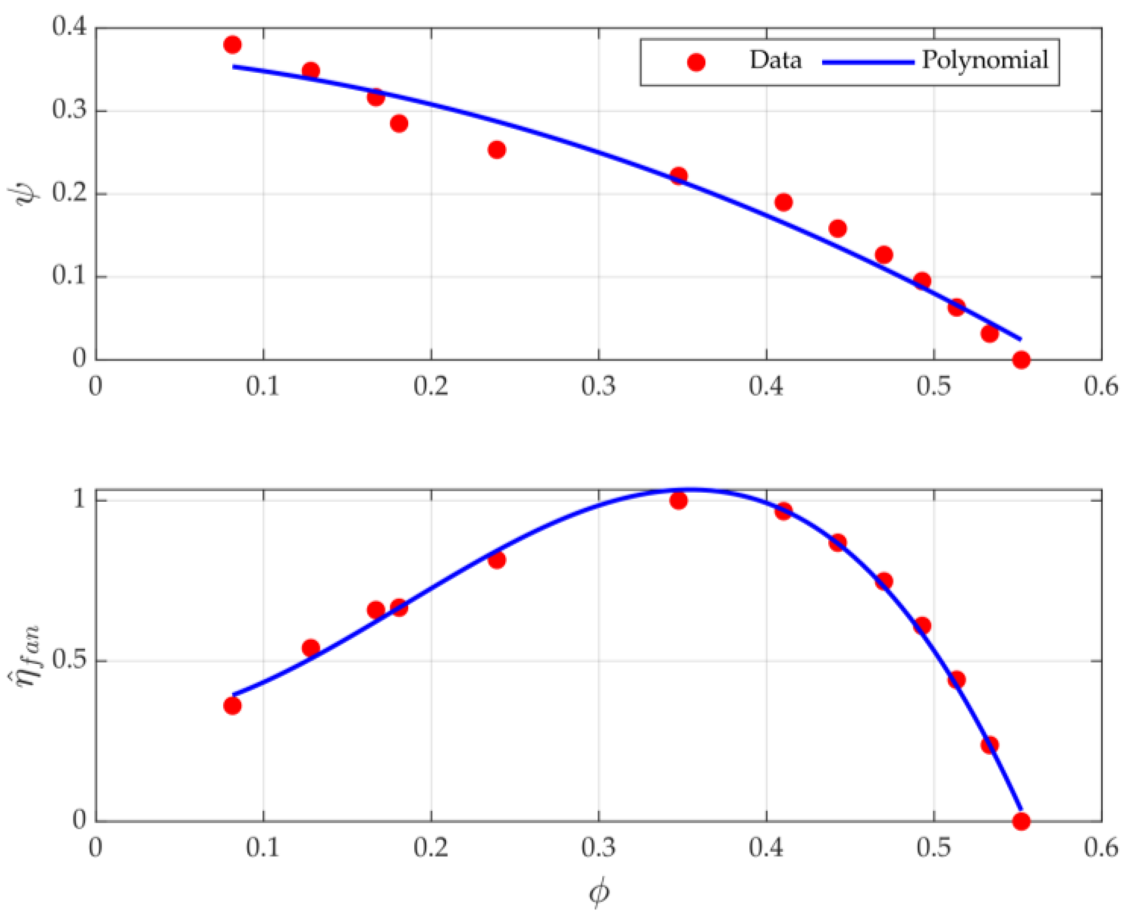
Recall that a model for has been established and is given by Equation (5). Thus, analytical expressions are needed for the fan pressure rise and efficiency to complete this fan power model. The industrial partner supplied experimental data for the fan pressure rise and efficiency at various underhood airflow rates for a fan speed of 2500 rpm. A relationship between the underhood airflow rate, fan pressure rise, and efficiency can be determined from these data, but it is only valid when the fan speed is at 2500 rpm. For this model, the flow is assumed to be incompressible. We neglect the effect of Reynolds number variations on efficiency and pressure rise. To enable the scaling of the power consumption model for any fan rotational speed, the pressure rise and airflow data were nondimensionalized to convert the experimental data from dimensional pressure rises and flow rates to nondimensional pressure rise coefficients and flow coefficients. These nondimensional parameters are expressed as:
where is the flow coefficient, is the pressure rise coefficient, and are the axial and midspan blade speeds, is the cross-sectional flow area of the fan, is the rotational speed of the fan in rotations per minute, and is the midspan radius of the fan. Two polynomial equations were developed using a least-squares regression method to fit polynomial equations to the nondimensionalized experimental data, shown in Figure 2. In Figure 2, the fan efficiency has been normalized using the highest fan efficiency provided in the experimental data.
These two polynomials relate the pressure rise coefficient and the efficiency of the fan to the flow coefficient of the underhood airflow and are given by:
The equations are valid for . In this range, the maximum error for the pressure rise coefficient is 0.034 (13.5%), and the maximum error for the efficiency is 5.4%. The pressure rise coefficient and efficiency are found using the expressions above after nondimensionalizing the flow rate. Next, the pressure rise is calculated by dimensionalizing the pressure rise coefficient and used with the efficiency and dimensional flow rate in Equation (11) to calculate the fan power.
As an extension to the previous modeling work from [11], a model was created to evaluate the power consumption associated with additional drag on the vehicle due to underhood airflow, which is set by the vehicle speed, fan rotational speed, and AGS open-fraction. The model for this power consumption is:
where is the frontal area of the vehicle and is the increase in drag coefficient due to additional flow through the underhood at a given vehicle speed due to the AGS being open and/or the fan being on.
To create a model for the drag coefficient, the industrial partner supplied experimental data for the drag coefficient as a function of underhood air volume flow rate at a constant vehicle speed of 67 mph. Since the data for the drag coefficient were only available for a single vehicle speed, the model for the underhood air volume flow rate in Equation (5) was normalized using the vehicle speed. The weak impact of vehicle speed on the flow rate can be observed by dividing Equation (5) by . A linear least-squares regression method was used to create a polynomial fit for the drag coefficient as a function of the normalized flow rate from the experimental data:
where the RMSE is 0.000419. As mentioned earlier, the increase in the drag coefficient relative to the flow rate achieved when the AGS is closed and the fan is off is computed and used in Equation (14) to calculate the additional power required due to the increase in drag on the underhood of the vehicle.
2.8. Model Implementation
To implement the NL model in MATLAB/Simulink, drive cycle parameters and initial conditions were coded in MATLAB to create a set of input parameters to simulate the model. The drive cycle parameters include the vehicle speed profile, ambient air conditions, etc. Equations (2) and (4) are implemented in Simulink to create a model of the A/C system. A subsystem model for each HEX was created with its specific equation outlined in Equations (2) and (4), along with the HEX physical properties to fully recreate the mathematical expressions shown in Equations (2) and (4). The thermodynamic state of the refrigerant at the outlet of the condenser model is sent directly to the evaporator model to be used as inputs. The VEM model is connected in place of a compressor model, and the former sends the compressor outputs to Simulink. The MATLAB script initializes the drive cycle conditions, then executes the NL model in Simulink and records the results.
2.9. Heat Exchanger Multiplier Parameter Calibration
As mentioned, there can be significant uncertainty in modeling the convective heat transfer and Nusselt number. The Nusselt number was tuned for each HEX by adding a coefficient, denoted as and for the condenser and evaporator, respectively. A grid search method was used to find the combination of coefficient values that reduced the RMSE for the NL model output, which is the air temperature leaving the evaporator, . This optimization yielded a minimum normalized RMSE value of 3.4%, with a value of 0.29 and a value of 0.55. The normalized RMSE was calculated by dividing the RMSE found using Equation (7) by the air temperature range. This is an improvement from the normalized RMSE of the original model in [11] (with no multipliers) of 5.4%.
3. Results and Discussion
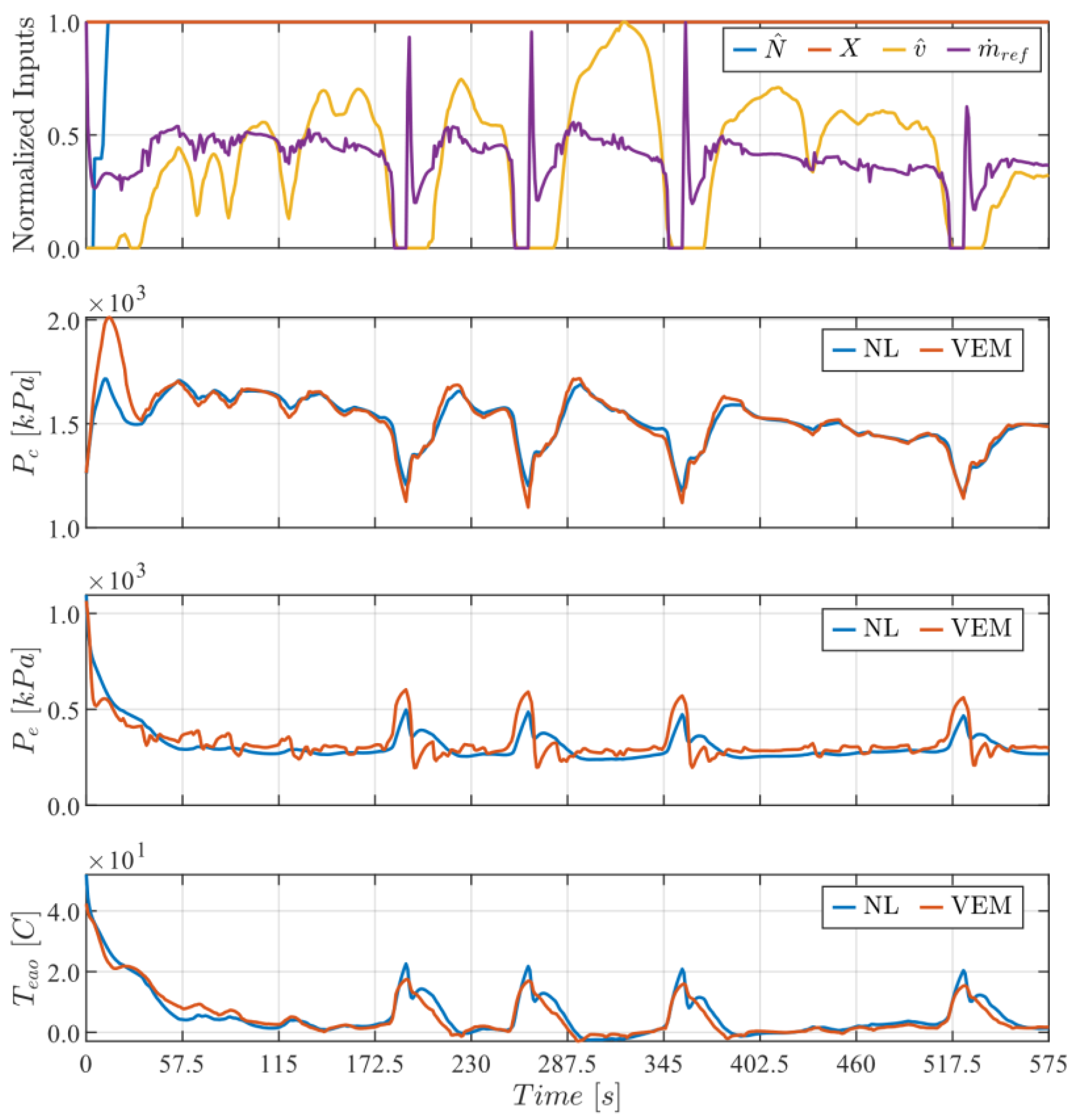
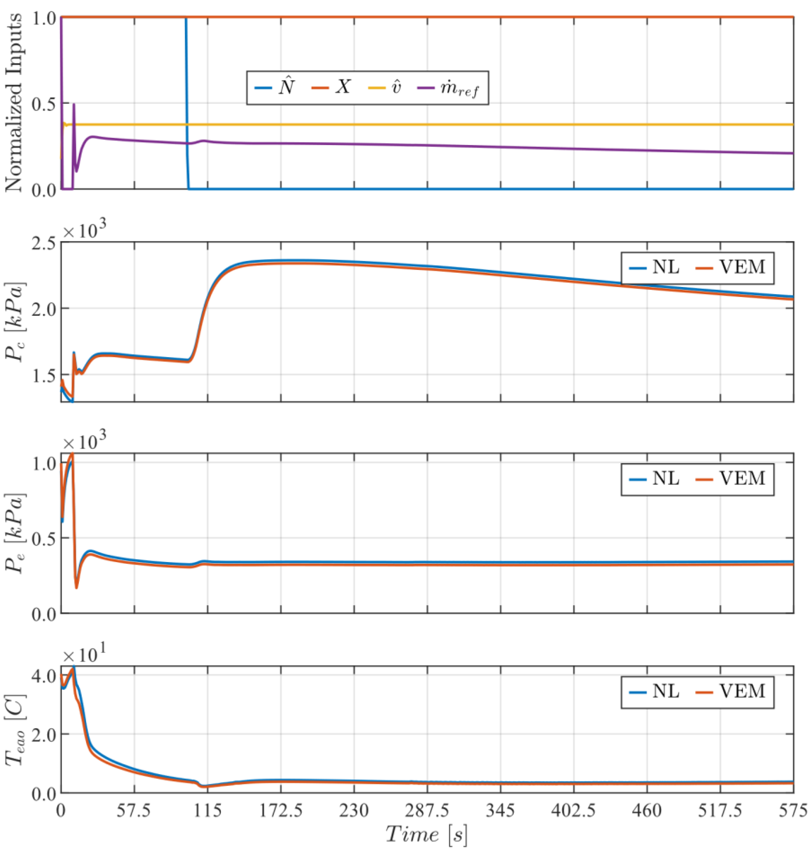
The mathematical models outlined in Section 2 were all implemented in Simulink to assess the performance of the A/C system. The calibration data came from VEM model data for the SC03 drive cycle, a standard drive cycle used by the Environmental Protection Agency (EPA) to assess vehicle fuel economy [18]. To be clear, the NL model implemented in Simulink is not able to be simulated as a standalone model. In order to simulate the NL model, time-series profiles for the controlled inputs () and external (uncontrolled) inputs () must be provided to the NL model, since the NL model does not compute these on its own. Recall that the model has been implemented in this way due to its intended usage as a model of the vehicle A/C system within a control framework, where it will accept external signals from the VEM model: the aim of the paper is to develop an improved NL model which more accurately captures the plant dynamics. The comparison between the nonlinear and VEM models for the SC03 cycle is shown in Figure 3. The comparison shown in Figure 3 demonstrates that the NL model is a good approximation of the behavior of the high-fidelity VEM model designed by the industrial partner, which is treated as the benchmark system in this case. For neatness, the vehicle speed input has been presented in a normalized form:
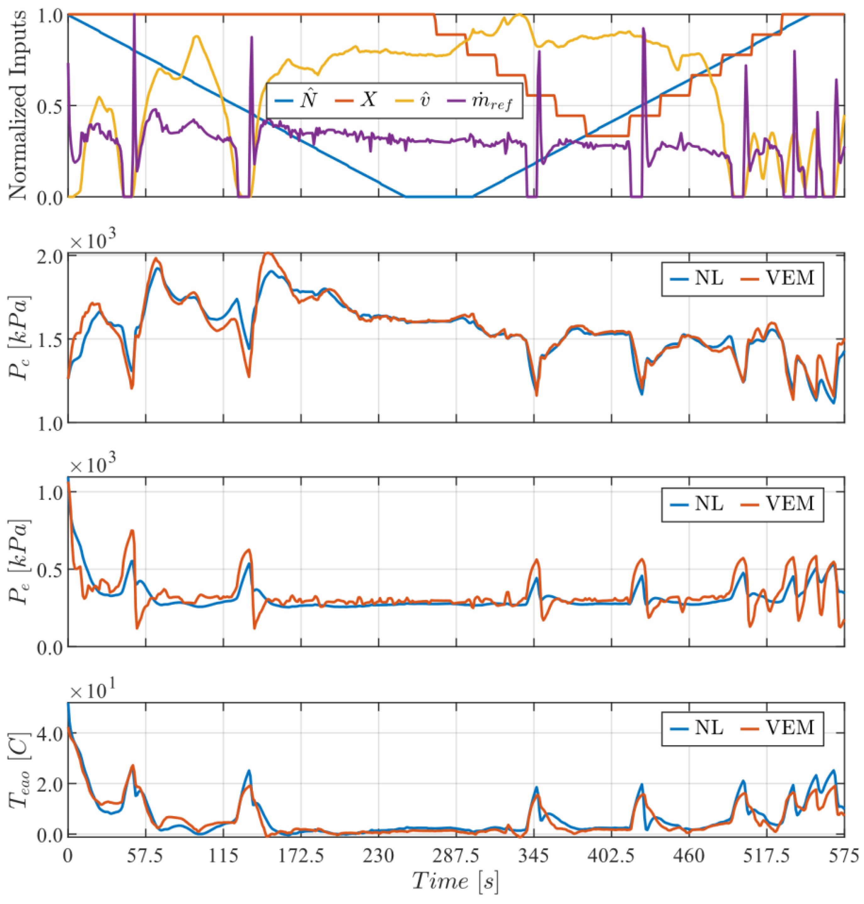
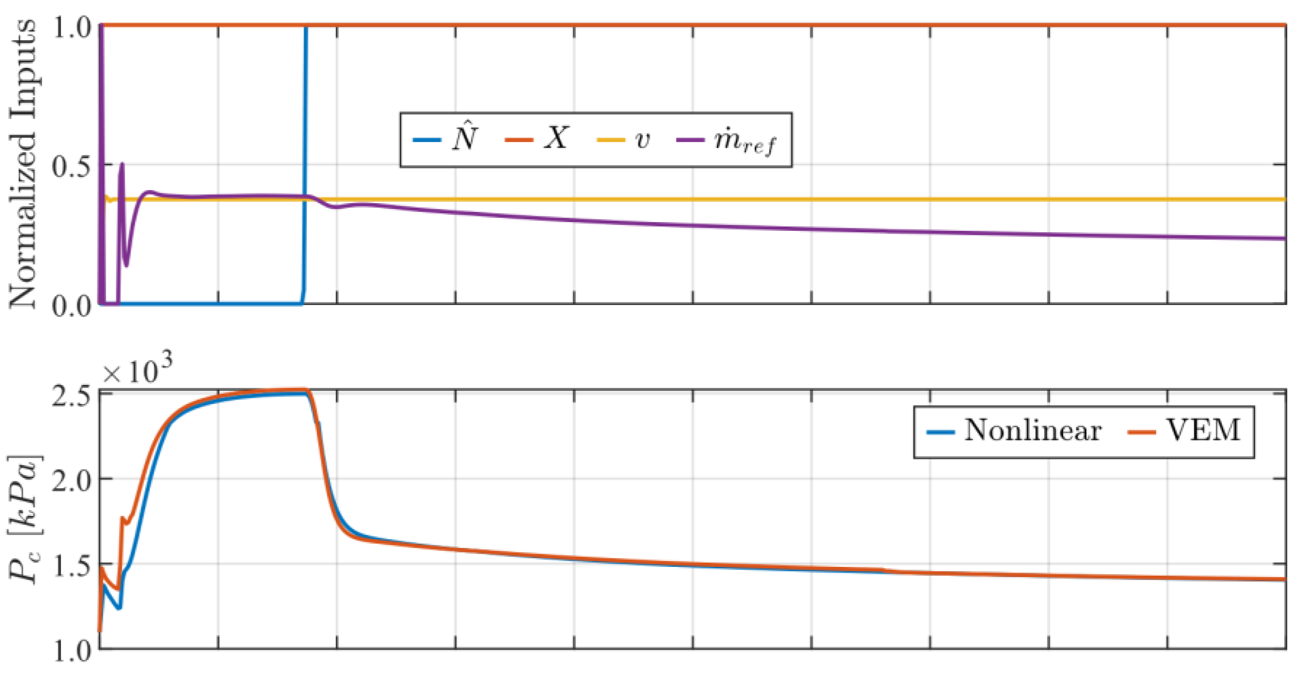
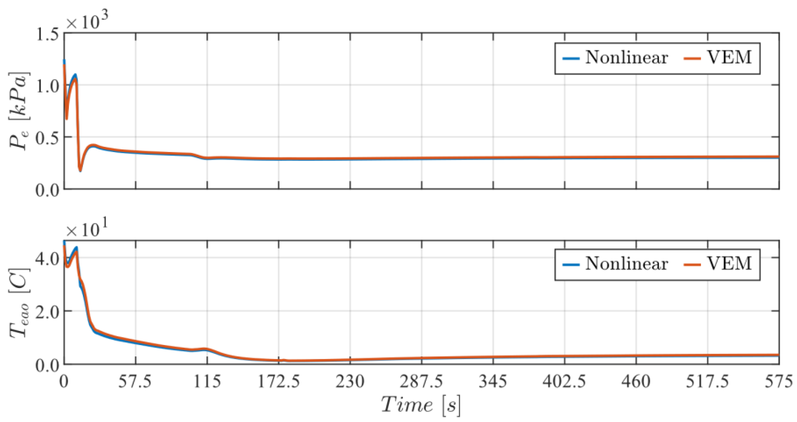
The normalized RMSE between the VEM and NL model signals shown in Figure 3 are displayed in Table 2. The error between the two models can be explained by approximations made in the NL model, such as curve fitting for the refrigerant thermal properties and underhood airflow. It can be seen that the evaporator pressure of the NL model has more inertia when comparing the transient portions of the response. The stiffness of the evaporator pressure of the NL model can be attributed to the multiplier, , introduced for the Nusselt number for the convective heat transfer. As the tuning parameter increases, the average agreement with the NL and VEM models improves, but the transient behavior becomes slower. For example, when the multiplier value is increased, the NL curve is shifted upward and compressed. Future research into this modeling can improve the response by investigating other methods to account for uncertainties with convective heat transfer modeling. To further assess the NL model, it was also run for a custom drive cycle to observe the agreement with the VEM model performance. For this custom drive cycle, the condenser fan and AGS actuator inputs were varied to induce transients in the model response. For the first half of the cycle, the AGS was held fully open while the fan speed ramped from max speed to zero, then back to max speed. For the second half of the cycle, the fan speed and AGS open-fraction were varied quasi-randomly to induce more transients in the model performance. The comparison between the NL model and the VEM model for this custom drive cycle is shown in Figure 4.
The normalized RMSE and maximum errors between the VEM and NL model signals shown in Figure 4 are displayed below in Table 2 and Table 3, respectively, demonstrating the NL model’s ability to handle transients arising from the inputs. It can be observed from Figure 3 and Figure 4 that the spikes in the refrigerant mass flow rate yield the greatest local error between the NL and VEM behaviors, causing the normalized RMSE to increase.
To further assess the model’s accuracy, the VEM and NL models were simulated using a constant vehicle speed profile of 13.4 m/s subject to an imposed fan speed step input from 2500 rpm to 0 rpm. For the entire cycle, the AGS was fully open, and the clutch was engaged. The results are shown in Figure 5. The same scenario was simulated using the opposite input step, where the fan speed was imposed from 0 rpm to 2500 rpm, shown in Figure 6. The ability of the NL model to correctly capture the settling time of the VEM model when subject to a step input from one of the controlled actuators, as well as the dynamics influenced by the refrigerant mass flow rate, is demonstrated. The RMSE and maximum errors for the results in Figure 5 and Figure 6 are shown in Table 4 and Table 5, respectively.
The errors associated with the drive cycle data are larger than those from the step responses since the transients are sharper in the drive cycles.
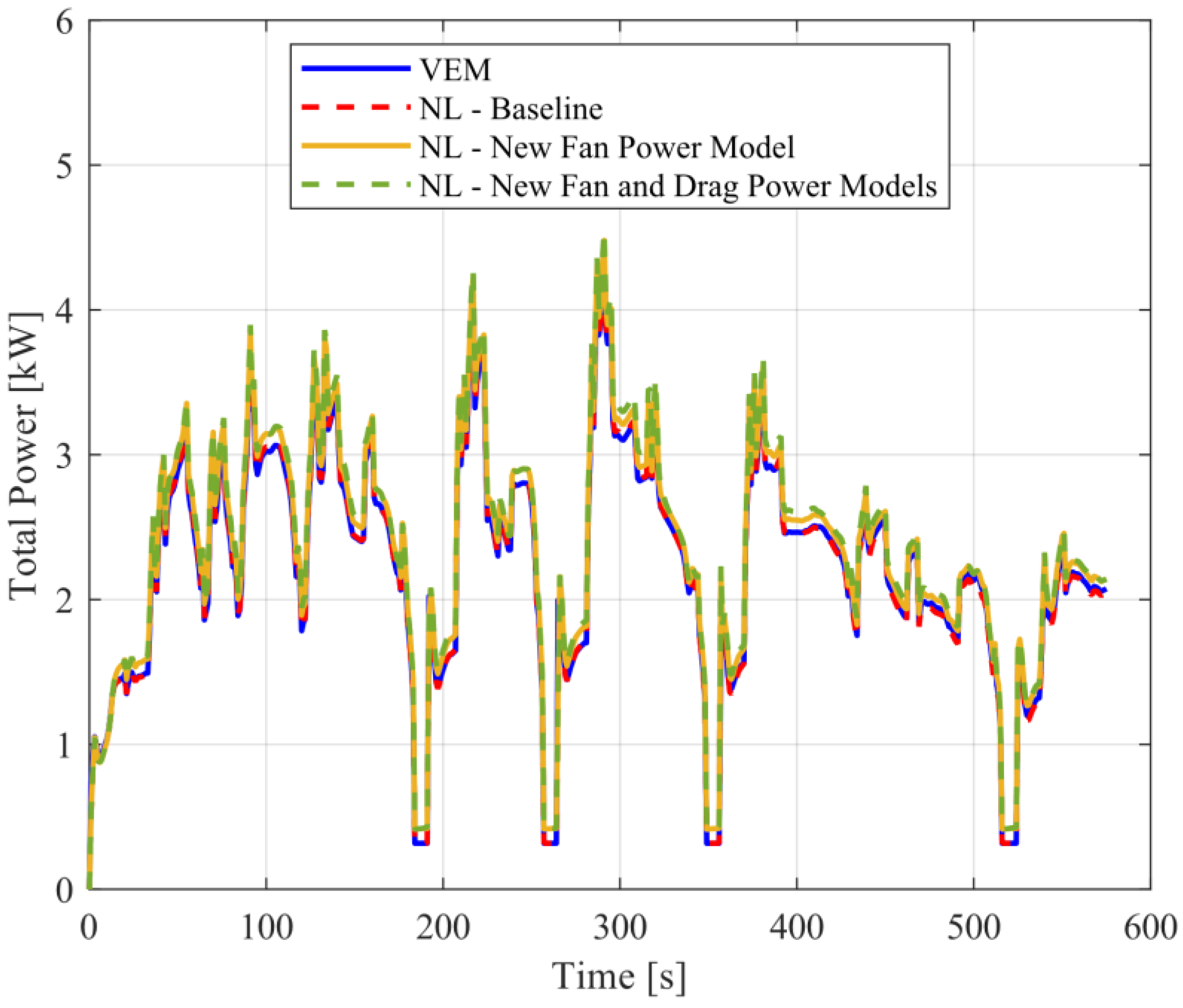
The power consumption of the A/C system was assessed for the same driving conditions used to obtain the results displayed in Figure 3. To show how the power consumption assessment of the A/C system has been developed through this work, three comparisons are made: the power consumption of the VEM model, which only measures the compressor and fan power; and the power consumption of the NL model using the same fan power model present in the VEM model, the power consumption of the NL model using Equation (11) for the fan power, and the power consumption of the NL model using Equations (11) and (14), including the additional drag power. These comparisons are shown in Figure 7.
From Figure 7, it can be seen that the VEM and NL—Baseline models have a good agreement for the total power consumed, which comes from the compressor and fan in these cases. When the new fan power model from Equation (11) is used instead of the VEM fan power model, there is a slight increase in the total power. One of the main takeaways from this figure is that the power consumption associated with additional aerodynamic underhood drag is minimal. This means that when additional cooling is required, opening the AGS will provide extra cooling at a small cost compared to other actuators, such as the fan and compressor.
The energy consumptions computed in each model are compared in Table 6. When the new fan power model in Equation (11) is added to the NL model, the total energy consumption is increased from 1284.2 kJ to 1336.6 kJ. This demonstrates that the baseline fan power model underpredicted the fan power consumption. The additional power consumed due to aerodynamic drag only slightly increases the total energy consumption computed, increasing it from 1336.6 kJ to 1353.2 kJ. Since the additional energy consumed due to the opening of the AGS is small, the addition of the AGS as a controllable actuator provides a valuable tradeoff to save energy elsewhere in the A/C system. When the AGS open-fraction increases, the flow entering the condenser increases, providing additional cooling to the system. When this happens, the compressor cooling effort can be reduced, saving on the energy usage of the compressor.
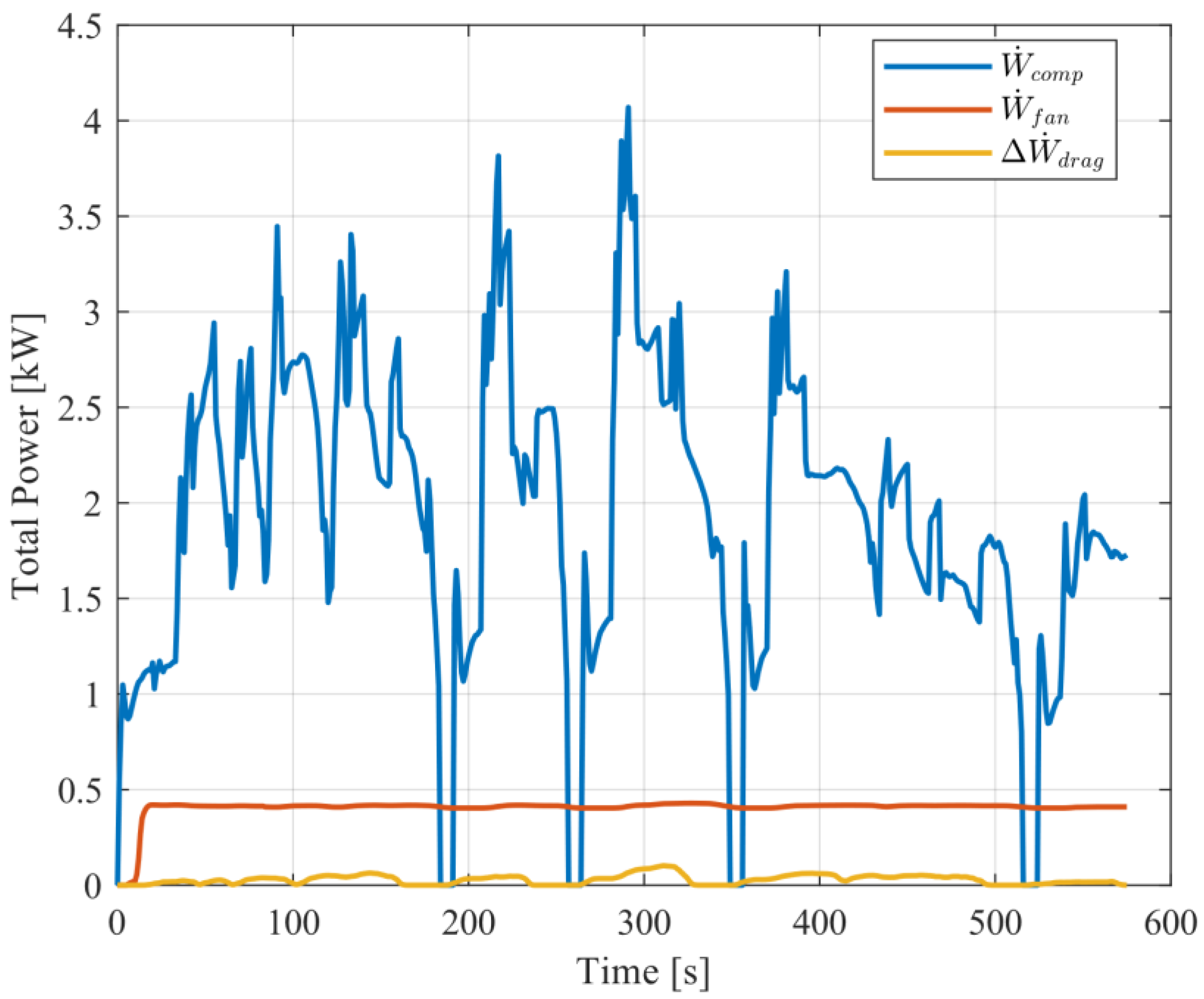
To gain insight into the individual contributions each component has on the total power consumption in the NL model, the compressor, condenser fan, and additional drag power are presented individually in Figure 8.
The compressor power consumption is driven by the mass flow rate of the refrigerant, which has a very strong impact on the compressor power, as can be seen. The impact of the volumetric airflow rate on the fan and additional drag power can also be seen. For the SC03 cycle shown in Figure 8, the fan speed and AGS positions are at their maximum physical values of 2500 rpm and fully open, respectively. Thus, any changes in the front-end airflow are caused by the vehicle speed, meaning the variations in the fan power and additional drag power observed in the figure are due to the change in vehicle speed.
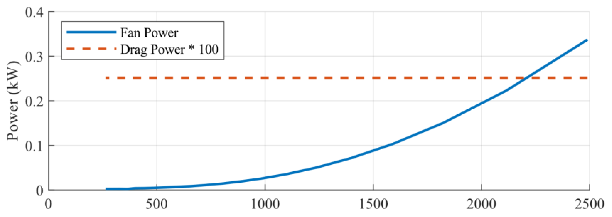
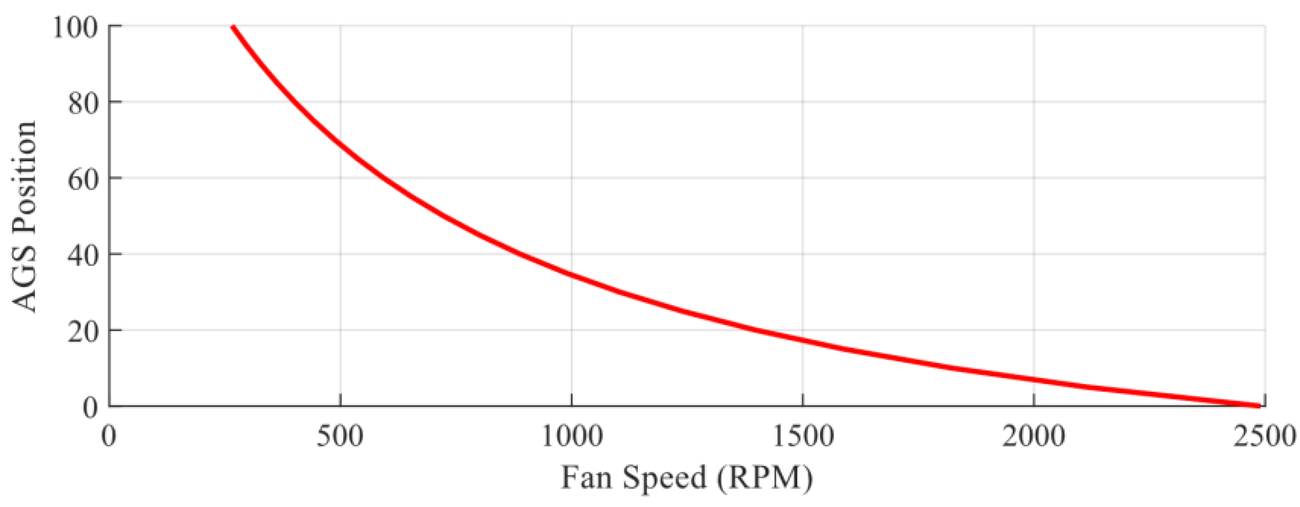
Figure 9 depicts the combinations of AGS position and fan speed inputs to maintain a constant underhood flow rate of 450 cfm and the power consumption associated with the fan and drag. In this driving condition, the power consumed by the fan is clearly much greater than the power consumed due to additional underhood drag. The same analysis was conducted for conditions where the drag power was more significant, specifically when the vehicle speed was much higher. The same findings were observed for these scenarios, where the fan power dominates the additional drag power. Figure 9 demonstrates that the same underhood airflow rate can be achieved using various combinations of AGS and fan inputs, but the power consumed is not constant. By opening the AGS, allowing more air to flow through the vehicle’s front end, the fan can reduce its rotational speed to achieve the same cooling flow but at reduced power consumption. This will be useful for control implementation where cooling performance and power consumption reduction are of interest.
4. Conclusions
In this paper, we have considered the AGS as a controllable actuator to regulate the underhood airflow and power consumption due to the underhood drag. The modeling work described in [11] was extended by developing a model for the airflow through the vehicle’s front end to allow the AGS actuation to be considered in the model. Models were created for the refrigerant thermodynamic properties, as well as the power consumption of the compressor, condenser fan, and underhood aerodynamic drag. The NL model was tuned to improve the agreement with various driving conditions, including the SC03 drive cycle and a custom drive cycle with strong transients in the controlled inputs. The NL model was validated against the behavior of a high-fidelity VEM model. The results showed that the overall performance of the system improved by reducing the error for the condenser pressure, evaporator pressure, and evaporator air temperature by 32.8%, 2.1%, and 2.6%, respectively. It was found that the power consumption associated with additional drag on the vehicle due to underhood airflow is a very small contribution to the overall power consumed by the A/C system, only 1.2% for the SC03 cycle. This means that considering the AGS as a controllable actuator can be useful in terms of reducing overall power consumption. By opening the AGS, additional cooling occurs due to the allowance of increased airflow through the vehicle’s front end, but only at a small power consumption cost. The cooling provided by the AGS airflow can reduce the cooling load on other actuators, such as the fan. The outcomes of this work will be used in a controller design in future work where the compressor clutch, fan rotational speed, and AGS open-fraction will be controlled to reduce the overall energy consumption of the A/C system.
Author Contributions
Conceptualization, T.P., J.J.D. and A.R.; methodology, T.P., J.J.D. and A.R.; software, T.P. and A.R.; validation, T.P. and J.J.D.; formal analysis, T.P.; investigation, T.P.; resources, J.J.D. and A.R.; data curation, T.P.; writing—original draft preparation, T.P.; writing—review and editing, J.J.D. and A.R.; visualization, T.P. and A.R.; supervision, J.J.D. and A.R.; project administration, J.J.D. and A.R.; funding acquisition, J.J.D. and A.R. All authors have read and agreed to the published version of the manuscript.
Funding
This research was funded by Mitacs Canada and Stellantis Canada, grant number IT25381 and The APC was funded by IT25381.
Data Availability Statement
Not applicable.
Acknowledgments
We thank Kevin Laboe, Nandan Sawkar, and Hamed Kharrati for supporting this work by providing insight, experimental data, and guidance.
Conflicts of Interest
The authors declare no conflict of interest.
Appendix A

Table A1.
System property values and units.
| System Model Property | Numeric Value | Units |
|---|---|---|
| 1.005 | ||
| 1.204 | ||
| 0.00018 | ||
| 1.505 | ||
| 0.910 | ||
| 3.022 | ||
| 0.898 | ||
| 0.974 | ||
| 0.1 | ||
| 0.0971 | ||
| 2.592 | ||
| 1.005 |
References
- Liu, J.; Zhou, H.; Zhou, X.; Cao, Y.; Zhao, H. Automative air conditioning system control—A survey. In Proceedings of the 2011 International Conference on Electronic Mechanical Engineering and Information Technology, Harbin, China, 12–14 August 2011; Volume 7, pp. 3408–3412. [Google Scholar]
- Jabardo, J.M.S.; Mamani, W.G.; Ianella, M.R. Modeling and experimental evaluation of an automotive air conditioning system with a variable capacity compressor. Int. J. Refrig. 2002, 25, 1157–1172. [Google Scholar] [CrossRef]
- Tian, C.; Li, X. Numerical simulation on performance band of automotive air conditioning system with a variable displacement compressor. Energy Convers. Manag. 2005, 46, 2718–2738. [Google Scholar] [CrossRef]
- El-Sharkawy, A.E.; Kamrad, J.C.; Lounsberry, T.H.; Baker, G.L.; Rahman, S.S. Evaluation of Impact of Active Grille Shutter on Vehicle Thermal Management. SAE Int. J. Mater. Manuf. 2011, 4, 1244–1254. [Google Scholar] [CrossRef]
- Shigarkanthi, V.; Damodaran, V.; Soundararaju, D.; Kanniah, K. Application of Design of Experiments and Physics based Approach in the Development of Aero Shutter Control Algorithm; SAE International: Warrendale, PA, USA, 2011. [Google Scholar] [CrossRef]
- Li, J.; Deng, Y.; Wang, Y.; Su, C.; Liu, X. CFD-Based research on control strategy of the opening of Active Grille Shutter on automobile. Case Stud. Therm. Eng. 2018, 12, 390–395. [Google Scholar] [CrossRef]
- Tandon, R.; Agrewale, M.R.; Vora, K. Aerodynamic Analysis of a Passenger Car to Reduce Drag Using Active Grill Shutter and Active Air Dam; SAE International: Warrendale, PA, USA, 2019. [Google Scholar] [CrossRef]
- Huang, Y.; Khajepour, A.; Khazraee, M.; Bahrami, M. A Comparative Study of the Energy-Saving Controllers for Automotive Air-Conditioning/Refrigeration Systems. J. Dyn. Syst. Meas. Control. 2016, 139, 014504. [Google Scholar] [CrossRef]
- Høgh, G.; Nielsen, R. Model based Nonlinear Control of Refrigeration Systems. Master’s Thesis, Aalborg Universitet, Copenhagen, Denmark, 2008; p. 115. [Google Scholar]
- Koo, B.; Yoo, Y.; Won, S. Super-twisting algorithm-based sliding mode controller for a refrigeration system. In Proceedings of the 2012 12th International Conference on Control, Automation and Systems, Guangzhou, China, 5–7 December 2012; pp. 34–38. [Google Scholar]
- Zhang, Q. “Modeling, Energy Optimization and Control of Vapor Compression Refrigeration Systems for Automotive Applications,” The Ohio State University. 2014. Available online: https://etd.ohiolink.edu/apexprod/rws_olink/r/1501/10?clear=10&p10_accession_num=osu1406121484 (accessed on 24 April 2022).
- Gamma, G. Technologies, “GT-SUITE,” GT-Suite Integrated Multi-Physics Systems Simulation. 2016. Available online: https://www.gtisoft.com/gt-suite/ (accessed on 23 November 2022).
- Zhong, Y.; Tiwari, A.; Jain, A.; Spasov, M. A Model of Heat Exchangers and Automotive AC System with Refrigerant-Oil Mixtures. In Proceedings of the International Refrigeration and Air Conditioning Conference, West Lafayette, IN, USA, 24–28 May 2021. [Google Scholar]
- Millo, F.; Rolando, L.; Graziano, E. Modelling of a BEV Thermal Management System and Development of Its Control Strategy in GT-SUITE; Politecnico di Torino: Torino, Italy, 2022. [Google Scholar]
- Çengel, Y.A.; Boles, M. Thermodynamics: An Engineering Approach, 9th ed.; McGraw-Hill Higher Education: Boston, MA, USA, 2019. [Google Scholar]
- Boyd, J.P. Six strategies for defeating the Runge Phenomenon in Gaussian radial basis functions on a finite interval. Comput. Math. Appl. 2010, 60, 3108–3122. [Google Scholar] [CrossRef]
- Dixon, S.L.; Hall, C.A. Fluid Mechanics and Thermodynamics of Turbomachinery, 7th ed.; Elsevier: Amsterdam, The Netherlands; Butterworth-Heinemann: Boston, MA, USA, 2014; ISBN 978-0-12-415954-9. [Google Scholar]
- Chengguo, L.; Brewer, E.; Pham, L.; Jung, H. Reducing Mobile Air Conditioner (MAC) Power Consumption Using Active Cabin-Air-Recirculation in A Plug-In Hybrid Electric Vehicle (PHEV). World Electr. Veh. J. 2018, 9, 51. [Google Scholar] [CrossRef] [Green Version]
Figure 1.
A/C system diagram.

Figure 2.
Pressure rise coefficient and normalized fan efficiency data with polynomial fits.

Figure 3.
VEM and NL pressure and temperature comparison for SC03 cycle.

Figure 4.
VEM and NL pressure and temperature comparison for custom drive cycle.

Figure 5.
VEM and NL model comparison for fan speed step input—2500 rpm to 0 rpm.

Figure 6.
VEM and NL model comparison for fan speed step input—0 rpm to 2500 rpm.


Figure 7.
Total power consumption comparison for the SC03 drive cycle.

Figure 8.
Compressor, condenser fan, and drag power consumption of NL model for SC03 cycle.

Figure 9.
AGS position, fan speed, and power for 450 cfm airflow at 13.4 m/s vehicle speed.


Table 1.
Model summary and comparison.
| Model Name | VEM | NL |
|---|---|---|
| Brief Model Description | High-fidelity vehicle dynamics model created using Gamma Technologies (GT) Suite [12] representing the real physical vehicle. | Nonlinear model implemented in Simulink based on Equations (2) and (4). |
| Pros | Holistic model of the entire vehicle, including all subsystems such as powertrain, A/C, cabin, electrical, etc. | Can accurately capture trends. |
| Cons | High computational cost and slow runtime due to model complexity. | Unable to run as a standalone model since it requires inputs in the form of time-series data from VEM model output. |
Table 2.
Normalized RMSE between VEM and NL models for SC03 and custom cycles.
| Parameter | |||
|---|---|---|---|
| SC03 Cycle Normalized RMSE | 4.4% | 7.2% | 3.8% |
| Custom Cycle Normalized RMSE | 6.5% | 7.8% | 4.6% |
Table 3.
Maximum error between VEM and NL models for SC03 and custom cycles.
| Parameter | |||
|---|---|---|---|
| SC03 Cycle Maximum Error | 354.3 | 209.8 | 5.3 |
| Custom Cycle Maximum Error | 205.9 | 286.5 | 10.3 |
Table 4.
RMSE between VEM and NL models for fan step input simulations.
| Parameter | |||
|---|---|---|---|
| RMSE for Negative Fan Step Input | 1.4% | 1.3% | 2.2% |
| RMSE for Positive Fan Step Input | 3.1% | 1.0% | 1.1% |
Table 5.
Maximum error between VEM and NL models for fan step input simulations.
| Parameter | |||
|---|---|---|---|
| Max Error for Negative Fan Step Input | 43.7 | 53.0 | 5.6 |
| Max Error for Positive Fan Step Input | 370.1 | 47.9 | 2.5 |
Table 6.
Energy consumption comparison for SC03 cycle.
| Model Name | VEM | NL—Baseline | NL—New Fan Power Model | NL—New Fan and Drag Power Models |
|---|---|---|---|---|
| Compressor Energy [kJ] | (86.1%) | (86.1%) | (82.7%) | (81.7%) |
| Fan Energy [kJ] | 179 (13.9%) | 179 (13.9%) | 231 (17.3%) | 231 (17.1%) |
| Drag Energy [kJ] | N/A | N/A | N/A | 16.7 (1.2%) |
| Total Energy [kJ] | ||||
| Percentage Change [%] | N/A | −0.200 | 3.87 | 5.16 |
Disclaimer/Publisher’s Note: The statements, opinions and data contained in all publications are solely those of the individual author(s) and contributor(s) and not of MDPI and/or the editor(s). MDPI and/or the editor(s) disclaim responsibility for any injury to people or property resulting from any ideas, methods, instructions or products referred to in the content. |
© 2023 by the authors. Licensee MDPI, Basel, Switzerland. This article is an open access article distributed under the terms and conditions of the Creative Commons Attribution (CC BY) license (https://creativecommons.org/licenses/by/4.0/).
Share and Cite
MDPI and ACS Style
Parent, T.; Defoe, J.J.; Rahimi, A. Nonlinear Modeling of an Automotive Air Conditioning System Considering Active Grille Shutters. Modelling 2023, 4, 70-86. https://doi.org/10.3390/modelling4010006
AMA Style
Parent T, Defoe JJ, Rahimi A. Nonlinear Modeling of an Automotive Air Conditioning System Considering Active Grille Shutters. Modelling. 2023; 4(1):70-86. https://doi.org/10.3390/modelling4010006
Chicago/Turabian StyleParent, Trevor, Jeffrey J. Defoe, and Afshin Rahimi. 2023. "Nonlinear Modeling of an Automotive Air Conditioning System Considering Active Grille Shutters" Modelling 4, no. 1: 70-86. https://doi.org/10.3390/modelling4010006