Off-Design Analysis Method for Compressor Fouling Fault Diagnosis of Helicopter Turboshaft Engine

Abstract

Fouling, caused by the adhesion of fine materials to the blades of the compressor’s last stages, changes the airfoil’s shape and function and the inlet flow angle on the blades. As the fouling increases, the range of influence increases, and the mass flow rate and overall engine efficiency reduce. Therefore, the compressor is choked at lower speeds. This study aims to simulate compressor performance during off-design conditions due to fouling and to present an approach for modeling faults in diagnostic and health monitoring systems. A computational fluid dynamics analysis is carried out to evaluate the proposed method on General Electric’s T700-GE turboshaft engine, and the performance is evaluated at different flight conditions. The results show promising outcomes with an average accuracy of 88% that would help future turboshaft health monitoring systems.

1. Introduction

When helicopters fly in harsh environments such as cities, deserts, or saltwater seas, pollution, sand, salt, and moisture are among the destructive factors that the engine faces. Fouling in compressors is one of the most common problems caused by these natural and environmental factors. The consequences of fouling can severely affect the performance of turboshaft engines.

Fouling, formed on the compressor blades, changes the airflow trajectories and reduces the surge range [1]. This additionally increases the compressor’s sensitivity to instabilities. Therefore, the airflow reaches a choked condition at lower speeds, generally measured in revolutions per minute (RPMs) [2]. With the growth and continuation of fouling, the mass flow rate (MFR) is more affected and causes a sharp drop in the compressor pressure ratio (CPR), reducing the output power and increasing the specific fuel consumption (SFC). Therefore, it is one of the essential factors in off-design performance and will determine the performance range for the engine health monitoring (EHM) system [3].

With the advent of the new generation of variable-speed engines and efforts to increase power and reduce fuel consumption and emissions, design requirements lead engineers to a higher-pressure ratio and more accurate control systems in the compressor. Therefore, it is necessary to develop diagnostic systems to synthesize the engine’s off-design performance and quickly identify fouling in the compressor from other factors that can create similar conditions.

In gas turbine fault diagnostics, engine manufacturers have devised several methods over the past four decades [4,5].

Table 1. Fault diagnostic methods for turboshaft engines.

Author	Ref.	Year	Classification
Saravanamuttoo, et al.	[6]	1989	Computer Simulation Techniques
Dash, et al.	[7]	2000	MB and Data-driven
Yang, H., et al.	[8]	2014	MB, and local optimization
Zhao, et al.	[3]	2016	MB, DD, and Knowledge-based
Zeng, et al.	[9]	2018	MB, and direct problem
Vulpio, A., et al.	[10]	2021	MB, and Hybrid
Suman, et al.	[1]	2021	MB, and particle impact influence

lists some of the fault diagnostic methods for turboshaft engines. The ability to use data analysis in engines and proactively monitor fouling progression is paramount. Thus, Saravanamuttoo et al. [6] conducted extensive and fundamental research on the performance of clean and fouled compressors in various types, levels, and locations of known faults. These studies led to the modeling and sensitivity analysis of parameters affecting fouling.

The model-based (MB) methods are the first category of gas turbine diagnostic methods that rely on the engine’s thermodynamic model. The second category is the data-driven (DD) approach, with a different diagnostic approach that uses maintenance processes and historical data to devise decisions [7].

In some studies, the stage-stacking method has been used due to high speed and a good adaptation of local optimization models to field data [8]. The overall effect of the one-stage fouling simulation is considered to calculate the full compressor performance. So, this method is not based on detailed analysis.

Zhao et al. [3] have developed a physics-based adaptive model to evaluate performance deltas and correct the data to reference conditions. At the same time, a DD correlation algorithm identifies the most likely matches within a fault signatures database.

Zeng et al. [9,11] developed modeling for the impacts of fouling on the overall engine performance, and N. Casari et al. [12] developed a multistage compressor performance simulation model based on one-dimensional analysis. These simulations are used when fouling is present, and fault characteristics are known.

Recently, hybrid models have enhanced these weaknesses and have received more attention as they improve the accuracy and speed of data analysis [10,13,14]. In [10], a turboshaft engine’s multistage axial-flow compressor is employed to study the fouling rate on rotor blades and stator vanes from both numerical and experimental standpoints.

In 2021, Suman et al. [1] published significant research on modeling based on particle impact influence and trajectories. These models are very accurate but are complicated, slow, and time-consuming for diagnostic systems in multistage axial flow compressors.

This proposed research aims to develop a novel MB method for the EHM system of turboshaft engines that require fewer data/parameters to work while maintaining or improving the detection and isolation schemes’ accuracy.

2. Problem Definition

Reviewing the literature, two main issues emerge from the analysis of these engines under harsh conditions related to fouling:

Lack of engine data: The development of fault diagnostic methods requires relevant and reliable data to sufficiently represent healthy and unhealthy engine conditions. It is difficult to obtain the required data because of the limited availability of gas turbine operational data and a lack of deteriorated engine data. Thus, most of the significant studies in the past are based on the analysis of industrial or axial compressors [15]. Considering the use of both axial and centrifugal compressors in helicopter turboshaft engines, this study can complement previous studies.

Engine’s speed and flight conditions: The new turboshaft engines [16] experience additional issues with the variability of the engine’s speed, such as instability in compressor operations, vibrations and resonance, and control of flow through inlet guide valves, among others. Another factor presented in this research is the use of variable speed engines, sensitivity analysis, and fouling reactions to the cycle in different flight conditions.

The objective of this paper is to address the abovementioned issues under the formal problem definition below;

1. Creating an accurate dataset: The aero-thermodynamic model, protection design guidelines (PDG), and subsystem data (SSD) will be combined and presented on the dataset. For fault diagnosis and isolation (FDI) system adaptation with the aero-thermodynamic model, technology coefficients will be applied to all parameters and effective components in the diagnostic modeling process [16]. If the International Civil Aviation Organization (ICAO) or the manufacturer issue recalls, repairs, and overhaul (MTO) documentation, the FDI system must be updated to account for these updated guidelines. Therefore, using coefficients allows us to define the accuracy and sensitivity of detection in the engine’s components.

Flight conditions including temperature ($T_0$), pressure ($P_0$), Mach ($M_0$), power requested by the pilot (${\mathsf{{\rm P}}}_{operator}$), power produced by the engine (${\mathsf{{\rm P}}}_e$), number of revolutions per minute of the gas turbine ($N_{GGT}$) and free turbine ($N_{FPT}$), compressor pressure ratio (${\pi }_c$), turbine gas temperature (TGT), engine outlet temperature (EGT), fuel mass flow rate (${\dot{m}}_f$), bleed mass flow rate (${\dot{m}}_{\beta }$) and cooling (${\dot{m}}_{\epsilon }$), the angle of the inlet guide (${\alpha }_{IGV}$), and the engine control unit (ECU) data inspected by the PDG are all parameters used in the FDI system. Figure 1 presents the parameters of the aerothermodynamic model and the importance of effective coefficients in the process of the FDI.

2. Tracking an off-design condition: Any defect or change in a component’s performance will generate an off-design dataset. The compressor’s map and turbine gas temperature (TGT) are essential data for flow status [17] and fouling identification. Therefore, flow control is a key factor for fouling studies.

3. Identifying faults in the system: Fouling detection is an essential step in fault diagnostics. Trend shift detection and binary decision approaches are commonly applied techniques [18]. This study is performed based on the difference between the off-design and on-design datasets, and the relationship between them is highly nonlinear. The diagnostics problem’s nonlinear complexity increases as two or more components are affected simultaneously, and component faults coexist. Thus, the diagnostic system to be proposed should be capable of dealing with engine behavior’s nonlinear nature [19].

3. Methodology

Figure 2 shows the reference stations for the inlet, compressor, burner, nozzle guide vane (NGV), gas generation turbine (GGT), free power turbine (FPT), nozzle, and engine reduction gearbox (ERG) in a helicopter turboshaft engine. This section outlines the off-design analysis modeling for the compressor fouling diagnostics process between stations 2 and 3 to solve the problem where the engine performance is known (MFR, CPR, SFC, efficiency, etc.) and the fault severity, type, and location must be determined.

In engine design, a dataset is considered the primary reference point. Changing the input data will yield secondary datasets (on-design) at each flight condition. By making any changes in one of the parameters, other parameters will also change, and the system will enter off-design conditions. Therefore, the system’s off-design output can be compared with its on-design at any given time to generate residuals and identify faulty behavior and its characteristics.

The compressor fouling modeling is considered for the off-design system at three levels. These three levels are (i) low with 1%, (ii) medium with 2%, and (iii) high with 3%, air MFR decrease in the compressor. In order to model power, efficiency, and other performance parameters, new calculations are performed at each stage as a function of the corrected MFR. Figure 3 illustrates the model’s relationships between independent and dependent variables and the overall process flow.

The proposed modeling is structured in six steps as follows. The first step is to calculate the engine output power.

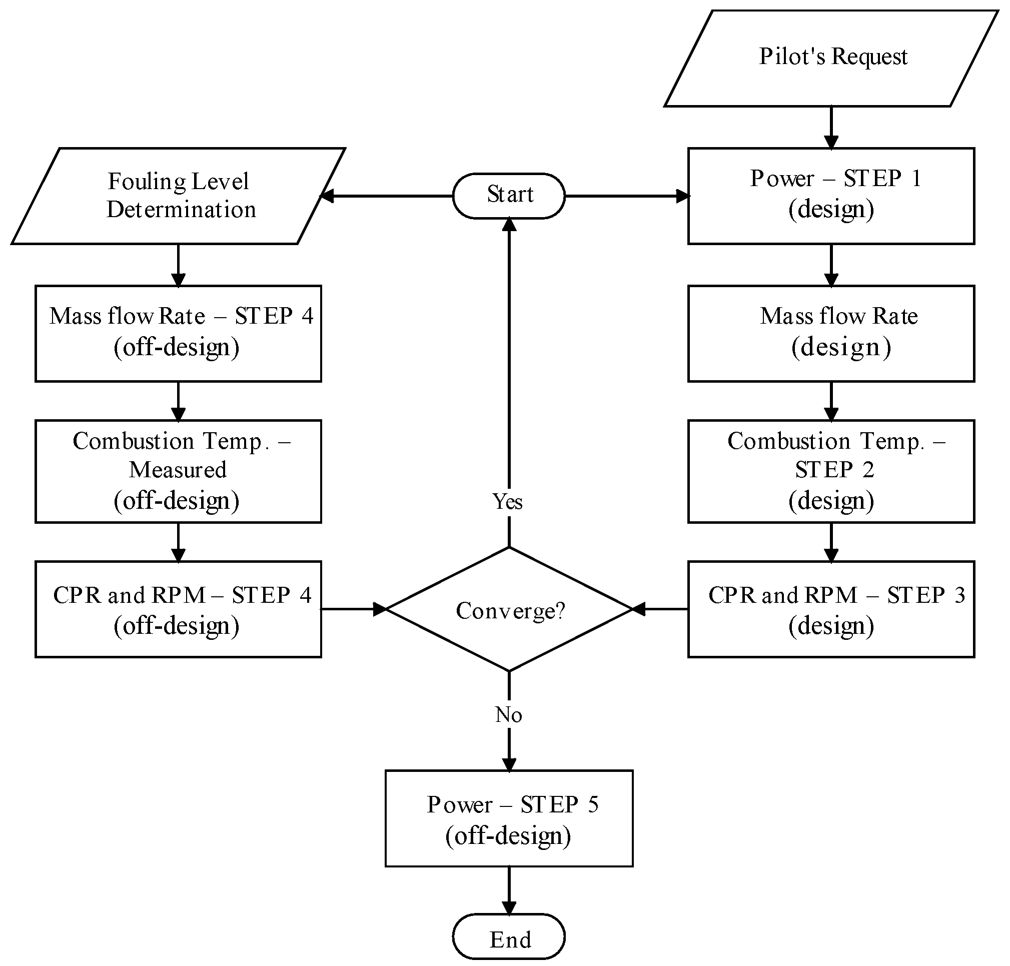
3.1. Engine Cycle—Power (Step 1)

The parameter that determines the instantaneous data values in the on-design condition is the engine power (${\mathrm{P}}_e$). Engine power is calculated from Equation (1) based on the rotors’ condition, flight condition, and subsystems requirements [20].

$${\mathsf{{\rm P}}}_e=\frac{{\mathsf{{\rm P}}}_{mr}+{\mathsf{{\rm P}}}_{tr}+{\mathsf{{\rm P}}}_{accs}}{n_e {\eta }_g{\eta }_m\left(\frac{P_0}{P_{0R}}\sqrt{\frac{T_0}{T_{0R}}}\right)}$$

(1)

where $n_e$ is the number of active engines. Moreover, mechanical efficiency (${\eta }_m$) and gearbox transmission efficiency (${\eta }_{gt}$) denotes the level of technology used in manufacturing. The power used in the main rotor (${\mathsf{{\rm P}}}_{mr}$), the tail rotor (${\mathsf{{\rm P}}}_{tr}$), and accessories (${\mathsf{{\rm P}}}_{accs}$) are proportional to the total power produced by the engine. Finally, $\frac{P_0}{P_{0R}}\sqrt{\frac{T_0}{T_{0R}}}$ is the ambient term. $P_0$ and $T_0$ are pressure and temperature at station 0. Subscript “$R$” refers to the reference data.

3.2. Engine Cycle—Combustion Temperature (Step 2)

After determining the power, the next step is calculating the energy in the combustion chamber. Since fuel has a specific heat value ($h_{PR}$), under normal conditions, the amount of energy will be directly related to temperature. Therefore, the calculation of combustion temperature ($T_4$) as one of the most critical operating/control parameters to obtain the required power can be obtained from Equation (2) [16].

$$T_4=\frac{1}{C_{P3}{C}_{P4}{T}_0}{\left[\frac{h_{PR}{\eta }_{cc}{\mathsf{\tau }}_d}{\frac{{\dot{m}}_{3.1}\left(1-{\mathsf{\tau }}_d\right)}{SFC.{\mathrm{P}}_{\mathrm{e}}}+1}\right]}^2$$

(2)

where ${\eta }_{cc}$ is combustion chamber efficiency and denotes the impact coefficient of the technology used. ${\mathsf{\tau }}_d$ is the total temperature ratio caused only by wall friction effects, and $C_P$ is the specific heat at constant pressure. ${\dot{m}}_{3.1}$ gives the output air mass flow rate from the compressor.

The combustion temperature difference causes rotation of the shaft and defines the compressor’s operating conditions as detailed in Step 3.3.

3.3. Engine Cycle—Compressor (Step 3)

The energy released on the turbine blades causes the compressor to rotate and the CPR. The CPR for the engines used to date is between 1:6 and 1:22, and polytropic efficiency ($e_c$) is a function of the technology level used (

Table 2. Compressor polytropic efficiency levels. Data taken from Ref. [16]. Copyright 2023 SAE International.

	Level of Technology
Factor	1	2	3	4
$e_c$	0.80	0.84	0.88	0.90

) in the compressor stages.

The compressor’s temperature ratio (${\tau }_c$), pressure ratio (${\pi }_c$), and efficiency (${\eta }_c$) can be obtained from Equation (3) [21].

$$\begin{gathered} {\tau }_c=\frac{1}{{\tau }_i}\sqrt{\frac{C_{P4}{T}_4}{C_{P3}{T}_0}} \\ {\pi }_c={\left({\tau }_c\right)}^{\frac{{\gamma }_c{e}_c}{{\gamma }_c-1}} \\ {\eta }_c=\frac{{\pi }_c{}^{\frac{{\gamma }_c-1}{{\gamma }_c}}-1}{{\tau }_c-1} \end{gathered}$$

(3)

where $\gamma$ is the heat capacity ratio, and ${\tau }_i$ is the temperature ratio of the engine inlet.

The gas carries the energy released in the combustion chamber and sits on the turbine blades, causing the gas generator turbine (GGT) to rotate. The turbine speed changes outside the reference design point and can be obtained from Equation (4) [22]. Subscript “$R$” refers to the reference.

$$N_{GGT}=N_{GGT-R}\sqrt{\frac{T_0{\tau }_i\left({\tau }_c-1\right)}{{\left|T_0{\tau }_i\left({\tau }_c-1\right)\right|}_R}}$$

(4)

The data set at the design point is completed, and the parallel off-design analysis will be examined in the next step.

3.4. Fouling Effect—Compressor (Step 4)

The cross-section of the fluid flow in the compressor decreases as the fouling progresses on the compressor blades, reducing the mass flow rate. The MFR under fouling conditions is obtained from Equation (5). Subscript “F” refers to the fouling and for further details on the derivation, see Appendix A.1.

$${\dot{m}}_{2.2F}={\dot{m}}_{2.2}\frac{\sqrt{T_4}}{P_2{\pi }_c}\left(\frac{P_{2F}{\pi }_{cF}}{\sqrt{T_{4F}}}\right)$$

(5)

where $P_2$ is the total pressure at station 2, where the engines have a pressure sensor.

Small MFR changes will cause drastic changes in the pressure ratio based on the compressor’s sensitivity to MFR changes. The compressor pressure ratio under the fouling (${\pi }_{cF}$) condition is formulated in Equation (6). Details on the derivation of this equation are represented in Appendix A.2.

$${\pi }_{cF}={\left[1+\left(\frac{T_2}{T_4}\right)\left(\frac{T_{4F}}{T_{2F}}\right)\left({\pi }_c^{\frac{{\gamma }_c-1}{{\gamma }_c{e}_c}}-1\right)\right]}^{\frac{{\gamma }_c{e}_c}{{\gamma }_c-1}}$$

(6)

The combustion chamber’s flame temperature and chemical reactions are affected by reducing the pressure ratio of the incoming airflow from the compressor. Although the sprayed fuel is constant, these changes show their impact by reducing the turbine blades’ discharged energy and the shaft’s rotational speed. Changes in the compressor rotational speed under fouling conditions can be obtained from Equation (7).

$$N_{GGT-F}=N_{GGT}\sqrt{\frac{{\pi }_{cF}^{\frac{{\gamma }_c-1}{{\gamma }_c{e}_c}}-1}{{\pi }_c^{\frac{{\gamma }_c-1}{{\gamma }_c{e}_c}}-1}}$$

(7)

Constraining the flow passage at the end of the compressor increases the air mass density, increasing the pressure and temperature at the compressor inlet. Assuming that the position of the inlet guide vane blades (constant volume condition) does not change, Amontons’s law [23] will be used to calculate the inlet pressure ($P_{2F}$). Rearranging Equation (7) and using Amontons’s law, the compressor’s inlet temperature under fouling conditions can be obtained from Equation (8).

$$T_{2F}=T_2{\left[\frac{{\pi }_c}{{\dot{m}}_{2.2}\sqrt{T_4}}\left(\frac{{\dot{m}}_{2.2F}\sqrt{T_{4F}}}{{\pi }_{cF}}\right)\right]}^2$$

(8)

where $T_2$ is the total temperature at station 2, where the engines have a temperature sensor.

The next step will be to define the engine power at the fouling condition.

3.5. Fouling Effect—Power (Step 5)

To stabilize the flow through the compressor stages, at the end of the axial compressor, bleed valves/bands (β) reduce the relative air pressure and prevent stall/surge. On the other hand, fouling results in massive changes in the compressor’s mass flow rate, pressure ratio, and combustion chamber temperature, all of which will affect the performance of turboshaft engines, including its power output. The derivation process in Appendix A.3 calculates the power reduction with fouling progression from Equation (9).

$$\begin{array}{c}{\mathrm{P}}_{\mathrm{eF}}={\mathrm{P}}_{\mathrm{e}}\left(\frac{{\dot{m}}_{2.2F}}{{\dot{m}}_{2.2}}\right)\left(\frac{1+f_F-\beta }{1+f-\beta }\right)\left(\frac{T_{5F}}{T_5}\right)\left[\frac{1-{\left(\frac{P_0}{{\mathrm{P}}_{5F}}\right)}^{\frac{\left({\gamma }_t-1\right)e_t}{{\gamma }_t}}}{1-{\left(\frac{P_0}{{\mathrm{P}}_5}\right)}^{\frac{\left({\gamma }_t-1\right)e_t}{{\gamma }_t}}}\right]\hfill \\ T_{5F}=T_{4F}-\frac{C_{P3}{T}_{2F}\left[{\left({\pi }_{cF}\right)}^{\frac{{\gamma }_c-1}{{\gamma }_c{e}_c}}-1\right]}{C_{P4}{\eta }_m\left(1+f_F-\beta \right)}\hfill \\ P_{5F}=P_0{\pi }_i{\pi }_d{\pi }_{CC}\left[{\pi }_{CF}{\left(1-\frac{T_{4F}-T_{5F}}{{\eta }_{GGT}{\mathrm{T}}_{4F}}\right)}^{\frac{{\gamma }_t}{\left({\gamma }_t-1\right)e_t}}\right]\hfill \end{array}$$

(9)

where $T_5$ is the total temperature at station 5, where the engines have a temperature sensor. f is the fuel-to-air mass flow ratio, which can be calculated using the level of technology chosen for the design, the inlet and diffuser pressure ratio, the combustion chamber pressure ratio, and the polytropic efficiency of the compressor and turbine as detailed in [16]. In addition, the mechanical and turbine efficiency factors can be obtained from the manufacturers.

With power values at the off-design situation, specific fuel consumption and efficiency can be defined in step 6.

3.6. Fouling Effect—SFC and Efficiency (Step 6)

Since the fuel mass flow rate (${\dot{m}}_f$) is based on the requested power and the inlet air conditions of the engine, under the same conditions, the specific fuel consumption of turboshaft engines with fouling can be obtained from Equation (10).

$$SF{C}_F=\frac{{\dot{m}}_f}{{\mathrm{P}}_{\mathrm{eF}}}$$

(10)

Finally, using the fuel’s specific heat, the engine’s thermal efficiency under fouling conditions (${\eta }_{th-F}$) is calculated from Equation (11).

$${\eta }_{th-F}=\frac{{\mathrm{P}}_{\mathrm{eF}}}{{\dot{m}}_f{h}_{PR}}=\frac{1}{SF{C}_F h_{PR}}$$

(11)

In the following section, the proposed methodology results of a case study are presented and discussed in detail.

4. Results and Discussion

To verify the proposed process in the previous section, the T700-GE turboshaft engine on a Sikorsky UH-60A helicopter is presented as a case study in this section. The calculations presented here are based on

Table 3. T700-GE reference data in on-design condition. Data taken from Ref. [16]. Copyright 2023 SAE International.

Parameters		Value	Unit
Number of engines	$(n_e$)	2	-
Diffuser temp. ratio	$({\mathsf{\tau }}_d$)	0.399	-
Compressor inlet area	$(A_2$)	0.02543	[m2]
Air mass flow rate at the design point	$({\dot{m}}_{2.2}$)	4.6122	[kg/s]
Compressor pressure ratio at the design point	$({\pi }_c$)	17.5	-
Compressor polytropic efficiency	$(e_c$)	0.821	-
Compressor speed at the design point	$\left(N_{GGT-R}\right)$	44,700	[rpm]
Combustion chamber temperature at the design point	$({\mathrm{T}}_4$)	1124	[°K]
Combustion chamber efficiency	$({\eta }_{cc}$)	0.985	-
Fuel mass flow rate at the design point	$({\dot{m}}_f$)	0.1004	[kg/s]
Fuel upper heat of combustion	$(h_{PR}$)	43,100	[kJ/kg]
Specific fuel consumption at the design point	$(SFC$)	7.8569 × 10−8	[kg/J]
Free power turbine rotational speed at the design point	$\left(N_{FPT-R}\right)$	20,900	[rpm]
Free power turbine power at the design point	$({\mathsf{{\rm P}}}_e$)	1329.9	[kW]
Mechanical efficiency	$({\eta }_m$)	0.99	-
Gear transmission efficiency	$({\eta }_{gt}$)	0.95	-

, which lists the reference design data for this engine.

There are two configurations for turboshaft engine inlets (i) static and (ii) dynamic. The T700-GE is a mid-range engine that houses a dynamic-type inlet. Additionally, this engine uses axial and centrifugal compressors for power assurance during high-speed helicopter missions in harsh environments. The real dimensions are used in the simulation of the compressor. However, since the pressure distribution is more important in the analysis of the results, the actual numerical location of each pressure point is not as important to show in the following figures. Figure 4 shows the configuration and pressure distribution in T700-GE compressors.

Although Table 3 provides general information about the engine at an altitude of 500 m above sea level at the reference point, the sensitivity and reaction of the parameters to fouling in hover, forward/backward, climb/descent, and combined flight maneuvers at an altitude of 2572 m above sea level are modeled and presented in

Table 4. Fouling performance prediction on different flights for T700-GE.

Status	Engine Data
	${\mathit{M}}_0$	${\dot{\mathit{m}}}_{2.2}$	${\mathit{T}}_2$	${\mathit{P}}_2$	${\mathit{\pi }}_{\mathit{C}}$	${\mathit{T}}_4$	${\dot{\mathit{m}}}_{\mathit{f}}$	${\mathit{N}}_{\mathit{G}\mathit{G}\mathit{T}}$	${\mathit{N}}_{\mathit{F}\mathit{P}\mathit{T}}$	${\mathit{Q}}_{\mathit{F}\mathit{P}\mathit{T}}$	${\mathit{{\rm P}}}_{\mathit{e}}$	SFC	${\mathit{\eta }}_{\mathit{t}\mathit{h}}$
Hovering maneuver
On-Design [16]	0.119	2.746	112	89,424	14.72	1015	0.0524	47,947	23,023	289	667	7.8569	0.29
Off-Design (1%)		2.719	112	89,454	14.52	1008	0.0421	47,768	22,849	284	649	6.4942	0.36
Off-Design (2%)		2.691	112	89,469	1.019	5.070	0.0155	3342	FW *	000.00	000	-	0.00
Off-Design (3%)		2.664	112	89,501	1.019	5.177	0.0153	3342	FW *	000.00	000	-	0.00
Forward flight (minimum power)
On-Design [16]	0.192	2.280	112	90,850	8.17	755	0.0264	36,223	15,176	221	336	7.8569	0.29
Off-Design (1%)		2.257	112	90,850	8.05	748	0.0302	36,070	15,013	219	329	9.1747	0.25
Off-Design (2%)		2.234	112	90,921	1.048	12.96	0.0121	4713	FW *	000.00	000	-	0.01
Off-Design (3%)		2.212	112	90,906	1.049	13.24	0.0120	4761	FW *	000.00	000	-	0.00
Forward flight (maximum velocity)
On-Design [16]	0.563	5.2041	119	109,800	14.15	1118	0.1170	43,472	20,795	715	1489	7.8569	0.29
Off-Design (1%)		5.152	119	109,785	13.96	1110	0.0941	43,315	20,659	700	1449	6.4903	0.36
Off-Design (2%)		5.100	119	109,774	1.021	6.058	0.0350	3217	FW *	000.00	000	-	0.01
Off-Design (3%)		5.048	119	109,779	13.58	1094	0.0915	43,003	20,350	681	1387	6.5911	0.35
Climbing flight (maximum velocity)
On-Design [16]	0.242	3.352	113	92,227	15.61	1064	0.0382	43,485	19,349	479.36	929	7.8569	0.29
Off-Design (1%)		3.318	113	92,291	15.39	1057	0.0532	43,337	19,237	467.87	902	5.9050	0.39
Off-Design (2%)		3.285	113	92,226	15.19	1049	0.0524	43,192	19,080	461.31	882	5.9485	0.39
Off-Design (3%)		3.251	113	92,249	1.018	4.813	0.0192	2908	FW *	000.00	000	-	0.00
Combination of forward and climbing flights
On-Design [16]	0.242	2.447	113	92,227	15.61	1064	0.0382	43,485	19,349	250.78	486	7.8569	0.290
Off-Design (1%)		2.422	113	92,241	15.39	1056	0.0388	43,337	19,166	247.72	475	8.1572	0.284
Off-Design (2%)		2.398	113	92,222	15.19	1049	0.0383	43,192	19,021	244.41	466	8.2213	0.282
Off-Design (3%)		2.374	113	92,059	1.02	4.809	0.0140	3064	FW *	000.00	000	-	0.00

* Free-Wheeling.

.

To study the effect of fouling on the compressor and other parameters of the variable speed FPT engine, the effect of tip leakage is ignored, and the air is assumed to be ideal.

To evaluate the proposed approach using Table 4 data, a computational fluid dynamics (CFD) analysis is carried out to evaluate the turbulent flow in the compressor during different maneuvers. Air is considered to be an ideal gas and compressible with dynamic viscosity given by Sutherland law [24], and the “velocity inlet boundary” condition is applied for airflow [25]. A multi-block structured mesh system on the smooth and adiabatic solid walls has been used for numerical modeling of the axial and centrifugal compressors. Multi-block structured mesh generation is among the most widely used meshing techniques in flow simulations, which is essentially a two-stage process. In the first stage, a uniform mesh is applied to the full compressor geometry. However, this can cause inaccuracies in regions that need finer mesh structures for higher-accuracy calculations. Therefore, in the second stage, the regions that need finer meshing are further broken down into sub-domains. Their mesh structure is refined to yield better accuracy for the whole simulation. Figure 5 shows the mesh structure for the compressor geometry, including its inlet. As can be seen in Figure 5, in region 1, the mesh complexity is coarse as it is less prone to fouling since it has less pressure and a more stable flow stream. However, the mesh complexity is finer in region 2 as this region is more prone to fouling due to its smaller geometry, higher pressure, and more instability in the flow. Additionally, in region 2, the flow path angle changes from horizontal to vertical, and this causes an additional probability of fouling. The meshes are free triangles clustered toward the solid boundaries to meet $y^{+}<5$ as the necessary condition for a precise flow simulation within the boundary layer. The total number of meshes was around 92,190, with 0.8237 average quality for each simulation.

Numerical simulation is performed in COMSOL 5.6 and solved by the finite volume method (FVM). Unsteady Reynolds averaged Navier-Stokes (URANS) equations were closed by a two-equation k-ε turbulence model suggested by Launder and Spalding [26]. The spectrum of colors in the results represents the pressure distribution. Since the compressor has a rotor and a stator, the formation of fouling at the compressor will disturb the pressure distribution and the formation of return flows (contours), which will eventually lead to the surge and chock in the compressor.

When low fouling occurs in a hover flight, the CPR and power change to 3%. The blocking of air passage causes a drop in temperature and pressure in the combustion chamber and increases pressure at the compressor inlet. This maneuver has a maximum RPM and therefore shows more sensitivity to changes in MFR and aerodynamic instabilities. Therefore, entering the medium fouling phase, the engine is choked, and the gearbox puts the engine’s shaft in free-wheeling. Figure 6 illustrates the simulation of airflow pressure in a T700-GE compressor in a hover flight.

Forward flight with minimum power (ECO) shows similar behavior and sensitivity to fouling. Based on the compressor map, due to the proximity of the ECO point to the surge line, the compressor becomes very quickly unstable in ECO flight with foul formation.

The power required for maximum forward flight speed is about 12% higher than the design point of the T700-GE engine. Fouling formation in the low stage will not significantly affect the engine performance. As it progresses and enters the intermediate-level sediment, the engine performance degrades and eventually chokes. However, since the helicopter is flying at maximum speed and power, the upstream high-pressure current affects the fouling formation area and directs the flow downstream. Therefore, the engine returns to normal condition, and this process is repeated with RPM oscillations. Figure 7 shows the extent of these changes during maximum forward flight maneuvers.

The pilot changes altitude by changing the main rotor’s pitch angle and engine power in a climbing flight. Figure 8 shows the extent of these changes during climbing flight maneuvers. Although the power required for this maneuver is 70% of the power’s design point, due to the alignment of the flight path with the passing airflow, the automatic increase in thermal efficiency and pressure (ram effect) will occur at the inlet. The upstream high-pressure current delays the engine’s choking, which results in choking only occurring in high fouling conditions.

In combined flight, both types of flights in an x-z plane (forward flight at $V_x$ speed and climb at $V_z$ speed) are used, which improves the analysis in real conditions. With the formation and progression of fouling to a medium level, the fuel mass flow rate remains constant, but with a gradual decrease in power, SFC will increase.

Therefore, by modeling the performance parameters for the flight modes based on the proposed approach and determining the level of sensitivity in the engine’s condition monitoring system, more accurate results can be provided in the field of fault detection for helicopter turboshaft engines.

5. Conclusions

This paper presents a new analytical model for fouling fault detection in helicopter turboshaft engine compressors. A six-step process is proposed using the principles of cycle design and thermodynamics laws to obtain an analytical model of critical parameters considering changes in MFR. The validity of the developed analytical approach for variable RPM engines was evaluated. The analytical model results were compared to a CFD simulation in hover, forward, and climbing maneuvers for the Sikorsky UH-60A helicopter and the T700-GE engine. The results showed a high level of accuracy and alignment between the two. Therefore, it can be argued that the proposed six-step analytical process, as a tool, can provide a new way to improve the detection of fouling faults in the condition monitoring system. However, experimental data validation and accelerated flight detection can be considered for future work.

References

1. Suman, A.; Vulpio, A.; Casari, N.; Pinelli, M.; Kurz, R.; Brun, K. Deposition Pattern Analysis on a Fouled Multistage Test Compressor. J. Eng. Gas Turbines Power 2021, 143, 081006. [Google Scholar] [CrossRef]
2. Kong, C. Review on Advanced Health Monitoring Methods for Aero Gas Turbines using Model Based Methods and Artificial Intelligent Methods. Int. J. Aeronaut. Space Sci. 2014, 15, 123–137. [Google Scholar] [CrossRef] [Green Version]
3. Zhao, N.; Wen, X.; Li, S. A Review on Gas Turbine Anomaly Detection for Implementing Health Management. In Proceedings of the ASME Turbo Expo 2016, Seoul, Republic of Korea, 13–17 June 2016. [Google Scholar]
4. Fast, M.; Assadi, M.; De, S. Development and multi-utility of an ANN model for an industrial gas turbine. Appl. Energy 2009, 86, 9–17. [Google Scholar] [CrossRef]
5. Zedda, M.; Singh, R. Gas Turbine Engine and Sensor Fault Diagnosis Using Optimization Techniques. J. Propuls. Power 2002, 18, 1019–1025. [Google Scholar] [CrossRef]
6. Aker, G.F.; Saravanamuttoo, H.I.H. Predicting Gas Turbine Performance Degradation Due to Compressor Fouling Using Computer Simulation Techniques. J. Eng. Gas Turbines Power 1989, 111, 343–350. [Google Scholar] [CrossRef]
7. Dash, S.; Venkatasubramanian, V. Challenges in the industrial applications of fault diagnostic systems. Comput. Chem. Eng. 2000, 24, 785–791. [Google Scholar] [CrossRef]
8. Yang, H.; Xu, H. The New Performance Calculation Method of Fouled Axial Flow Compressor. Sci. World J. 2014, 2014, 906151. [Google Scholar] [CrossRef] [PubMed] [Green Version]
9. Zeng, D.; Zhou, D.; Tan, C.; Jiang, B. Research on Model-Based Fault Diagnosis for a Gas Turbine Based on Transient Performance. Appl. Sci. 2018, 8, 148. [Google Scholar] [CrossRef] [Green Version]
10. Tahan, M.; Tsoutsanis, E.; Muhammad, M.; Karim, Z.A. Performance-based health monitoring, diagnostics and prognostics for condition-based maintenance of gas turbines: A review. Appl. Energy 2017, 198, 122–144. [Google Scholar] [CrossRef] [Green Version]
11. Maiwada, B.; Muaz, N.I.; Ibrahim, S.; Musa, S.M. Impacts of Compressor Fouling On the Performance of Gas Turbine. Int. J. Eng. Sci. Comput. 2016, 6, 2118–2125. [Google Scholar] [CrossRef]
12. Casari, N.; Pinelli, M.; Spina, P.R.; Suman, A.; Vulpio, A. Experimental Assessment of Fouling Effects in a Multistage Axial Compressor. E3S Web Conf. 2020, 197, 11007. [Google Scholar] [CrossRef]
13. Jaw, L.C. Recent Advancements in Aircraft Engine Health Management (EHM) Technologies and Recommendations for the Next Step. In Proceedings of the ASME Turbo Expo 2005: Power for Land, Sea, and Air, Reno, NV, USA, 6–9 June 2005; pp. 683–695. [Google Scholar] [CrossRef]
14. Zaccaria, V.; Stenfelt, M.; Sjunnesson, A.; Hansson, A.; Kyprianidis, K.G. A Model-Based Solution for Gas Turbine Diagnostics: Simulations and Experimental Verification. In Proceedings of the ASME Turbo Expo 2019: Turbomachinery Technical Conference and Exposition, Phoenix, AZ, USA, 17–21 June 2019. Volume 6: Ceramics; Controls, Diagnostics, and Instrumentation; Education; Manufacturing Materials and Metallurgy; American Society of Mechanical Engineers. [Google Scholar] [CrossRef]
15. Vulpio, A.; Suman, A.; Casari, N.; Pinelli, M. Dust Ingestion in a Rotorcraft Engine Compressor: Experimental and Numerical Study of the Fouling Rate. Aerospace 2021, 8, 81. [Google Scholar] [CrossRef]
16. Bazmi, F.; Rahimi, A. Helicopter Turboshaft Engine Database as a Conceptual Design Tool. SAE Int. J. Engines 2021, 15. [Google Scholar] [CrossRef] [PubMed]
17. Williams, J.G.; Steenken, W.G.; Yuhas, A.J.; Aeronautics, N. Estimating Engine Airflow in Gas-Turbine Powered Aircraft with Clean and Distorted Inlet Flows; Technical Report for NASA Dryden Flight Research Center: Edwards, CA, USA, 2017. [Google Scholar]
18. Khorasgani, H.; Jung, D.E.; Biswas, G.; Frisk, E.; Krysander, M. Robust Residual Selection for Fault Detection. In Proceedings of the 53rd IEEE Conference on Decision and Control, IEEE, Los Angeles, CA, USA, 15–17 December 2014; pp. 5764–5769. [Google Scholar]
19. Fentaye, A.D.; Baheta, A.T.; Gilani, S.I.; Kyprianidis, K.G. A Review on Gas Turbine Gas-Path Diagnostics: State-of-the-Art Methods, Challenges and Opportunities. Aerospace 2019, 6, 83. [Google Scholar] [CrossRef] [Green Version]
20. Bazmi, F.; Rahimi, A. Calculation of Air Velocity on the Helicopter Turboshaft Engines Inlet. SAE Int. J. Engines 2021, 15, 581–597. [Google Scholar] [CrossRef]
21. Mattingly, J.D. Elements of Propulsion: Gas Turbines and Rockets; American Institute of Aeronautics and Astronautics: Reston, VA, USA, 2006; Volume 53, ISBN 978-1-56347-779-9. [Google Scholar]
22. Mattingly, J.D. Elements of Gas Turbine Propulsion; illustrate; McGraw-Hill: New York, NY, USA, 1996; ISBN 0-07-912196-9. [Google Scholar]
23. Goodstein, D.L. States of Matter; Annotated; Dover Publications: Mineola, NY, USA, 2014; ISBN 978-0486649276. [Google Scholar]
24. Organ, A.J. Counter-Flow Spiral Heat Exchanger – Spirex. In The Air Engine; Woodhead Publishing: Abington, UK, 2007; pp. 29–38. [Google Scholar]
25. Duffy, R.J.; Shattuck, B.F. Integral Engine Inlet Particle Separator; Technical Report for General Electric Company: Cincinnati, OH, USA, 1975; Volume 2, p. 68. [Google Scholar]
26. Launder, B.E.; Spalding, D.B. The numerical computation of turbulent flows. Comput. Methods Appl. Mech. Eng. 1974, 3, 269–289. [Google Scholar] [CrossRef]
27. El-Sayed, A.F. Aircraft Propulsion and Gas Turbine Engines, 2nd ed.; CRC Press: New York, NY, USA, 2017; ISBN 9781466595170. [Google Scholar]
Figure 1. FDI block diagram for a turboshaft engine.
Modelling 04 00005 g001
Figure 2. Reference stations for a turboshaft engine [16]. Copyright 2023 SAE International.
Modelling 04 00005 g002
Figure 3. Flowchart for the numerical method. The mass flow rate can be obtained from [16]. Copyright 2023 SAE International.
Modelling 04 00005 g003
Figure 4. Distribution of pressure in axial and centrifugal compressors of T700-GE engine.
Modelling 04 00005 g004
Figure 5. Compressor surface mesh structure used in CFD simulation.
Modelling 04 00005 g005
Figure 6. Simulation of the flow field pressure in the compressor for hover flight: (a) normal; (b) low-fouling; (c) medium-fouling; (d) high-fouling.
Modelling 04 00005 g006
Figure 7. Simulation of the flow field pressure in the compressor for maximum forward flight speed: (a) normal; (b) low-fouling; (c) medium-fouling; (d) high-fouling.
Modelling 04 00005 g007aModelling 04 00005 g007b
Figure 8. Simulation of the flow field pressure in the compressor for climbing flight: (a) normal; (b) low-fouling; (c) medium-fouling; (d) high-fouling.
Modelling 04 00005 g008