Applying Few-Shot Learning for In-the-Wild Camera-Trap Species Classification

Abstract

Few-shot learning (FSL) describes the challenge of learning a new task using a minimum amount of labeled data, and we have observed significant progress made in this area. In this paper, we explore the effectiveness of the FSL theory by considering a real-world problem where labels are hard to obtain. To assist a large study on chimpanzee hunting activities, we aim to classify various animal species that appear in our in-the-wild camera traps located in Senegal. Using the philosophy of FSL, we aim to train an FSL network to learn to separate animal species using large public datasets and implement the network on our data with its novel species/classes and unseen environments, needing only to label a few images per new species. Here, we first discuss constraints and challenges caused by having in-the-wild uncurated data, which are often not addressed in benchmark FSL datasets. Considering these new challenges, we create two experiments and corresponding evaluation metrics to determine a network’s usefulness in a real-world implementation scenario. We then compare results from various FSL networks, and describe how factors may affect a network’s potential real-world usefulness. We consider network design factors such as distance metrics or extra pre-training, and examine their roles in a real-world implementation setting. We also consider additional factors such as support set selection and ease of implementation, which are usually ignored when a benchmark dataset has been established.

1. Introduction

A conventional deep learning classifier requires massive amounts of training data for each of the categories it attempts to classify, which can be difficult to obtain in many real-world problems. Few-shot learning (FSL) has been proposed to deal with this challenge. Ideally, an FSL network learns to extract generalized information that separates classes, and is, therefore, able to adapt to any new task with only a small amount of labeled data [1,2,3]. Many ideas to achieve this have been proposed and will be discussed further in Section 2.2. Researchers have then constructed several benchmark datasets designed to represent such scenarios, and applied these datasets for comparing results between algorithms. We discuss more about benchmark datasets in Section 2.3.

In this paper, we present a real-world application for few-shot learning—species classification for in-the-wild camera-trap data. Details of the project and associated previous work can be found in Section 2.1. By experimenting with traditional deep learning classification models, we discovered two major challenges: (1) our data contains many site-specific species (e.g., green monkey, patas monkey, red-flanked duiker, oribi, giant eland, etc.) that are not available with off-the-shelf models such as the species classification tool (https://github.com/microsoft/SpeciesClassification (accessed on 1 May 2022)); and (2) there is a lack of clean and annotated data to train a large network from scratch.

Facing the challenge of not having an extensive amount of labels in a new environment, we recognize that our classification task is a good application for few-shot learning. If we apply the logic of few-shot learning to our case, we could utilize public datasets for training a potent feature extractor. We could then apply that feature extractor on our novel camera-trap data for species classification by (1) labeling relatively fewer images per species/class, to create what is often referred to as the “support set”; and (2) classifying unknown images by comparing the similarity of their features to those of the labeled images.

However, while benchmark datasets are often carefully selected, the same is not true of real-world data. These impose many additional challenges, including:

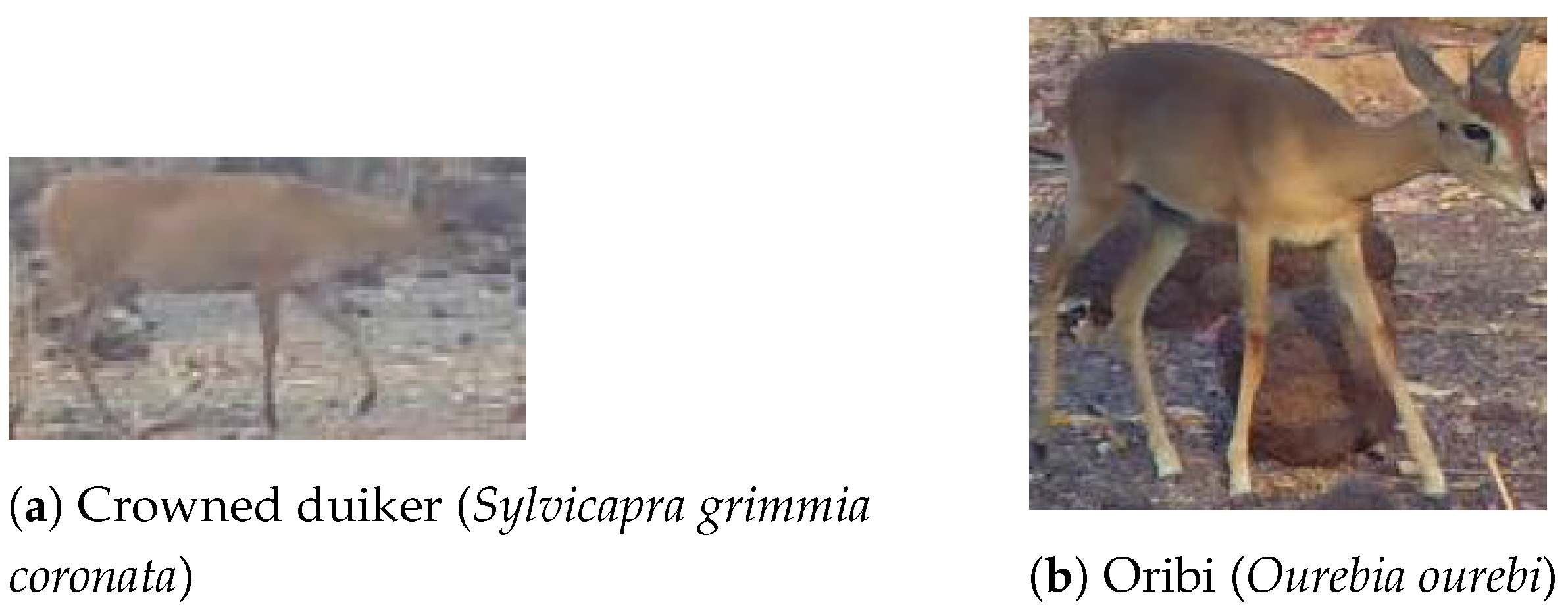
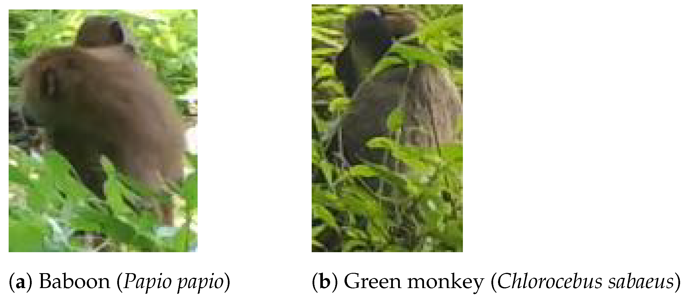
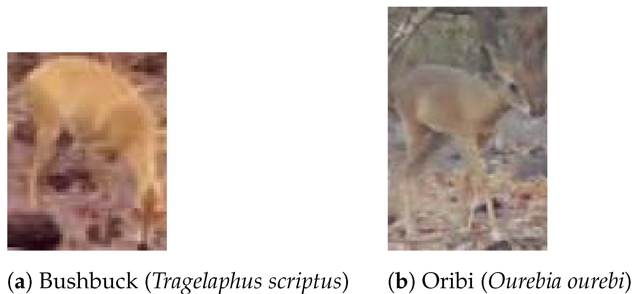
• Environmental/Imagery challenges: Images obtained from camera traps may be very different from the generic images collected from the internet that are widely used when constructing benchmark datasets. These differences include images with much lower quality, incomplete objects, and smaller inter-class differences due to (1) different animals being captured with the same background, or (2) inherently similar appearances across species.
• Presence of distractors: Because our data processing pipeline starts with unlabeled raw videos, we have applied frame selection schemes and an off-the-shelf camera-trap animal detection model in order to produce the cropped images that are input to a classifier. Since we do not have a 100% accurate detector, we observe many cases of false detection—cases where a non-animal object is detected as an animal and, therefore, is considered for classification. Meanwhile, these “distractor” images are typically ignored when using benchmark datasets, and they are also not considered during typical FSL network design.
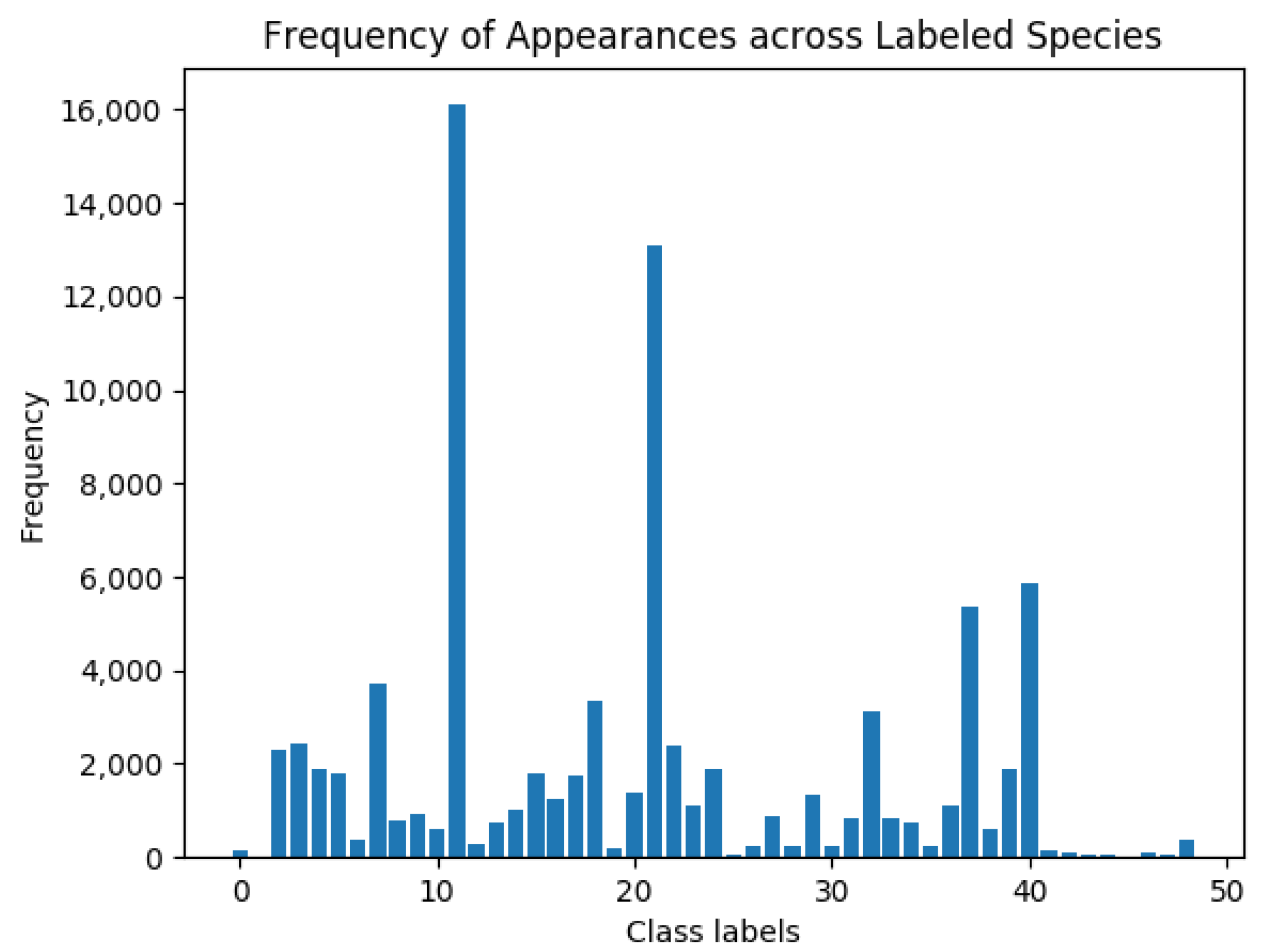
• Unbalanced class distribution: The distribution of animals in nature is inherently unbalanced, which causes some species to appear far more often than others; this has also not been considered in most FSL benchmark datasets.

More detailed descriptions of these challenges can be found in Section 3.2.

To explore these issues, we constructed two datasets from our camera-trap data to reflect these challenges. The first, Senegal-B (benchmark), follows the traditional few-shot evaluation protocol, and is used to create a straightforward comparison to isolate the issues related to our environmental and imagery challenges. The second, Senegal-I (implementation), mimics a real-world scenario where the user annotates a few images per species and builds an automated classification tool for the rest of the data. The second dataset incorporates the latter two challenges that have not been considered by benchmark datasets. Details of these two datasets can be found in Section 3.3.

Through preliminary explorations of these two datasets, we found that performance on a benchmark setting does not necessarily reflect a network’s true usefulness in the more complex implementation settings [4]. In short, our main contribution is to put the theory of FSL to the test by exploring its role in addressing a real-world problem with the extra challenges that are present. In this paper, we expand on our previous work [4] to make further contributions:

• introducing additional evaluation protocols in the implementation settings to systematically quantify a network’s usefulness under the aforementioned challenges;
• conducting more comprehensive experiments with more FSL networks, and confirming our assumption that benchmark testing performance does not necessarily reflect real-world usefulness;
• performing additional experiments that explore the real-world impact, considering both factors involved in network design and factors not previously considered in benchmark testing.

2. Background

2.1. Species Classification for Camera-Trap Videos/Images

Our overall project aims to explore the ecological basis of hunting and meat sharing in female savanna chimpanzees [5,6] by estimating the population density of several species that are hunted by chimpanzees. The research team has placed hundreds of motion-triggered camera traps across two major locations in Senegal—Assirik and Fongoli. The current state of data collection can be found in

Table 1. Data shipments we have received.

Shipment	Videos	Images	Size (GB)	Cameras
1	2998	106,283	187	48
2	25,606	10,433	1304	110
3	3489	2392	132	31
4	6894	1410	284	37
5	11,523	356	642	39
6	4759	1354	167	22
Total	55,269	122,228	2716	287

.

To conduct population estimation from the tens of thousands of videos we have captured, we need a system that (1) samples frames from videos, (2) detects and localizes animals in each frame, and (3) classifies each detected animal into its species. Various studies from both ecology and machine vision researchers have begun to address the detection and classification problem. Norouzzadeh et al. [7] utilize a deep neural network to extract animal species information directly from the frames. Pavlovs et al. [8] implement both one-stage detectors (RetinaNet) and two-stage detectors (Faster R-CNN) and compare their performance when trained to detect and classify two ungulate classes—deer and wild boar. In addition, Zhang et al. [9] focus on improving animal detection performance with cluttered backgrounds by incorporating more temporal information. Singh et al. [10] also address the problem of animal detection with complex backgrounds by constructing background models under different lighting conditions throughout the day. In this paper, we will limit our discussion to only the classification part.

2.2. FSL Methods

Few-shot learning aims to adapt to a new task with a small amount of labeled data, and researchers have explored multiple ways of achieving that goal. Under the FSL philosophy, the networks are usually trained with a relatively large amount of data and then tested with new tasks. Due to the scope of this paper, which is focused on the application of animal species classification, we will mainly discuss few-shot classification studies. However, it should be noted that FSL has also been applied in several other fields, such as detection [11] and image segmentation [12].

For few-shot image classification, the testing setup is usually described as an N-way K-shot classification problem. “N” denotes the number of classes and “K” denotes the number of support images per class. Under this framework, it is assumed that the user would only need to label K images per class (to create a set of support images) for the FSL algorithm to perform the classification. Each of the small sample problems, which consist of N classes, K support images (per class), and several query images (which are assumed to be unknown) is called an “episode”.

In general, an FSL algorithm usually contains two parts—a feature extractor and a decision maker. In this paper, we categorize them into two major methods. Metric learning aims to learn a robust feature extractor so that images from new classes will also follow certain rules in the feature space (e.g., images from the same class will be closer in feature space). Meta-learning aims to find a “best learner”, usually in the form of a set of hyper-parameters, so that a model can be trained with a minimum amount of data when a new task arrives. Note that these two methods are not mutually exclusive, as many algorithms combine both to achieve better results.

For metric learning, after a robust feature extractor is obtained, the classification stage is rather straightforward. The Matching Network [2] and ProtoNet [13] can be considered as two representatives of metric learning. During testing with new classes (or new tasks), Matching Network compares the cosine similarity of an unknown image’s feature and the few labeled samples (support images), and assigns the closest match as the classification result. Similarly, ProtoNet compares the Euclidean distance between the unknown image’s feature and the mean feature computed using the few labeled samples. Some other metric-learning algorithms include RFS [14], which uses logistic regression fitted with the support images as the classifier, and Baseline [15], which uses a single linear layer followed by the softmax function as a classifier, also fitted with the support images.

One benefit of this type of decision rule is that it can be easily changed to fit a user’s desired applications. For example, a network that is trained to perform 5-way classification can be easily modified to perform 6-way or 11-way classification, without needing to re-train the entire network.

For meta-learning, the idea is to find a network that can be trained with very little data. This is usually achieved by having an “outer” optimizer on the hyper-parameters of the network. Under one “meta-training” step, the network is trained to classify the N classes using provided support images (a process known as “inner” training), and then it performs the classification task on unknown query images. The performance of the network on those queries will be used to compute a task loss to measure how well the network is at learning to classify, and this loss is used to update the hyper-parameters of the network. MAML [16] is one of the earliest works that introduced this idea.

In more recent work, many researchers choose to apply both metric learning and meta-learning. For example, $e^{3}bm$ [17] has two training stages: a “pre-training” stage to train a feature extractor, and a “meta-training” stage to train an ensemble of classifiers using the meta-learning philosophy. However, from an implementation perspective, one problem of this kind of meta-learning method is that it does not generalize well; for example, if a user wants a six-way classifier, then the meta-training process must be repeated.

As the field has been growing rapidly, there are many other innovative FSL methods. For example, Xiong et al. [18] use a graph neural network (GNN) to extract edge features and compute edge similarity matrices to achieve few-shot classification. Jiang et al. [19] propose a region-graph transformer (RGTransformer) to capture structural relationships between regions of the image.

2.3. FSL Benchmark Datasets and Evaluation Protocols

Popular few-shot learning datasets include Omniglot [20], primarily designed for a character recognition task, and mini-ImageNet [2], a subset of ImageNet primarily designed for a general image classification problem. There also exist several alternatives to construct a few-shot dataset from ImageNet, including tiered-ImageNet [21] and better-tiered-ImageNet [22].

For testing and evaluation, the episode-based method is now the dominant protocol after being proposed in [2] and further elaborated upon in [23]. Essentially, each “N-way K-shot” episode mimics one FSL problem that involves N-way classification, given K labeled images per class. For example, to construct a “5-way 5-shot” episode, one will first sample five classes out of all possible classes, and then sample five images per class to be considered as labeled images; this set of $5\times 5=25$ images are known as the “support set”. Then, several images per class will be sampled to serve as the “unknown images to be classified”. This set of images is known as the “query set”. The images in the query set will not overlap with images in the support set. The number of images in the query set may vary, but we have found that 15 images per class is commonly used. The FSL method then uses the knowledge of the support set to classify the query set by, for example, training a lightweight model or applying a nearest-neighbor classifier. The top-1 accuracy of this episode will be recorded, and the process will be repeated many times to ensure reliable results.

Two things to highlight are that (1) current FSL evaluation protocols sample an equal number of query images per class, and (2) current protocols do not consider the case where an image may not belong to any of the N classes. In Section 3.3.2, we present a new dataset using real-world camera-trap data, which differs in these two aspects from benchmark datasets. We then propose additional evaluation protocols to quantify a network’s performance under these challenges. In doing so, we hope to illustrate the difference between benchmark datasets and real-world data, and encourage researchers to look beyond optimizing networks solely for benchmark purposes.

2.4. Applied FSL

Many researchers have already started to explore the gap between benchmark datasets and realistic problems. Chen et al. [15] argued that despite disjoint classes, training and testing on the same dataset does not necessarily replicate the domain difference likely to be observed in real-world problems. The authors then created a cross-domain testing case by training few-shot learning networks using a benchmark dataset (mini-ImageNet) and testing on a fine-grained classification dataset (Caltech-UCSD Birds 200 [24]) re-partitioned to fit the few-shot learning benchmark style. In [22], the authors criticized current benchmark datasets for lacking realistic meaning between classes in each sub-task (i.e., an episode). They proposed a relevance measure between classes using semantic structures, and used that measure to create a dataset with more relevant class sampling.

Many researchers have also investigated FSL applications to real-world problems. Nuthalapati et al. [25] focused on agricultural application of plant and pest classifications, and set up an experiment for various cross-domain settings. Zhang et al. [26] used FSL techniques for rolling bearing fault detection using vibration patterns. Yoo et al. [27] compared several FSL methods for the task of classifying rare retinal diseases using OCT images, including prototypical network [13], Siamese network [28,29], and data generation with CycleGAN [30]. Prabhu et al. [31] applied FSL for dermatological disease classification; they also point out the unbalanced class distribution between common and rare diseases, and proposed to use mean per-class accuracy to quantify a network’s performance across classes. Wang et al. [32] utilized few-shot learning to be able to add new classes for the task of synthetic aperture radar (SAR) automatic target recognition (ATR).

In addition to classification tasks, FSL has also been explored in other fields. Zhong et al. [33] used FSL to improve an image retrieval task with remote sensing images by proposing a loss function designed to optimize mean average precision (mAP). Karami et al. [11] trained a detection network using FSL techniques to fit the task of plant detection from aerial photographs.

3. Materials and Methods

Real-world data are very different from benchmark datasets. Due to factors such as camera condition, environment, and target class of interest, real-world data may pose challenges that are not addressed in benchmark datasets. The overall experiment in this paper is to train FSL networks using publicly available datasets, and evaluate their performance with our data, where more realistic challenges are present.

We begin, in Section 3.1, by giving a big picture of our data collection and processing pipeline. In Section 3.2.1, we describe the three major challenges with our data: environmental/imagery challenges, presence of distractors, and unbalanced class distribution. Two testing datasets based on our data are then introduced in Section 3.3 to reflect these challenges. We also introduce additional evaluation protocols and performance metrics to reflect these challenges. Finally, in Section 3.4, we present the details for the networks we use and the training settings.

3.1. Data Description

Our data are taken from motion-triggered camera traps around two major sites in Senegal—Assirik and Fongoli. As of now, we have received 6 data shipments, totaling 55,269 videos and 122,228 images from 287 camera locations in a mosaic savanna woodland environment; the entire data volume is 2716 GB (gigabytes). Details of our data collection can be seen in Table 1; note that the term “CT days” (camera-trap days) is counted as days between when a camera started to record and when it recorded its last video/image. We evenly sample one frame per 3 s (90 frames), and apply an off-the-shelf animal detector https://github.com/microsoft/CameraTraps (accessed on 1 May 2022)) to obtain 181,685 unlabeled bounding boxes of potential animal sightings.

For this paper, we consider 114 camera locations from data shipments 2 and 3, and randomly sample about 8000 bounding boxes out of the total 63,569 detected bounding boxes from these two data shipments. We have labeled these 8000 images to serve as a representative subset of our data. These images include both correctly detected animals as well as false positives that were mis-detected.

3.2. Challenges

3.2.1. Environmental/Imagery Challenges

Unlike many benchmark datasets that obtain generic images from the internet, our data that was captured in the wild suffers much more from poor image quality. Such factors include, but are not limited to: low resolution: due to animals being detected far from the camera; occlusion: due to plants or other animals; incomplete animals: due to animals being detected too close to the camera or at the edge of the frame.

Additional challenges lie within the general context of the data, namely, separation between classes, and variation within the same class. We observed many cases of small inter-class (between class) separation. The cause of such small separation may be the result of (1) inherent similarity (build, color, etc.) in species or (2) similar backgrounds, since our data came from stationary camera traps in the same region.

Here, Figure 1 shows one case of small separation between classes due to the similar build and color of the two animal species, and Figure 2 shows another case due to similar background. The challenge is even more significant with lower-quality images, as shown in Figure 3. For all three figures mentioned above, the images retain their original resolution from camera trap videos. The low image quality is the true reflection of our real-world data.

In the end, the aforementioned challenges can be seen as inevitable whenever applying FSL to a new environment or new task, and each of the FSL applications cited above [25,26,27] face their own environmental and imagery challenges. However, the challenges discussed next are less well-investigated, as many people tend to view FSL classification as a stand-alone problem, without considering its context within a large processing pipeline or its general data context.

3.2.2. Presence of Distractors

As stated in the Background section, to compare results for few-shot learning networks, most benchmark datasets simplify the problem. For each episode of the “N-way K-shot classification” task, all the queries, or unknown images, are selected from the N classes. This means these algorithms do not have to consider that an image might not belong to any of the classes. However, real data does not fulfill this assumption. Our data contains many images not belonging to any of the species we are interested in. Most of these images are caused by false detections of background objects that are not animals. In addition, a few of these images are of other animal species outside of our research scope.

Another key issue to note is that these “distractor” images do not actually belong to just a single class, as they do not necessarily share common features. Hence, the problem is more “identify images not belonging to any class” instead of “identify images that belong to a single ’distractor’ class”.

3.2.3. Unbalanced Class Distribution

FSL evaluation protocols also assume an equal number of images per class among the unknown images, as stated in Section 2.3. However, that assumption does not always hold with real-world data. As already mentioned by [31], real-world data are often long-tailed, which means that there are usually some classes with more observed cases, as well as other classes with fewer cases. During the initial screening and labeling of our data, we randomly selected 8000 images to be labeled and found a heavily unbalanced class distribution, as seen in

Table 2. Images of each species used as query for our implementation-style dataset (Senegal-I).

Species	Images	Species	Images
Baboon	1624	Hartebeest	21
Buffalo	566	Oribi	10
Bushbuck	46	Patas monkey	54
Duiker	212	Roan antelope	167
Green monkey	247	Warthog	245
Guineafowl	1831	Distractors	2586

. For example, the Guinea baboon is more common and represented in 1624 images, while the rarer patas monkey is captured in only 54 images.

3.3. Dataset Formation

Given these challenges, we formally evaluate a network’s performance on our data by constructing two datasets from our images. Senegal-benchmark (Senegal-B) mimics a benchmark evaluation protocol and enables us to focus on easy and straightforward comparisons between networks under our environmental challenges. In contrast, Senegal-implementation (Senegal-I) enables an in-depth exploration of the differences between benchmark datasets and potential real-world implementation, specifically the presence of distractors and unbalanced class distributions.

3.3.1. Dataset 1: For a Benchmark-Style Evaluation

To begin, we constructed a small dataset containing a few images per species, entitled Senegal-B (B stands for benchmark). The number of images per species can be found in

Table 3. Images of each species for our benchmark-style dataset (Senegal-B).

Species	Images	Species	Images
Baboon	108	Hartebeest	25
Buffalo	74	Oribi	22
Bushbuck	126	Patas monkey	30
Duiker	53	Roan antelope	97
Green monkey	99	Warthog	83
Guineafowl	86

. Senegal-B follows the typical FSL benchmark evaluation protocol for straightforward comparison, and uses our images to reflect the aforementioned imagery/environment challenges. The main purpose of this dataset is to compare a network’s cross-domain performance when it has been trained with publicly available data but applied to our specific environment.

In selecting images, we have also taken an extra step to eliminate visually similar images to make the variations within each class larger; e.g., if an animal stays in the same spot and is detected multiple times, only one image will be included. To apply our benchmark-style evaluation protocol, we apply 5-way, 5-shot settings with 15 query images per species. We conduct each testing process by randomly sampling 300 episodes. The process is repeated five times with different random seeds.

3.3.2. Dataset 2: For an Implementation-Style Evaluation

For the second dataset, we mimic a real implementation process of few-shot learning, and name it Senegal-I (I stands for implementation). Instead of carefully selecting images with reasonable quality and avoiding visually similar images, we randomly sampled and labeled 8000 detected animals from shipments 2 and 3 of our data, only excluding those already selected for Senegal-B. Therefore, Senegal-I and Senegal-B have disjoint image sets. This is important because in using Senegal-I for testing, we will treat all 8000 images as unknown queries, and attempt to classify them based on a support set selected from Senegal-B. In addition, while there may exist visually similar images due to animals re-appearing in the same camera within the Senegal-I set, there are no exact duplicates.

As mentioned in the second part of the challenges with real data (i.e., “differences”), several assumptions made in benchmark datasets do not hold with non-curated data. To begin with, unknown image queries do not follow a nicely balanced distribution between classes. As can be seen from Table 2, some of the species are more frequently detected than others. In addition, a testing episode in the benchmark datasets’ evaluation does not consider images that do not belong to any of the classes. However, in our case, we observe about 30% distractor images that do not belong to any of the classes. These images are often background objects, such as branches or rocks that have been mis-detected as an animal. As these images are from multiple different object types, they do not share inherently similar features to be regarded as one single class.

As mentioned earlier, the traditional few-shot learning evaluation protocol does not consider distractor images (images not belonging to any class) and always assigns a class to an unknown image. Therefore, for this implementation-oriented dataset, we need an extra step in our evaluation protocol to decide whether images should be classified into one of the classes or not. In contrast to the benchmark evaluation protocol, we use a different evaluation protocol on this dataset (Senegal-I), which we call the implementation evaluation protocol.

First, in the implementation evaluation protocol, we mimic an implementation scenario where all classes and all images need to be considered at the same time. We select 10 images per class from the relatively higher-quality Senegal-B dataset, and treat them as the support images for each class. The 8000 images from the Senegal-I dataset are then treated as queries. Second, since we have many distractor images, an additional decision rule must be applied. In this paper, we choose to use a group of k-nearest neighbor (KNN) classifiers to serve as the decision rule for eliminating distractor images; the details of the KNN rules used can be found in Section 4.1.2.

For comparing results on this dataset, we will examine two performance metrics, each corresponding to one of the aforementioned challenges (presence of distractor and unbalanced class distribution). To quantify a network’s ability to reject distractor images and to admit correct animal images, we define the following true positive rate (TPR) and false positive rate (FPR), and plot them to form the ROC curve.

• False positive rate (FPR) is the number of distractor images that pass the decision rule divided by the total number of distractor images. The FPR measures a network’s effectiveness at eliminating distractor images.
• True positive rate (TPR) is the number of animal images that passes the decision rule and are correctly classified, divided by the total number of animal images. TPR measures a network’s effectiveness at admitting correct animal images. Due to the very low quality on some of the animal images, we do not expect all animal images to be classified. In other words, we do not expect the TPR to reach 100%.

Note that our definition of TPR reflects the fact that we are not considering traditional binary classification, and this influences the ROC curve as well.

To quantify a network’s classification accuracy across classes, we use the top-1 match to compute the mean per-class accuracy (MCA), as used in [31]. The MCA computes a top-1 accuracy for each class separately, and then forms the arithmetic mean across classes; this way, classes with more images are not favored in the accuracy comparison. It is expressed formally as

$$MCA=\frac{1}{C}\sum _c\frac{{\sum }_{t=1}^{T_c}[{\widehat{y}}_{top1}^t=y^t]}{T_c}$$

(1)

for a dataset with C classes and $T_c$ samples in each class; the ${\widehat{y}}_{top1}^t=y^t$ is an indicator variable that is 1 only if the top-1 prediction is correct.

3.4. Network Training Settings

For our experiment, we will examine the performance of various FSL algorithms on our data. We have selected nine FSL networks: ProtoNet [13], RFS [14], Baseline and Baseline++ [15], R2-D2 [34], $e^{3}bm$ [17], RENet [35], SSL-FEW-SHOT [36], and P > M > F [37]. These selections include both classic algorithms that have paved the way, as well as more recent ones that have achieved better performance on benchmark datasets. As we follow the FSL philosophy of minimizing human labor when labeling new data, we will train each network with a publicly available dataset, but will test on our data, Senegal-B and Senegal-I, each corresponding to certain real-world challenges. Since the public training data and our own test data inevitably have different environments and different classes, this is inherently a cross-domain problem. We will see the effect of domain gaps when we compare the results.

In this paper, we choose two public datasets for training. The first one is the mini-ImageNet dataset, which is designed for few-shot learning. We will use the train/val split proposed in [23] https://github.com/gitabcworld/FewShotLearning (accessed on 1 August 2022), which provides 38,400 images from 64 classes for training (600 images per class). The second dataset we use is a camera-trap dataset named Snapshot Serengeti [38]. For convenience purposes, we may refer to this dataset as “S.S.” in places such as tables or plots. To date, the Snapshot Serengeti project has collected more than 7 million images from camera-trap sites across Tanzania’s Serengeti National Park, totaling more than 5710 GB of data https://lila.science/datasets/snapshot-serengeti (accessed on 1 August 2022). These images are then labeled by thousands of “citizen scientists” with the help of an interactive species identification tool https://www.zooniverse.org/projects/zooniverse/snapshot-serengeti (accessed on 1 August 2022). In this paper, we only utilized the first four seasons from the Snapshot Serengeti dataset, which contains 1243 GB of data. We extracted 85,542 bounding boxes in total using official metadata, which belong to 48 species. The distribution of these bounding boxes can be seen in Figure 4.

As we can see, the class distribution is very unbalanced. For example, class 11 (elephant) has 16,101 images, whereas class 12 (aardvark) has only 297 images. If we directly take all these data into training, the result might be heavily biased towards the few classes with an overwhelming number of images. Therefore, we establish a more balanced training set with 8558 images in total, where we randomly select 200 images if a species has more than 200 images, and take all available images if a species has fewer than 200 images.

Unless specified, we choose ResNet-12 as the backbone for the feature extractor, and train with a 5-way 5-shot setup. For few-shot training, all networks use cross-entropy as the loss function. In addition, RENet [35] uses a combination of an “anchor loss” based on an additional fully connected layer, as well as a “metric loss” based on cosine similarity; both are still cross-entropy losses. As for the decision rules used to obtain a prediction during training, four of the nine networks use a simple closest neighbor rule. Among these three, ProtoNet [13] and SSL-FEW-SHOT (SSL for short) [36] use Euclidean distance, while P > M > F [37] and Baseline++ [15] use cosine similarity. Baseline [15], RFS [14], and R2-D2 [34] all use a form of linear classifier for their decision rule, while RENet uses a novel cross-correlational attention (CCA) module and $e^{3}bm$ [17] uses a more complex ensemble of classifiers. To evaluate the networks, we use a compute server with four NVIDIA TITAN Xp GPUs (12 GB memory each) for both training and testing.

Three networks ($e^{3}bm$, SSL, and P > M > F) require a pre-trained network. For result reporting in tables and graphs, the dataset used for pre-training will be indicated in parenthesis. $e^{3}bm$ [17] uses a few-shot dataset for pre-training; in our case, therefore, we use either Mini-ImageNet or Snapshot Serengeti (S.S.) for pre-training. SSL-FEW-SHOT [36] uses two larger subsets of ImageNet for its self-supervised pre-training (which means no labels are provided, and only the images themselves are used); Mini80 includes 48,000 images from 80 classes, and ImageNet900 (abbreviated as IN900 in tables and graphs) includes about 1 million images from 900 classes. P > M > F [37] uses a pre-trained vision transformer DINO [39]. It is also trained using self-supervised learning on ImageNet, but since it does not vary, we will not specify it.

4. Results and Discussions

In this section, we conduct testing on each of our datasets, Senegal-B and Senegal-I, to determine the usefulness of an FSL network when it faces the more realistic challenges our datasets impose.

The section is organized as follows. First, we explore each of the networks on each individual dataset. In Section 4.1.1, we report the networks’ performance on Senegal-B using top-1 accuracy. In Section 4.1.2, we report the networks’ performance on Senegal-I using the ROC curve and an MCA score, as described in Section 3.3.2. Then, in Section 4.1.3, we present a discussion about the gap between the benchmark and implementation settings by comparing the results across the two datasets.

Next, we explore individual factors that could influence a network’s performance under more realistic implementation settings. In Section 4.2, we discuss the assumption that self-supervised pre-training with extra data is the key to a robust feature extractor. Finally, in Section 4.3, we consider additional design choices associated with applying FSL networks in the implementation setting.

4.1. Overall Comparison of FSL Network Performance under Challenging Environments

4.1.1. Results Part 1: Benchmark-Style Evaluation

For testing with Senegal-B (benchmark-style), we follow the traditional FSL episode construction and randomly create 3000 episodes, each representing a 5-way 5-shot problem with 15 queries, and we report the top-1 accuracy. Using the benchmark-style dataset and top-1 accuracy enables a straightforward comparison among the underlying FSL networks in the context of our environment, which can be considered to be a cross-domain FSL problem.

We also compare here the results of training on two datasets: a subset of Snapshot Serengeti and mini-ImageNet. The goal is to understand the implications of training data selection on FSL performance. Recall that the Snapshot Serengeti training set we constructed (49 classes, 8558 images) is smaller than mini-ImageNet’s training set (64 classes, 38,400 images); Snapshot Serengeti also has less variation within class when compared to mini-ImageNet, because its images are taken from stationary cameras rather than internet images from various sources. However, Snapshot Serengeti is more similar to our data, both because it has more similar camera settings (stationary camera traps) and it has a similar classification problem (animal species classification, albeit different species).

The results are shown in

Table 4. Top-1 accuracy (%) when trained on mini-ImageNet (mini-I) and Snapshot Serengeti (S.S.) and then tested on Senegal-B. The performance of each network when tested on mini-ImageNet provides a reference for a typical benchmark dataset and setting.

Network	Train on Mini-I Test on Mini-I	Train on Mini-I Test on Senegal-B	Train on S.S. Test on Senegal-B
ProtoNet [13]	74.19	62.16	60.97
RFS [14]	79.74	62.96	71.56
Baseline [15]	76.18	67.54	71.98
Baseline++[15]	66.36	54.39	56.49
R2-D2 [34]	74.35	63.93	67.63
e3bm [17] (pre: Mini)	80.60	67.01	68.59
e3bm [17] (pre: S.S.)	-	-	59.69
RENet [35]	82.23	69.81	66.62
SSL [36] (pre: Mini80)	81.21	66.69	71.81
SSL [36] (pre: IN900)	90.79	71.90	76.32
P > M > F [37]	97.30	92.10	92.10

, where the performance of each network when tested on mini-ImageNet is also shown, to provide a reference for how well these FSL networks perform on typical benchmark datasets and settings.

When comparing the networks’ performances, we see that P > M > F significantly outperforms all other networks in all scenarios. One potential reason for this may be the advantage of using a vision transformer backbone that was pre-trained with a large amount of data. Behind P > M > F is SSL-FEW-SHOT, which also employs self-supervised learning with extra training data. We will discuss more about pre-training with extra data in Section 4.2.

Next, we look at all other networks that do not use extra training data ($e^{3}bm$’s pre-training stage is limited to the same FSL dataset and, thus, it does not involve extra data). First, we see that Baseline++ has the worst performance when trained and tested on Mini-ImageNet; Baseline++ also performs the worst when tested on our Senegal-B dataset, regardless of which training dataset is used. However, the ordering of the other networks is not consistent between the two testing datasets. RENet and $e^{3}bm$ are the two best-performing networks on the mini-ImageNet benchmark, but they are not the best on Senegal-B (where Baseline and RFS perform best).

As a result, it appears difficult to extrapolate results from one dataset to another. Network improvements that result in better performance on mini-ImageNet may not lead to similar improvements on our datasets.

Next, we consider the implications of the training data by comparing the columns in Table 4. To begin with, as indicated by the bold numbers, six out of the nine networks (RFS, Baseline, Baseline++, R2-D2, $e^{3}bm$, SSL) performed better when trained with Snapshot Serengeti than when trained with mini-ImageNet. ProtoNet and RENet are the only networks that performed better when trained on mini-ImageNet than Snapshot Serengeti, while P > M > F had equal performance in both cases.

Based on these observations, we conclude that generally, training on more similar data is likely to be helpful when applying FSL to a cross-domain problem such as ours. However, for ProtoNet, having a larger, more extensive training set leads to better cross-domain performance. Moreover, the feature extractor of P > M > F, whose backbone vision transformer was pre-trained on an impressive amount of data, provides a powerful framework for FSL learning in general.

In addition, we see that when trained on mini-ImageNet and tested on our Senegal-B dataset, overall these networks do not have as high a top-1 accuracy as when tested on mini-ImageNet. This indicates that our Senegal-B is a more difficult dataset overall.

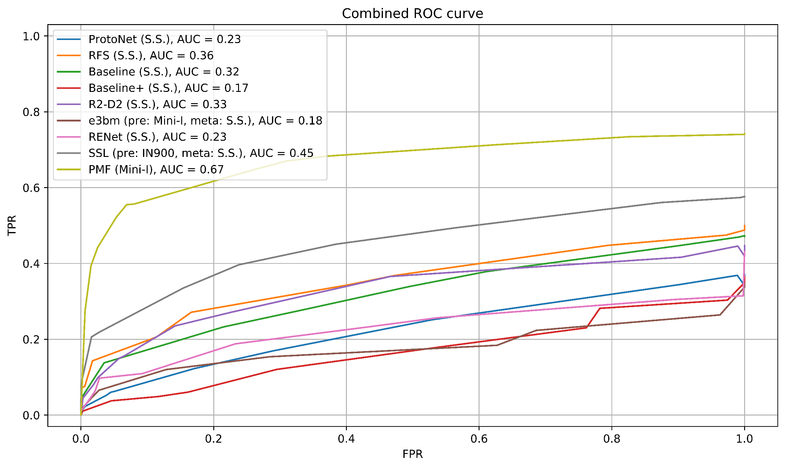
4.1.2. Results Part 2: Implementation-Style Evaluation

For testing with Senegal-I (implementation-style), our goal is to quantify and compare the performance of different underlying FSL networks with the additional challenges of the presence of distractors and an unbalanced class distribution. We will use the two performance metrics described in Section 3.3.2.

The first metric is an ROC curve that quantifies a network’s ability to reject distractors and to correctly classify admitted images. To generate these ROC curves, we implement various k-nearest-neighbor (KNN) decision rules with different Ks and thresholds M. Consider the example of K = 5 and M = 3—for each query (unknown) image, we find the closest five (K) support images in the feature space. The image is only classified if at least three (M) out of these five nearest neighbors are from the same class, in which case this class will be assigned to the query image. This way, for each K and M pair, we calculate a TPR and FPR based on our aforementioned definitions, and we plot an ROC curve that describes the TPR/FPR at different operating points. To reduce confusion and improve visual clarity, we consolidate all the points into one “best” ROC curve. Because of our definition of TPR, the ROC curve should not be interpreted the same as an ROC curve of a binary classification problem.

The second performance metric, mean cross-class accuracy (MCA), has been proposed by [31], and aims to solely focus on a network’s ability to perform the task across classes. Additional details of these two performance metrics can be found in Section 3.3.2.

To begin with, we compare each network’s performance when trained with mini-ImageNet against when trained with Snapshot Serengeti. The MCA scores for each network are reported in

Table 5. MCA (mean cross-class accuracy) when trained with mini-ImageNet (mini-I) and Snapshot Serengeti (S.S.), and then tested on Senegal-I.

Network	Train on Mini-I Test on Senegal-I	Train on S.S. Test on Senegal-I
ProtoNet	21.70	21.20
RFS	27.70	35.00
Baseline	27.20	35.80
Baseline++	24.30	28.80
R2-D2	22.30	31.10
e3bm (pre: Mini-I)	24.80	29.90
e3bm (pre: S.S.)		33.10
RENet	27.00	37.80
SSL (pre: Mini80)	33.90	41.00
SSL (pre: IN900)	40.50	46.60
P > M > F	70.70	46.80

. As was the case for Senegal-B in Table 4, we observe that most networks, except for P > M > F and ProtoNet, perform better when trained on Snapshot Serengeti. At first glance, it may seem that the MCA is quite low. However, considering that the underlying problem is unbalanced 11-way classification both with difficult environments and a large number of distractors (that do not belong to any class), these low numbers are reasonable.

Next, detailed ROCs for each network are shown in the Appendix A, Figure A1, when each is trained on either mini-ImageNet or Snapshot Serengeti. The best results for each network are shown in Figure 5, where the legend indicates for each network which training scenario performed best. Our observations are similar to above. Except for P > M > F, all other networks achieve better performance in the implementation setting when trained with Snapshot Serengeti instead of mini-ImageNet.

4.1.3. Discussion: Performance Difference between Benchmark and Implementation Settings

Here, we discuss detailed findings regarding individual networks’ performances across benchmark settings and implementation settings. This explores whether using benchmark settings in general enables meaningful conclusions to be drawn about applying these networks to our real-world problem.

First, as previously observed on Senegal-B (Table 4), ProtoNet trained with mini-ImageNet outperformed its counterpart trained with Snapshot Serengeti. However, when tested with the more realistic Senegal-I, we observed mixed results (Table 5 and Figure A1e). Although it obtained a slightly better MCA when trained with mini-ImageNet, it obtained a better ROC curve when trained with Snapshot Serengeti. Similar results can also be observed with RENet. When tested on Senegal-B, RENet trained with Mini-ImageNet outperforms its counterpart trained with Snapshot Serengeti, but when tested on Senegal-I, RENet trained with Snapshot Serengeti achieved better performance in both MCA and the ROC curve.

Second, the two versions of P > M > F, trained with mini-ImageNet and Snapshot Serengeti, respectively, achieve the same performance (top-1 accuracy) on benchmark settings (Table 4). However, under implementation settings, the network trained with mini-ImageNet performed dramatically better than the same network when trained with Snapshot Serengeti (Figure A1d).

A third interesting finding is made when we compare performance across different networks. For example, RFS and Baseline showed similar performances on benchmark settings (Table 4), with Baseline being slightly better. However, in implementation settings, RFS obtained a significantly better ROC curve than Baseline (Figure 5). Nevertheless, the two networks that come with extra training data (P > M > F and SSL-FEW-SHOT) are still the two best performing networks when applying the implementation settings.

Finally, the case of $e^{3}bm$ [17] is a bit more complicated, as it consists of two training stages—a pre-training stage and a meta-training stage. As briefly mentioned in Section 2.2, its pre-training stage aims to train a general feature extractor, and the meta-training stage trains an ensemble of classifiers with trainable hyper-parameters, so that the classifiers can adapt to a new task easily. To begin with, we observe that during benchmark testing, pre-training with Snapshot Serengeti (S.S.) yields much worse performance than pre-training with mini-ImageNet, regardless of which dataset the meta-training stage uses. However, the same trend does not persist when we test with the more realistic implementation case (see Figure A1c for ROC curves and Table 5 for MCA). For ROC curves, pre- and meta-training with S.S. performed similarly to pre-training with mini-ImageNet and meta-training with S.S., and much better than pre- and meta-training with mini-ImageNet. For MCA, pre- and meta-training with S.S. outperformed the other two completely. We do notice that $e^{3}bm$ performed rather poorly under implementation settings when compared to other methods, and this is discussed further in Section 4.3.4.

The aforementioned observations are all examples where conclusions drawn from results on a benchmark dataset may not be valid for all aspects of implementation.

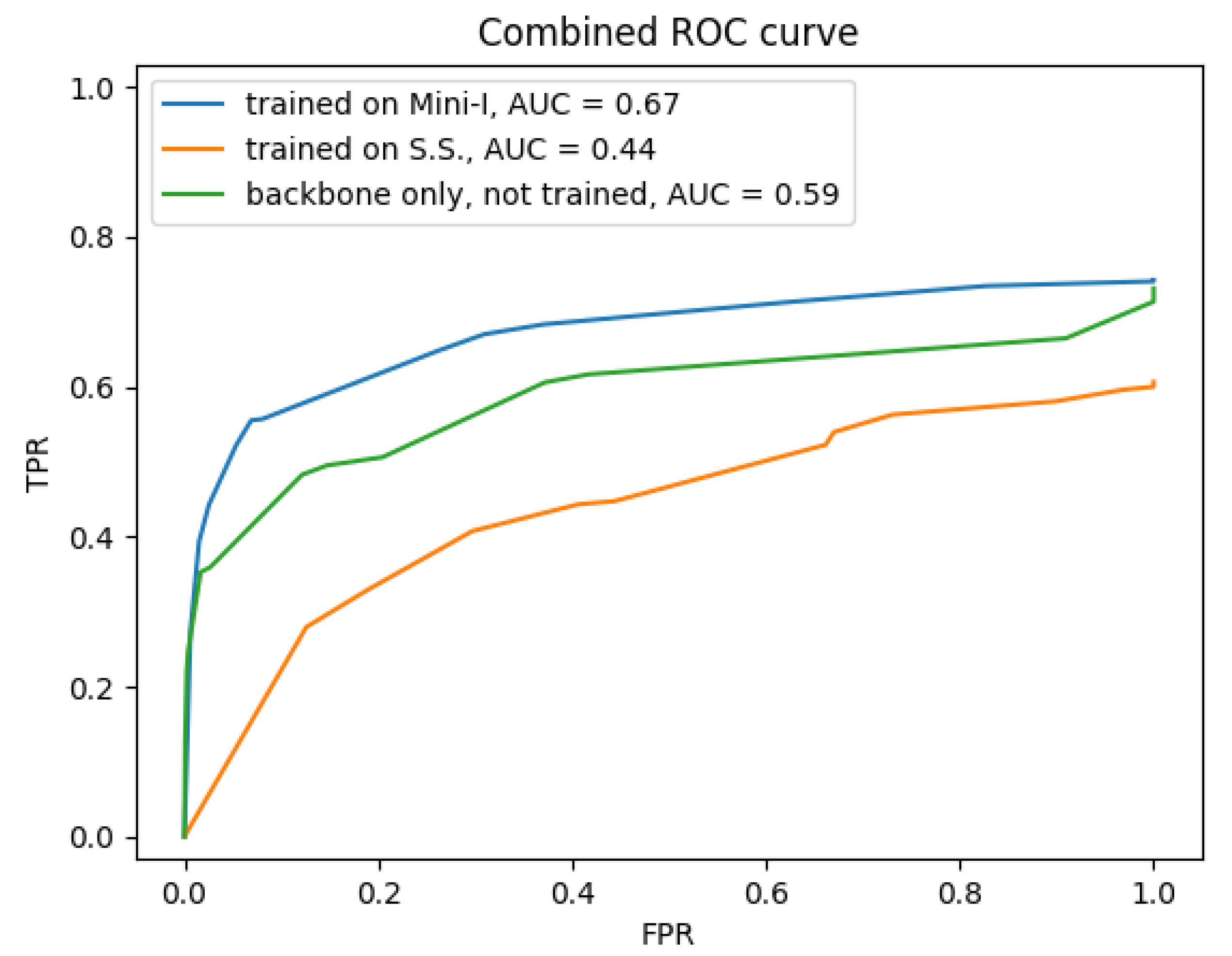
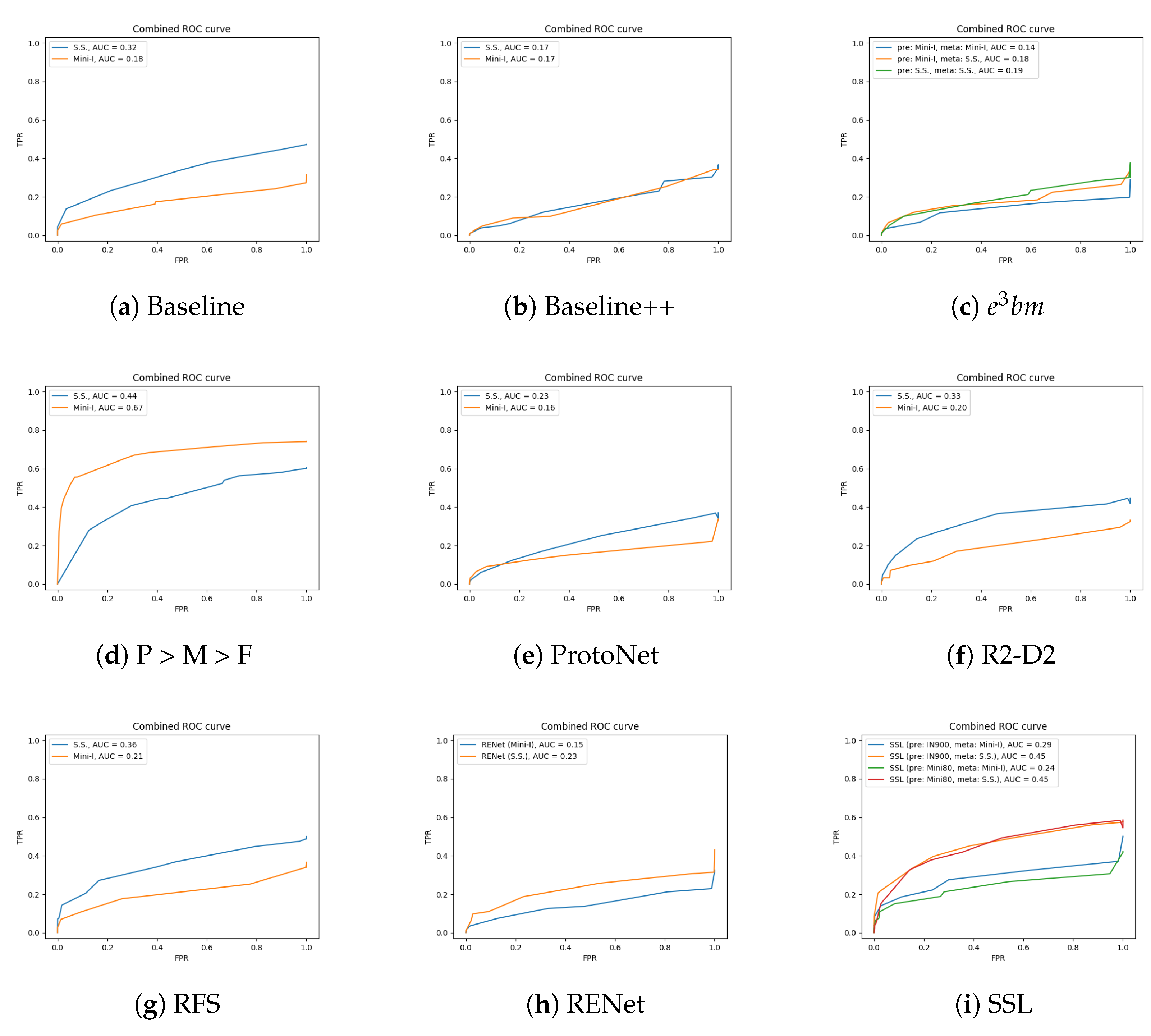
4.2. Benefit of Extra Training Data and an Effective Feature Extractor

It is clear that P > M > F [37] and SSL-FEW-SHOT [36] perform better than all other networks. Our assumption is that extra self-supervised pre-training leads to a more robust feature extractor and, therefore, better FSL performance in real-world data. In this section, we explore this hypothesis.

Unlike most FSL networks, that take a generic ResNet [40] or WRN (wide residual network) [41] as backbone for the feature extractor part, these two incorporate self-supervised learning frameworks as the feature extractor. SSL-FEW-SHOT uses AMDIM [42], which is based on mutual information maximization. P > M > F takes advantage of a more advanced vision transformer (ViT) named DINO [39] as the backbone. The rest of P > M > F is quite straightforward; it uses a ProtoNet-style training process and a simple closest neighbor decision rule. This means its massive performance advantage over the other networks is mostly likely due to the pre-trained backbone.

To demonstrate the effectiveness of the vision transformer backbone, we conduct the same implementation testing using pre-trained DINO as a feature extractor directly, without any further FSL-style training on mini-ImageNet or Snapshot Serengeti. Figure 6 shows the results using the pre-trained backbone compared to training it further with mini-ImageNet or Snapshot Serengeti in FSL style. Compared to the results in Figure 5, we can see that even without any training, simply using the pre-trained vision transformer as a feature extractor still outperforms any other FSL network. This demonstrates the benefit of a powerful feature extractor pre-trained with external data.

This may seem like an unfair advantage in benchmark testing, as none of the other networks use external training data. However, in a real-world setting, we believe it is important to exploit all possible benefits in order to help the end user. In this case, self-supervised pre-training has been shown to be very effective under our implementation settings. It is especially valuable in our cross-domain problem, both because we want to minimize the labeling effort, and because our available training data (Snapshot Serengeti or mini-ImageNet) still have a considerable domain gap when compared to the real-world data.

Another interesting observation regarding P > M > F is that when we train the network further using Snapshot Serengeti, its performance in implementation actually degrades, suggesting that training with a domain-restricted and potentially heavily unbalanced dataset (see Figure 4) may be detrimental to the effectiveness of the general purpose feature extractor. Incidentally, in 2020, Tian et al. [14] have already suggested that a robust feature extractor is all FSL needed. The fact that P > M > F performs so well as a robust general purpose feature extractor further supports this assertion.

4.3. A Deeper Look into FSL Classification in Implementation Settings

In general, the implementation process is straightforward: extract features and compare their similarity to known species classes. However, there are still components that may affect the results. In this section, we consider additional aspects of applying an FSL network to a real-world scenario. Therefore, the experiments here are limited to the implementation settings using Senegal-I.

First, we discuss three design aspects that are not necessary to consider when using a benchmark dataset. The first two focus on how extracted query features (assumed to be unknown) are compared to support features (assumed to be labeled). Specifically, we consider (1) the distance metric used to characterize similarity between features, as well as (2) if additional feature transformations can help the process. The third concerns how the choice of support images affects the performance of networks under more complex implementation settings, which is often ignored when a benchmark dataset is in place. Then, we will then discuss the question “how easily can a network be changed to perform a different task?”.

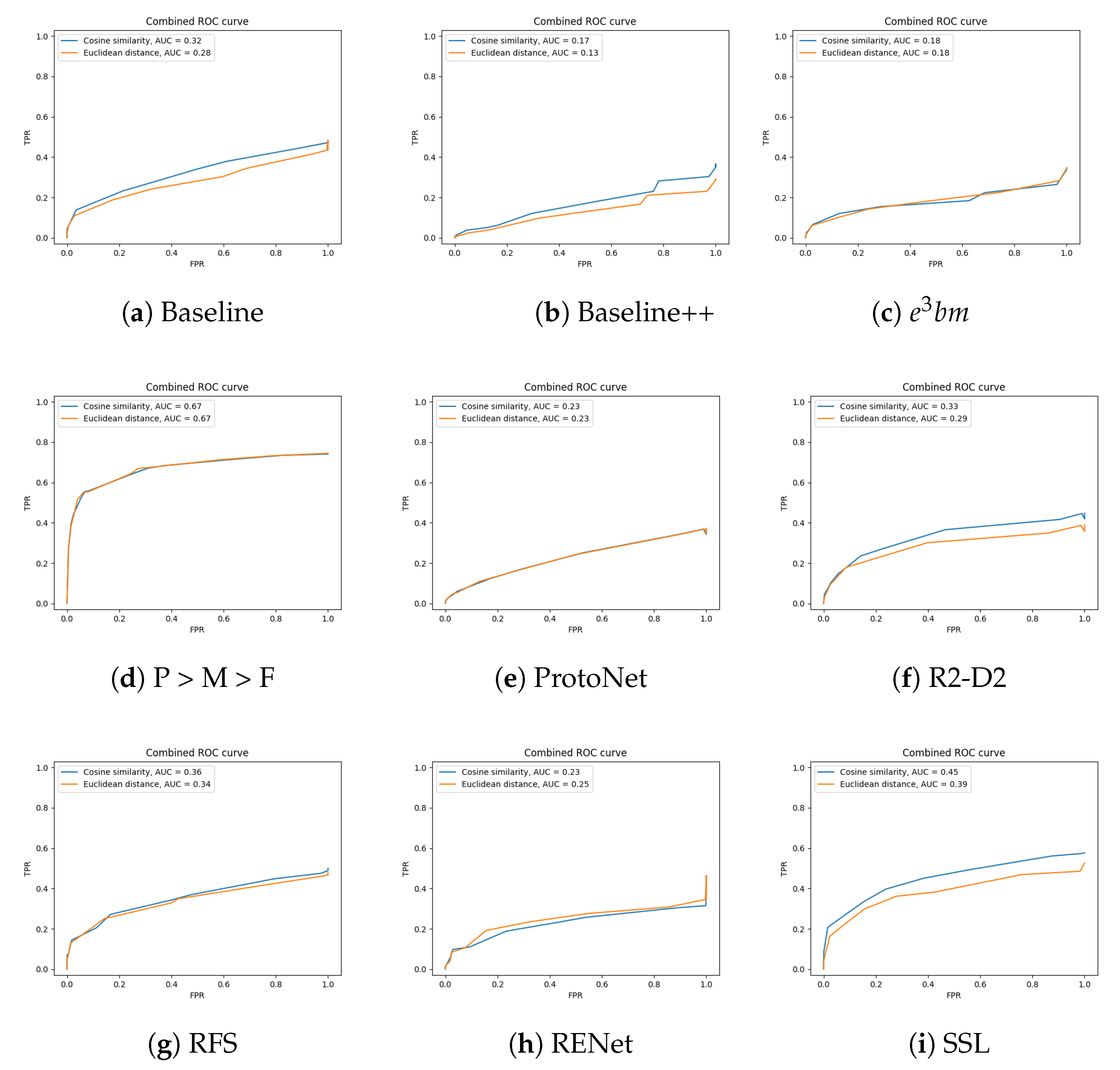
4.3.1. Distance Metrics

The choice of distance metric affects the computation of distances in high-dimensional feature space to compare the extracted features to the features of known classes. Here, we explore the impact of two of the most commonly used distance metrics for feature comparison—cosine similarity and Euclidean distance. For each network, we select its “best-performing” version based on our previous observations using the implementation dataset, and we apply either Euclidean distance or cosine similarity to measure the distance between query and support features.

A summary of the results is shown in

Table 6. AUC (area under curve) when using Euclidean distance and cosine similarity for feature comparison.

Network	AUC Using Euclidean Distance	AUC Using Cosine Similarity
ProtoNet	0.22	0.22
RFS	0.34	0.36
Baseline	0.29	0.32
Baseline++	0.13	0.17
R2-D2	0.27	0.32
e3bm	0.19	0.19
RENet	0.25	0.23
SSL	0.39	0.45
P > M > F	0.67	0.67

, while the ROC curves for each network are included in the Appendix A, Figure A2. As can be seen, for three of the nine networks ($e^{3}bm$, P > M > F, ProtoNet), the distance metric does not affect the result significantly, with less than a 0.01 change in the area under the curve (AUC). Interestingly, ProtoNet’s authors found empirically that using Euclidean distance significantly outperformed cosine similarity when tested on benchmark datasets [13], but under our implementation settings, the choice between cosine similarity and Euclidean distance does not make a difference.

For five out of the remaining six networks (except RENet), using cosine similarity clearly improves the implementation testing result compared to using Euclidean distance. Therefore, in our implementation setting, cosine similarity is more likely to perform better at comparing high-dimension features for classification.

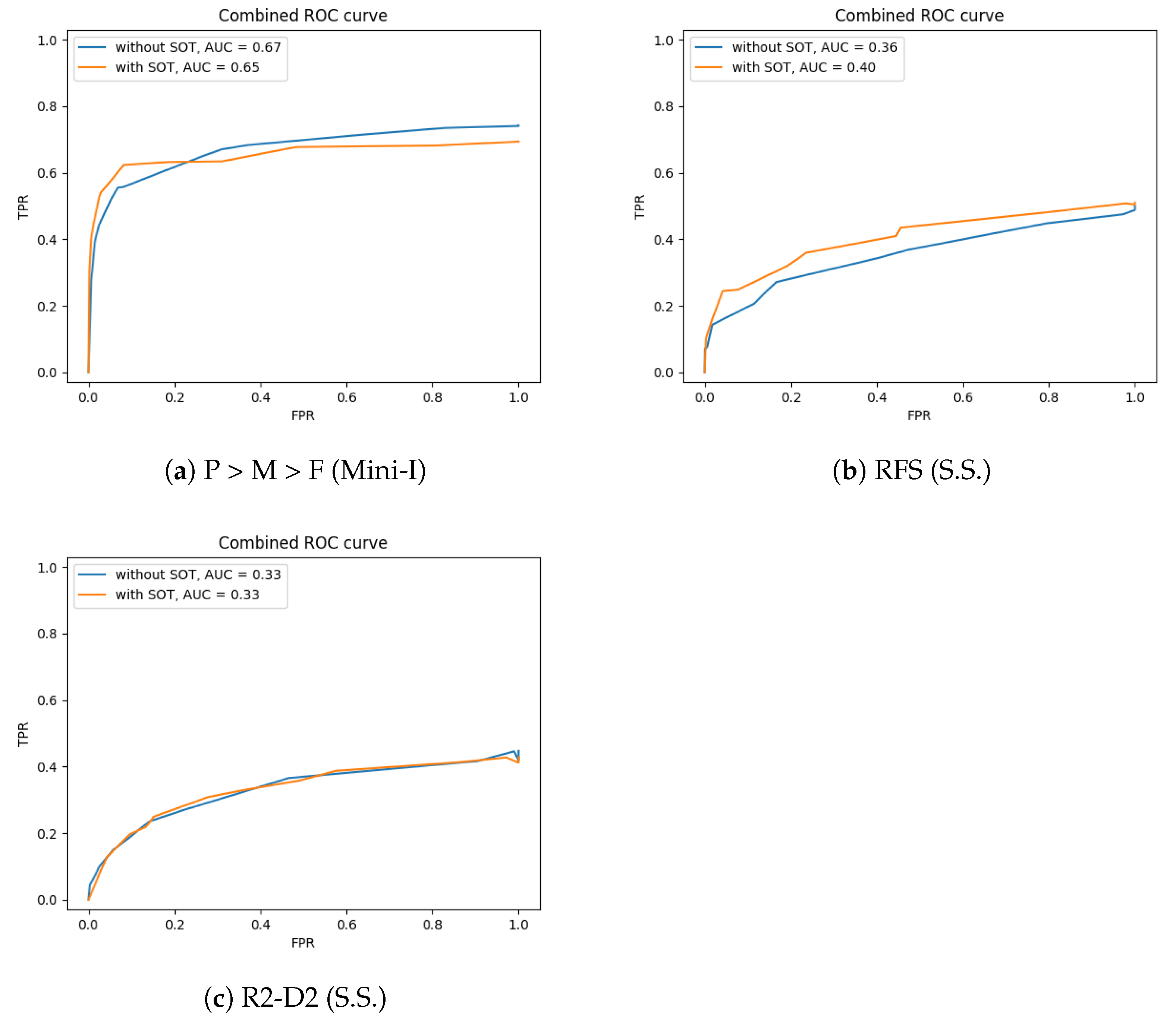
4.3.2. Additional Feature Transformation

Researchers in the FSL field have also investigated the effectiveness of additional feature transformation methods applied after a given feature extractor but before classification. SOT (self-optimal-transport) [43] is a parameterless (not learned) feature transformation that helps to cluster feature points in high-dimensional space; it has been shown by the authors to improve networks’ performance for both FSL and re-identification tasks.

To verify its effectiveness under our more realistic few-shot classification settings, we compare network performance with or without the SOT module. We conduct the same implementation test for the three representative networks (P > M > F (Mini-I), RFS (S.S.), R2-D2 (S.S.)), and the resulting comparisons are shown in Figure 7. For RFS, the SOT transformation indeed improved the matching results, although only by a small amount. The effect is not significant with R2-D2, and in the case of P > M > F it actually degrades the performance slightly.

Therefore, while this additional feature transformation consistently improves a network’s performance on the benchmark datasets [43], it does not necessarily improve the result in a more complex setting. The user may need to conduct additional evaluations before deciding whether to incorporate SOT or another feature transformation into the feature matching pipeline.

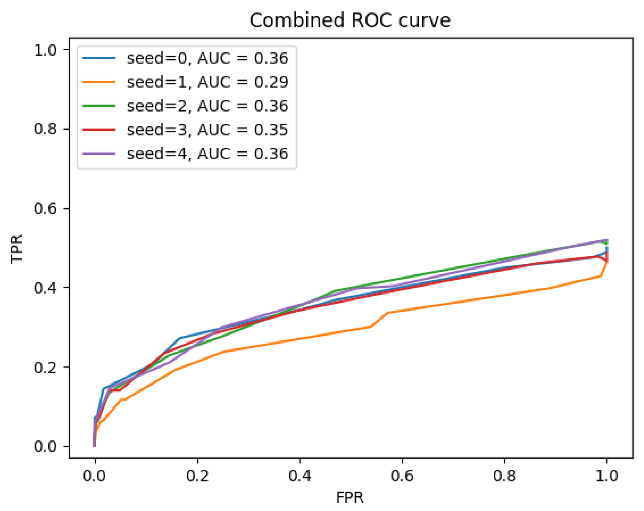
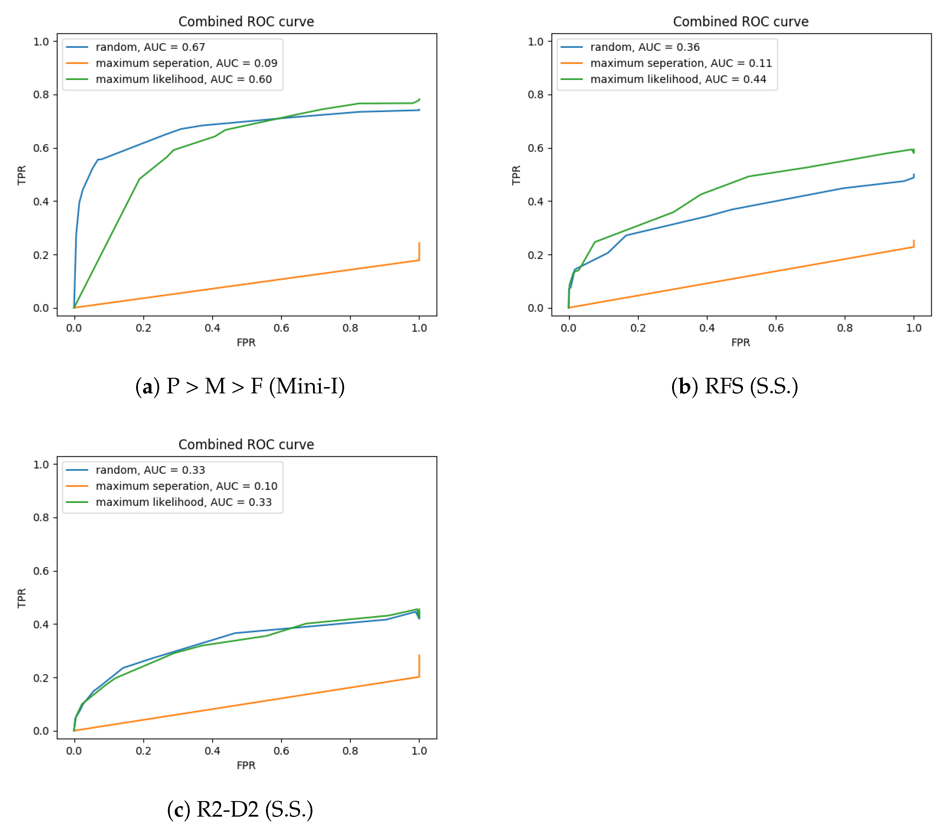
4.3.3. Support Data Selection

When we follow the FSL philosophy in a real-world implementation scenario, a few images per class need to be labeled to serve as the support set. Unknown images are then compared against the support set in order to be classified. Therefore, a question arises when we consider a real-world implementation scenario without a pre-defined dataset—which images should serve as the support set? Should we pick the most high-quality images, or should we pick the most diverse set?

As stated in Section 3.3.2, when conducting the implementation experiment, we first randomly select 10 images per class to serve as the support set. To verify that the selection of the support set does influence system performance, we repeat the experiment using different random seeds when selecting these 10 images. The results are shown in Figure 8. We can clearly see that the different random selections of the support images do affect performance; hence, we investigate next how strategies to choose the support images might help improve the performance.

From an intuitive standpoint, there are two potential selection strategies besides just random selection. The first method, named the “maximum separation” method, tries to find the most diverse set of images within that class. We implement this strategy by starting with one random image as an “anchor”, and then finding the next image whose feature is furthest from the initial anchor image’s feature. Subsequently, the third image should have the furthest average distance to the two previously enrolled images. We repeat the process until all ten images have been enrolled. The general idea of this selection scheme is to obtain the “most different-looking” images for a specific class.

The second method has the goal of finding the most common set of images within that class; we will call it the“maximum likelihood” method. For this method, we first apply PCA to reduce the feature dimension to a relatively small number D (D = 10 in this experiment) in order to reduce computational cost. We then assume the images follow a multivariate Gaussian distribution and compute the mean and covariance of the distribution. In this way, we compute a likelihood score for each image, and the ten images with the highest likelihood scores are selected. The general idea of this selection scheme is to obtain the “most common-looking” images for a specific class.

We also include the default random selection scheme as a reference point.

Next, we evaluate these two selection methods along with random selection by applying them using the three representative networks in implementation settings, namely, P > M > F (Mini-I), RFS (S.S.), and R2-D2 (S.S.). The results are shown in Figure 9. Overall, maximum separation is the worst and degrades the performance by a large margin. The maximum likelihood selection scheme shows noticeable improvements for RFS, but fails to show any significant advantage over random selection for the other two networks. Nevertheless, we believe the experiment demonstrates the necessity of considering which images should be selected to form the support set when dealing with raw data, and we encourage further investigation of this aspect.

4.3.4. Ease of Implementation

One final aspect to discuss is how easily a network can be modified and applied to a real-world system, particularly related to its flexibility when the task requirement changes. This issue arises when incorporating $e^{3}bm$ in our implementation settings. For every other network we considered in this paper, the feature extractor is trainable, and the decision making applies a deterministic feature comparison method such as closest match or k-nearest-neighbor. In contrast, $e^{3}bm$’s decision making involves a sophisticated ensemble of classifiers with trainable hyper-parameters, which poses major challenges when applying it to a different task than it was originally designed for.

To elaborate further, for the results presented in this paper, we have trained each network using “5-way 5-shot” settings, which is quite common in FSL benchmark protocols. However, during implementation on real data, we are interested in applying an 11-way classification problem, with the additional challenge of rejecting distractor images. For every other network, we can simply take the trained feature extractor and apply the feature comparison mechanism. However, for $e^{3}bm$, its sophisticated ensemble of classifiers is constrained to perform a 5-way classification problem. As a result, when we take out the feature extractor and apply a deterministic classifier, the trained parameters and hyper-parameters associated with the complex classifier are lost. That is one reason why $e^{3}bm$ performs poorly in the implementation setting.

It is clear that few-shot learning was proposed to help practitioners adapt to new tasks quickly with minimum labeling efforts. Therefore, we believe networks designed for FSL should accommodate not only a domain shift (e.g., the change from one 5-way classification problem to another 5-way classification problem in a new environment), but also to reasonable changes in the classification problem itself (e.g., the change from a 5-way classification problem to a 6-way classification problem). Therefore, we encourage researchers in the FSL field to remember the end goal, rather than striving solely to optimize network performance on a benchmark dataset.

5. Conclusions

The main focus of this paper has been to bridge the gap between the study of few-shot learning (FSL) and the deployment of FSL classifiers for real-world problems. Here, we explore a practical problem—animal species classification for in-the-wild camera-trap images—as the example for a realistic FSL application, where FSL should alleviate the major difficulty of not having labels for a new environment. This puts the theory of FSL to the test since our real-world problem has additional challenges, including lower image quality, the presence of distractors, and unbalanced class distributions. These additional challenges caused by real-world data were described in Section 3.1.

To understand the performance of each FSL network for this problem, we create two datasets from our data: (1) a benchmark-style dataset that enables an exploration into a network’s effectiveness under a new environment and a new task, and (2) an implementation-style dataset that focuses on a network’s effectiveness under additional challenges such as the presence of distractors and imbalanced class distributions. The implementation-style dataset also introduces new experiments and several additional performance metrics. We describe the construction of the datasets and evaluation protocols in Section 3.3. We then conduct experiments and report results using these two testing datasets. Specifically, in Section 4.1, we report the detailed testing results for both our datasets, and observe many cases that indicate that performance benchmark datasets do not necessarily reflect a network’s true usefulness in real-world scenarios. In Section 4.2, we discuss the benefit of having external training data and how that affects a network’s performance in real-world settings. Finally, in Section 4.3, we perform additional experiments exclusively within the implementation settings, to explore how various factors influence a network’s effectiveness in real-world settings. These factors include both network design choices as well as things such as support set selection, which were not considered when a benchmark dataset is in place.

We believe there is more work to be done. There exist many other factors that may affect a network’s real-world performance but have not been incorporated into benchmark testing. For example, there is more to understand about how to create an effective training set from public data for training an FSL network for a given domain. We also encourage researchers in the FSL area to stay true to the origin of the problem. There is an increasing tendency to focus primarily on obtaining high accuracy on benchmark datasets, but FSL was proposed to make systems easily adaptable to new environments and tasks. We encourage additional renewed effort to this original goal.

References

1. Li, F.-F.; Fergus, R.; Perona, P. One-shot learning of object categories. IEEE Trans. Pattern Anal. Mach. Intell. 2006, 28, 594–611. [Google Scholar] [CrossRef] [PubMed] [Green Version]
2. Vinyals, O.; Blundell, C.; Lillicrap, T.; Kavukcuoglu, K.; Wierstra, D. Matching networks for one shot learning. In Proceedings of the 30th International Conference on Neural Information Processing Systems, Barcelona, Spain, 5–10 December 2016. [Google Scholar]
3. Wang, Y.; Yao, Q.; Kwok, J.T.; Ni, L.M. Generalizing from a few examples: A survey on few-shot learning. ACM Comput. Surv. 2020, 53, 1–34. [Google Scholar] [CrossRef]
4. Chen, H.; Lindshield, S.M.; Reibman, A.R. Challenges and constraints when applying few shot learning to a real-world scenario: In-the-wild camera-trap species classification. Electron. Imaging 2023, 35, 280-1–280-6. [Google Scholar] [CrossRef]
5. Lindshield, S.; Bogart, S.; Gueye, M.; Ndiaye, P.; Pruetz, J. Informing Protection Efforts for Critically Endangered Chimpanzees (Pan troglodytes verus) and Sympatric Mammals amidst Rapid Growth of Extractive Industries in Senegal. Folia Primatol. 2019, 90, 124–136. [Google Scholar] [CrossRef] [PubMed]
6. Pruetz, J.; Bertolani, P.; Boyer Ontl, K.; Lindshield, S.; Shelley, M.; Wessling, E. New evidence on the tool-assisted hunting exhibited by chimpanzees (Pan troglodytes verus) in a savannah habitat at Fongoli, Sénégal. R. Soc. Open Sci. 2015, 2, 140507. [Google Scholar] [CrossRef] [Green Version]
7. Norouzzadeh, M.S.; Nguyen, A.; Kosmala, M.; Swanson, A.; Palmer, M.S.; Packer, C.; Clune, J. Automatically identifying, counting, and describing wild animals in camera-trap images with deep learning. Proc. Natl. Acad. Sci. USA 2018, 115, E5716–E5725. [Google Scholar] [CrossRef] [Green Version]
8. Pavlovs, I.; Aktas, K.; Avots, E.; Vecvanags, A.; Filipovs, J.; Brauns, A.; Done, G.; Jakovels, D.; Anbarjafari, G. Ungulate Detection and Species Classification from Camera Trap Images Using RetinaNet and Faster R-CNN. Entropy 2022, 24, 353. [Google Scholar] [CrossRef]
9. Zhang, Z.; He, Z.; Cao, G.; Cao, W. Animal Detection From Highly Cluttered Natural Scenes Using Spatiotemporal Object Region Proposals and Patch Verification. IEEE Trans. Multimed. 2016, 18, 2079–2092. [Google Scholar] [CrossRef]
10. Singh, P.; Lindshield, S.M.; Zhu, F.; Reibman, A.R. Animal Localization in Camera-Trap Images with Complex Backgrounds. In Proceedings of the IEEE Southwest Symposium on Image Analysis and Interpretation (SSIAI), Albuquerque, NM, USA, 29–31 March 2020; pp. 66–69. [Google Scholar] [CrossRef]
11. Karami, A.; Crawford, M.; Delp, E.J. Automatic Plant Counting and Location Based on a Few-Shot Learning Technique. IEEE J. Sel. Top. Appl. Earth Obs. Remote Sens. 2020, 13, 5872–5886. [Google Scholar] [CrossRef]
12. Tian, Z.; Lai, X.; Jiang, L.; Liu, S.; Shu, M.; Zhao, H.; Jia, J. Generalized Few-shot Semantic Segmentation. In Proceedings of the IEEE/CVF Conference on Computer Vision and Pattern Recognition, New Orleans, LA, USA, 18–24 June 2022; pp. 11553–11562. [Google Scholar] [CrossRef]
13. Snell, J.; Swersky, K.; Zemel, R. Prototypical networks for few-shot learning. Adv. Neural Inf. Process. Syst. 2017, 30, 1–11. [Google Scholar]
14. Tian, Y.; Wang, Y.; Krishnan, D.; Tenenbaum, J.B.; Isola, P. Rethinking few-shot image classification: A good embedding is all you need? In Proceedings of the European Conference on Computer Vision (ECCV), Glasgow, UK, 23–28 August 2020; pp. 266–282. [Google Scholar] [CrossRef]
15. Chen, W.Y.; Liu, Y.C.; Kira, Z.; Wang, Y.C.; Huang, J.B. A Closer Look at Few-shot Classification. In Proceedings of the International Conference on Learning Representations (ICLR), New Orleans, LA, USA, 6–9 May 2019. [Google Scholar]
16. Finn, C.; Abbeel, P.; Levine, S. Model-agnostic meta-learning for fast adaptation of deep networks. In Proceedings of the International Conference on Machine Learning, Sydney, NSW, Australia, 6–11 August 2017; pp. 1126–1135. [Google Scholar]
17. Liu, Y.; Schiele, B.; Sun, Q. An Ensemble of Epoch-wise Empirical Bayes for Few-shot Learning. In Proceedings of the European Conference on Computer Vision (ECCV), Glasgow, UK, 23–28 August 2020. [Google Scholar] [CrossRef]
18. Xiong, C.; Li, W.; Liu, Y.; Wang, M. Multi-Dimensional Edge Features Graph Neural Network on Few-Shot Image Classification. IEEE Signal Process. Lett. 2021, 28, 573–577. [Google Scholar] [CrossRef]
19. Jiang, B.; Zhao, K.; Tang, J. RGTransformer: Region-Graph Transformer for Image Representation and Few-Shot Classification. IEEE Signal Process. Lett. 2022, 29, 792–796. [Google Scholar] [CrossRef]
20. Lake, B.M.; Salakhutdinov, R.; Tenenbaum, J.B. Human-level concept learning through probabilistic program induction. Science 2015, 350, 1332–1338. [Google Scholar] [CrossRef] [Green Version]
21. Sun, Q.; Liu, Y.; Chua, T.; Schiele, B. Meta-Transfer Learning for Few-Shot Learning. In Proceedings of the IEEE/CVF Conference on Computer Vision and Pattern Recognition, Long Beach, CA, USA, 15–20 June 2019; pp. 403–412. [Google Scholar] [CrossRef] [Green Version]
22. Bennequin, E.; Tami, M.; Toubhans, A.; Hudelot, C. Few-Shot Image Classification Benchmarks are Too Far From Reality: Build Back Better with Semantic Task Sampling. In Proceedings of the IEEE/CVF Conference on Computer Vision and Pattern Recognition Workshops, New Orleans, LA, USA, 19–20 June 2022; pp. 4766–4775. [Google Scholar] [CrossRef]
23. Ravi, S.; Larochelle, H. Optimization as a model for few-shot learning. In Proceedings of the International Conference on Learning Representations (ICLR), Toulon, France, 24–26 April 2017. [Google Scholar]
24. Wah, C.; Branson, S.; Welinder, P.; Perona, P.; Belongie, S. Caltech-UCSD Birds 200; Technical Report CNS-TR-2011-001; California Institute of Technology: Pasadena, CA, USA, 2011. [Google Scholar]
25. Nuthalapati, S.; Tunga, A. Multi-Domain Few-Shot Learning and Dataset for Agricultural Applications. In Proceedings of the IEEE/CVF International Conference on Computer Vision Workshops (ICCVW), Montreal, BC, Canada, 11–17 October 2021; pp. 1399–1408. [Google Scholar] [CrossRef]
26. Zhang, A.; Li, S.; Cui, Y.; Yang, W.; Dong, R.; Hu, J. Limited Data Rolling Bearing Fault Diagnosis With Few-Shot Learning. IEEE Access 2019, 7, 110895–110904. [Google Scholar] [CrossRef]
27. Yoo, T.K.; Choi, J.Y.; Kim, H.K. Feasibility study to improve deep learning in OCT diagnosis of rare retinal diseases with few-shot classification. Med. Biol. Eng. Comput. 2021, 59, 401–415. [Google Scholar] [CrossRef] [PubMed]
28. Koch, G.; Zemel, R.; Salakhutdinov, R. Siamese neural networks for one-shot image recognition. In Proceedings of the ICML Deep Learning Workshop, Lille, France, 6–11 July 2015; Volume 2. [Google Scholar]
29. Figueroa-Mata, G.; Mata-Montero, E. Using a Convolutional Siamese Network for Image-Based Plant Species Identification with Small Datasets. Biomimetics 2020, 5, 8. [Google Scholar] [CrossRef] [Green Version]
30. Zhu, J.Y.; Park, T.; Isola, P.; Efros, A.A. Unpaired Image-to-Image Translation Using Cycle-Consistent Adversarial Networks. In Proceedings of the IEEE International Conference on Computer Vision (ICCV), Venice, Italy, 22–29 October 2017; pp. 2242–2251. [Google Scholar] [CrossRef] [Green Version]
31. Prabhu, V.; Kannan, A.; Ravuri, M.; Chablani, M.; Sontag, D.A.; Amatriain, X. Prototypical Clustering Networks for Dermatological Disease Diagnosis. arXiv 2018, arXiv:1811.03066. [Google Scholar]
32. Wang, L.; Yang, X.; Tan, H.; Bai, X.; Zhou, F. Few-Shot Class-Incremental SAR Target Recognition Based on Hierarchical Embedding and Incremental Evolutionary Network. IEEE Trans. Geosci. Remote Sens. 2023, 61, 5204111. [Google Scholar] [CrossRef]
33. Zhong, Q.; Chen, L.; Qian, Y. Few-Shot Learning for Remote Sensing Image Retrieval with MAML. In Proceedings of the IEEE International Conference on Image Processing (ICIP), Abu Dhabi, United Arab Emirates, 25–28 October 2020; pp. 2446–2450. [Google Scholar] [CrossRef]
34. Bertinetto, L.; Henriques, J.F.; Torr, P.H.S.; Vedaldi, A. Meta-learning with differentiable closed-form solvers. In Proceedings of the International Conference on Learning Representations (ICLR), New Orleans, LA, USA, 6–9 May 2019. [Google Scholar]
35. Kang, D.; Kwon, H.; Min, J.; Cho, M. Relational Embedding for Few-Shot Classification. In Proceedings of the IEEE/CVF International Conference on Computer Vision (ICCV), Montreal, QC, Canada, 10–17 October 2021. [Google Scholar]
36. Chen, D.; Chen, Y.; Li, Y.; Mao, F.; He, Y.; Xue, H. Self-Supervised Learning for Few-Shot Image Classification. In Proceedings of the IEEE International Conference on Acoustics, Speech and Signal Processing (ICASSP), Toronto, ON, Canada, 6–11 June 2021; pp. 1745–1749. [Google Scholar] [CrossRef]
37. Hu, S.X.; Li, D.; Stühmer, J.; Kim, M.; Hospedales, T.M. Pushing the Limits of Simple Pipelines for Few-Shot Learning: External Data and Fine-Tuning Make a Difference. In Proceedings of the IEEE/CVF Conference on Computer Vision and Pattern Recognition, New Orleans, LA, USA, 18–24 June 2022. [Google Scholar] [CrossRef]
38. Swanson, A.; Kosmala, M.; Lintott, C.; Simpson, R.; Smith, A.; Packer, C. Snapshot Serengeti, high-frequency annotated camera trap images of 40 mammalian species in an African savanna. Sci. Data 2015, 2, 150026. [Google Scholar] [CrossRef] [Green Version]
39. Caron, M.; Touvron, H.; Misra, I.; Jégou, H.; Mairal, J.; Bojanowski, P.; Joulin, A. Emerging properties in self-supervised vision transformers. In Proceedings of the IEEE/CVF International Conference on Computer Vision (ICCV), Montreal, QC, Canada, 10–17 October 2021; pp. 9650–9660. [Google Scholar] [CrossRef]
40. He, K.; Zhang, X.; Ren, S.; Sun, J. Deep Residual Learning for Image Recognition. In Proceedings of the IEEE/CVF Conference on Computer Vision and Pattern Recognition, Las Vegas, NV, USA, 27–30 June 2016; pp. 770–778. [Google Scholar] [CrossRef] [Green Version]
41. Zagoruyko, S.; Komodakis, N. Wide residual networks. arXiv 2016, arXiv:1605.07146. [Google Scholar]
42. Bachman, P.; Hjelm, R.D.; Buchwalter, W. Learning representations by maximizing mutual information across views. In Proceedings of the 33rd Conference on Neural Information Processing Systems (NeurIPS 2019), Vancouver, BC, Canada, 8–14 December 2019. [Google Scholar]
43. Shalam, D.; Korman, S. The Self-Optimal-Transport Feature Transform. arXiv 2022, arXiv:2204.03065. [Google Scholar]
Figure 1. Hard-to-distinguish species with similar build and color.
Ai 04 00031 g001
Figure 2. Hard-to-distinguish species due to similar background.
Ai 04 00031 g002
Figure 3. Hard-to-distinguish species due to similar build and low image quality.
Ai 04 00031 g003
Figure 4. Number of bounding boxes for each species.
Ai 04 00031 g004
Figure 5. Best ROC curves for each network when testing on Senegal-I. The datasets used for training (e.g., mini-ImageNet or Snapshot Serengeti) are included in parentheses. Full results are shown in the Appendix A, Figure A1.
Ai 04 00031 g005
Figure 6. ROC curves for using pre-trained backbone only and P > M > F further trained on mini-ImageNet/Snapshot Serengeti. Testing is on Senegal-I.
Ai 04 00031 g006
Figure 7. Effect of self-optimal-transport.
Ai 04 00031 g007
Figure 8. Different random selections of support images, using RFS trained on S.S.
Ai 04 00031 g008
Figure 9. Effect of three selection schemes for selecting the support set.
Ai 04 00031 g009