

Improving Alzheimer’s Disease and Brain Tumor Detection Using Deep Learning with Particle Swarm Optimization


Abstract
:1. Introduction
- We develop a hybrid framework that employs the PSO algorithm to determine the best hyper-parameters’ configuration for CNN architectures to improve prediction accuracy for brain diseases and decrease the loss function value.
- We utilize PSO as a wrapper around the training process to retrieve hyper-parameters (such as the number of convolution filters, the size of the filters used in the convolutional layer, the size of the pool in the max pooling layer, and the size of the strides used in the max pooling layer).
- We contrast our PSO-optimized CNN model with three distinct CNN models: the ResNet, the InceptionNet, and the VGG models. Finally, we benchmarked our proposed model against state-of-the-art models employing different optimization algorithms.
2. Related Work

| Reference | Dataset Type | Proposed Model | Study Limitation | Evaluation Results |
|---|---|---|---|---|
| [18] | AD Dataset | 3D CNN (VoxCNN, ResNet), Softmax | Small dataset size, model complexity, lack of interpretability and external validation | AD vs. NC Accuracy: 79% VoxCNN Accuracy: 80% ResNet AUC: 88% VoxCNN AUC: 87% ResNet |
| [19] | AD Dataset | CNN, SVM | Lack of implementation, training, and parameter details | AD vs. NC Accuracy: 96% |
| [20] | AD Dataset | CNN (AlexNet), SVM | Insufficient discussion on feature selection and extraction from MRI data | AD vs. NC Accuracy: 90% Specificity: 91% Sensitivity: 87% |
| [21] | AD Dataset | FreeSurfer, SVM, Naive Bayesian, Random Forest, Decision Tree | Limitations in choice of evaluation metrics | AD vs. NC Accuracy: 75% Specificity: 77% Sensitivity: 75% F-score: 72% AUC: 76% |
| [22] | AD Dataset | PSO-based PIDC algorithm, Softmax | Lack of extensive details and evaluation of the hybrid algorithm for brain image segmentation | AD vs. NC Accuracy: 92% |
| [23] | AD Dataset | PSO with Decision Tree Methods | Insufficient analysis or discussion of feature selection process | AD vs. NC Accuracy: 93.56% |
| [24] | AD Dataset | GA algorithm, ELM, PSO | Lack of thorough comparison with other classifiers or methods | AD vs. NC Accuracy: 87.23% |
| [25] | Brain Tumor Dataset | CNN, Softmax | Insufficient details or analysis of CNN architecture for brain tumor classification | Normal vs. Not Normal Accuracy: 94.39% |
| [26] | Brain Tumor Dataset | GA algorithm, SVM | Lack of extensive details or analysis of optimization technique for brain tumor detection | Normal vs. Not Normal Accuracy: 91% |
| [27] | Brain Tumor Dataset | CNN, ELM, SVM | Insufficient details or analysis of ensemble classifier for brain tumor segmentation and classification | Normal vs. Not Normal Accuracy: 91.17% |
| [29] | Brain Tumor Dataset | CNN (VGG19), Softmax | Lack of details or analysis of deep CNN architecture and hyper-parameters for brain tumor classification | Normal vs. Not Normal Accuracy: 90.67% |
| [31] | Brain Tumor Dataset | CNN with DWT, SVM | Lack of details or analysis of PSO-based segmentation technique for brain MRI images and comparison with other methods | Normal vs. Not Normal Accuracy: 85% |
| [32] | Brain Tumor Dataset | CNN with PSO, Softmax | Lack of details or analysis of modified PSO algorithm for brain tumor detection and limitations of the modification | Normal vs. Not Normal Accuracy: 92% |
| Reference | Usage of PSO |
|---|---|
| [18] | Not used PSO |
| [19] | Not Used PSO |
| [20] | Not Used PSO |
| [21] | Not Used PSO |
| [22] | PSO was used for optimizing the model performance by selecting the optimal parameters and weight |
| [23] | PSO was used for the feature selection process |
| [24] | PSO was used for optimizing the model performance by selecting the optimal parameters and weight |
| [25] | Not used PSO |
| [26] | Not used PSO |
| [27] | Not used PSO |
| [29] | Not used PSO |
| [31] | PSO was used for the feature selection process |
| [32] | PSO was used for the feature selection process |
3. Proposed Methodology
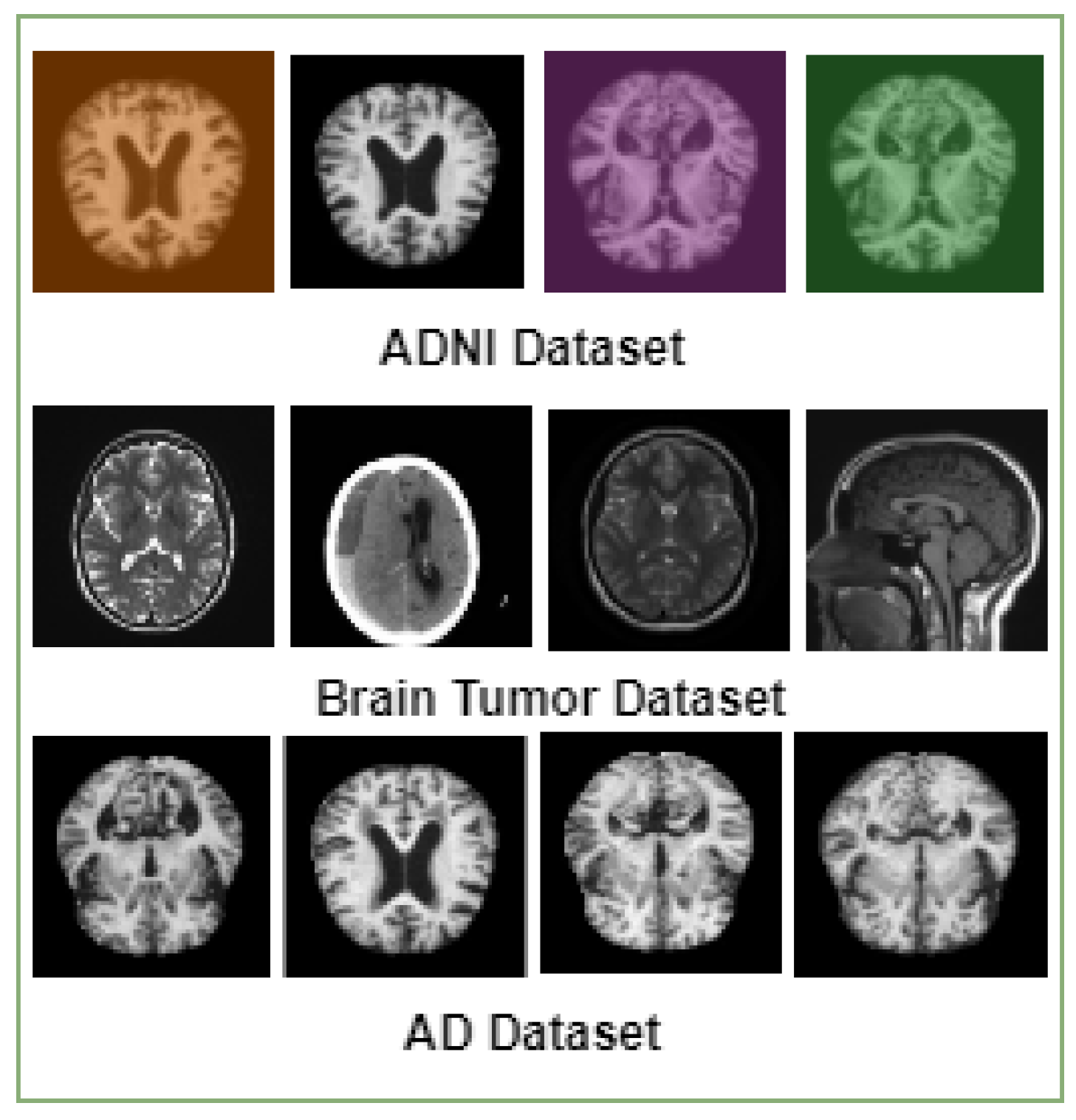
3.1. MRI Datasets
3.2. Data Pre-Processing
3.3. Proposed Detection Framework
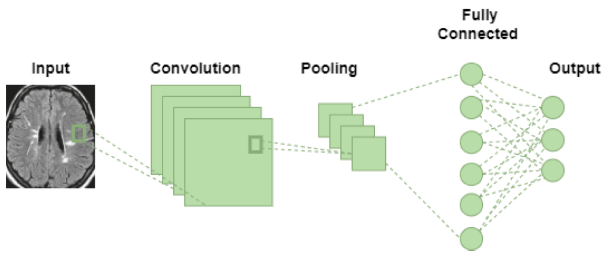
3.3.1. Convolutional Neural Network (CNN)
3.3.2. Particle Swarm Optimization (PSO)
| Algorithm 1: Particle Swarm Optimization (PSO) Algorithm | |||||||
| Require: Objective function | |||||||
| Require: Hyperparameters n, Fitness function F | |||||||
| Ensure: Optimal solution | |||||||
 | |||||||
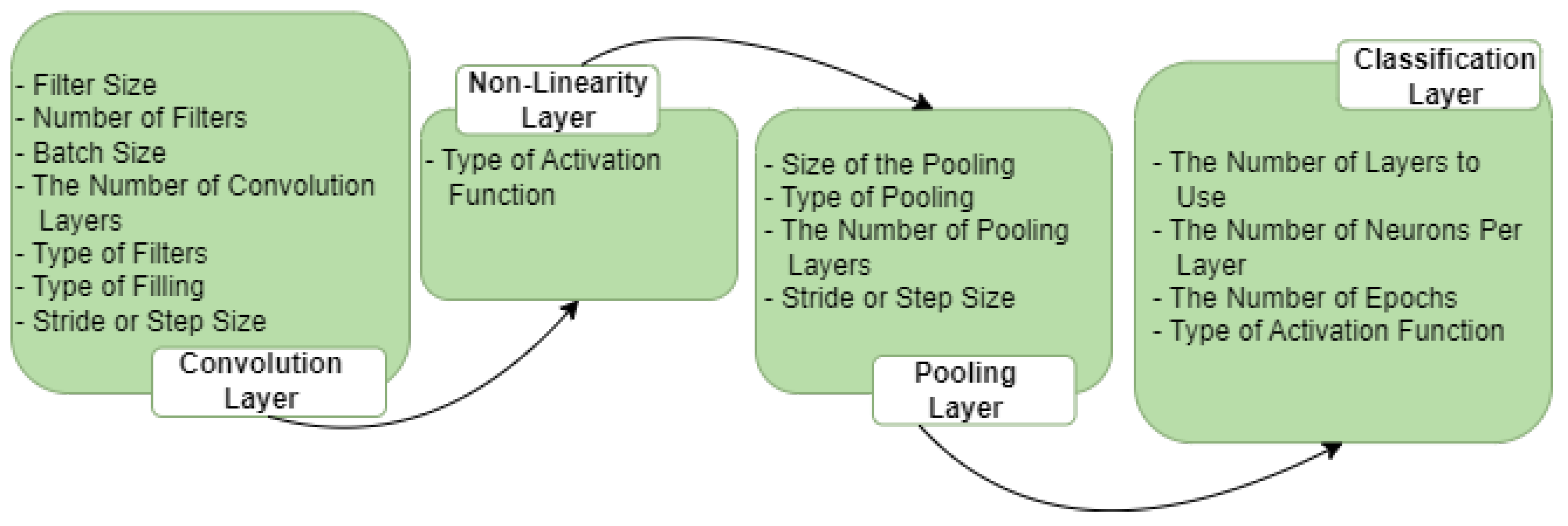
3.3.3. Optimal Selection of Hyper-Parameters via PSO Algorithm
- The number of filters in convolutional layers.
- The size of filters in convolutional layers.
- The size of the pool in the max pooling layer.
- The size of the strides used in the max pooling layer.
- 1.
- Initialization of the SwarmIn the swarm, each particle’s initial position in the n-dimensional space is randomly selected from a uniform distribution U(, ), where and represent the lower and upper limits. The particle’s position is then designated as its best-known position, denoted by . If the fitness value exceeds the fitness value of the swarm’s best global position, , is stored as the new best position in the swarm, referred to as . The particle’s velocity is randomly determined from a uniform distribution, considering the constraints of the hyper-parameter limits. Following the initialization, the swarm, consisting of s particles represented as tuples for , undergoes evolutionary processes.
- 2.
- Evaluation of the SwarmIn each generation of a swarm (referred to as gen, where represents the maximum number of generations), the velocity values of all particles are updated using the following equation:Here, and are randomly drawn from a uniform distribution to add a stochastic element to the velocity updates, enhancing search space exploration. The inertia weight scales the velocity, while and are acceleration coefficients that determine the influence of the best particle position () and the best swarm position () on the velocity changes. Subsequently, the particle’s position is updated accordingly.Following this, the best position for each particle and the best swarm position are modified. These updates are only applied if there has been a change. The evolutionary process continues until one of the following termination conditions is met:
- (a)
- The best position in the swarm () has been displaced by an amount smaller than a specified minimum step size denoted as .
- (b)
- The fitness value of the best particle has improved by an amount less than a predefined threshold denoted by .
- (c)
- The maximum number of swarm generations, , has been reached.
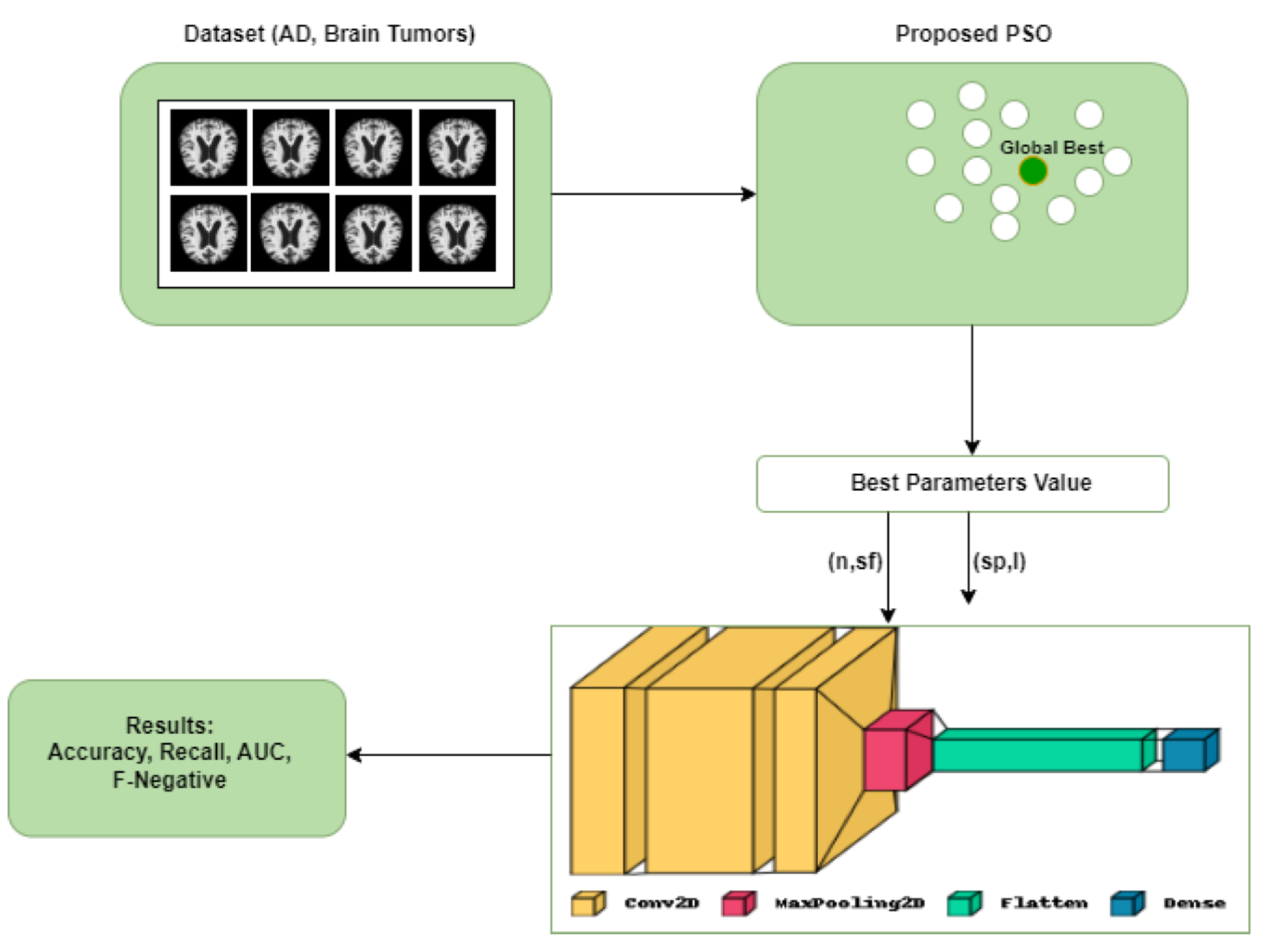
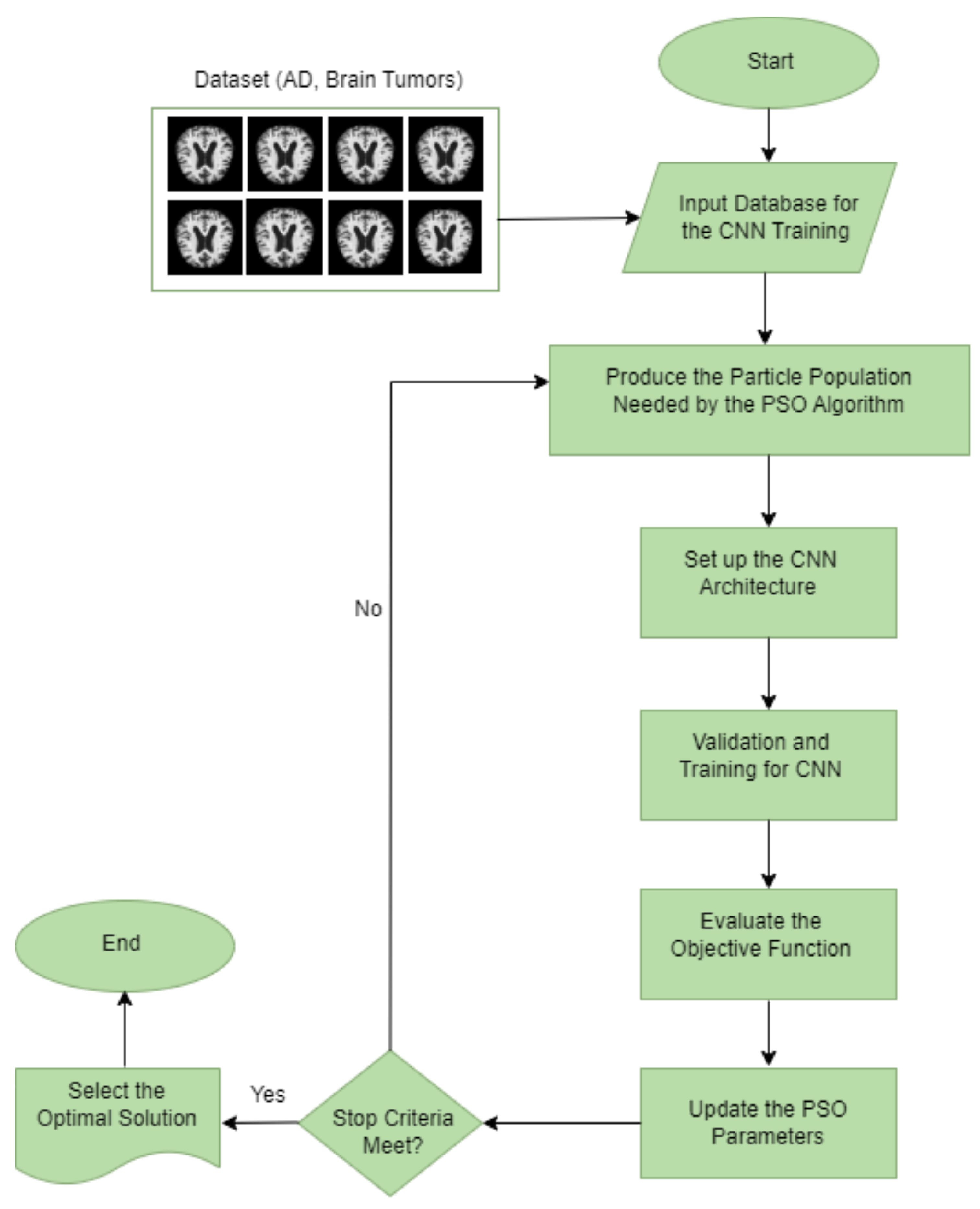
The first termination condition is designed to prevent high-quality oscillation between two neighboring solutions. The second condition is satisfied when the swarm optimization converges to a well-fitted particle unlikely to improve further. Finally, the best position in the swarm () is returned as the output.The efficiency of PSO is influenced by the number of hyper-parameters involved, and this can be denoted aswhere s and are constants, the time complexity primarily stems from the evaluation of , which scales linearly with the parameter n.Figure 4 illustrates the whole architecture of our methodology used in this study. The CNN initially uses the PSO algorithm for parameter optimization. The PSO is initialized in this process by the execution parameters, and this generates the particles. Each solution represents a completed CNN training period because each particle is a possible solution, and its position has a parameter that needs to be used in the proposed CNN architecture. Our CNN architecture is designed with a concise yet flexible structure. It comprises a block comprising convolutional and max pooling layers, followed by a Softmax activation function for classification. Table 3 and Table 4 list the convolutional and maximum pooling layer parameters and the permitted ranges for each.
- 1.
- Input database for the CNN training: this step chooses the database that will be processed and classified for CNN. It is important to note that each database’s components must maintain a consistent structure or set of attributes with the same pixel size and file format.
- 2.
- Produce the particle population needed by the PSO algorithm: the PSO parameters were set to include the experiment’s number of iterations, particle numbers, inertial weight, cognitive constant (C1), and social constant (C2). Table 4 lists the PSO parameters used in the experiment.
- 3.
- Set up the CNN architecture: create the CNN architecture using the PSO parameter (the number of filters and the size of the filters in the convolution layers, the size of the pool in the max pooling layer, and the size of the strides in the max pooling layer), along with the additional parameters listed in Table 4.
- 4.
- Validation and training for CNN: after reading and processing the input databases and collecting the images for training, validation, and testing, the CNN generates a recognition rate in this step. The objective function’s return value includes these values for the PSO.
- 5.
- Determine the objective function: the PSO algorithm evaluates the objective function defined in Equation (1) to select the best parameters.
- 6.
- Update the PSO parameters: each particle adjusts its velocity and location at each iteration based on its best position (Pbest) in the search space and the best position for the entire swarm (Gbest).
- 7.
- Repeat the process: the number of iterations is the stopping criterion in our study, which involves evaluating all the particles until the stopping criteria are satisfied.
- 8.
- Select the optimal solution: the particle Gbest represents the best solution in this process for the CNN model.
4. Experiments and Results
4.1. Optimization Results Obtained by the PSO-CNN Method
4.2. Comparison with Existing Transfer Learning Model
4.3. Comparison with Existing Transfer Learning Model
5. Conclusions and Future Work
Author Contributions
Funding
Institutional Review Board Statement
Informed Consent Statement
Data Availability Statement
Conflicts of Interest
References
- Anton, A.; Fallon, M.; Cots, F.; Sebastian, M.A.; Morilla-Grasa, A.; Mojal, S.; Castells, X. Cost and detection rate of glaucoma screening with imaging devices in a primary care center. Clin. Ophthalmol. 2017, 16, 337–346. [Google Scholar] [CrossRef] [PubMed] [Green Version]
- Alzheimer’s Disease International. World Alzheimer Report 2018. The State of the Art of Dementia Research: New Frontiers; Alzheimer’s Disease International (ADI): London, UK, 2018; pp. 14–20. [Google Scholar]
- Huang, J.; van Zijl, P.C.; Han, X.; Dong, C.M.; Cheng, G.W.; Tse, K.H.; Knutsson, L.; Chen, L.; Lai, J.H.; Wu, E.X.; et al. Altered d-glucose in brain parenchyma and cerebrospinal fluid of early Alzheimer’s disease detected by dynamic glucose-enhanced MRI. Sci. Adv. 2020, 6, eaba3884. [Google Scholar] [CrossRef] [PubMed]
- Castellazzi, G.; Cuzzoni, M.G.; Cotta Ramusino, M.; Martinelli, D.; Denaro, F.; Ricciardi, A.; Vitali, P.; Anzalone, N.; Bernini, S.; Palesi, F.; et al. A machine learning approach for the differential diagnosis of alzheimer and vascular dementia fed by MRI selected features. Front. Neuroinform. 2020, 14, 25. [Google Scholar] [CrossRef] [PubMed]
- Zaw, H.T.; Maneerat, N.; Win, K.Y. Brain tumor detection based on Naïve Bayes Classification. In Proceedings of the 2019 5th International Conference on Engineering, Applied Sciences and Technology (ICEAST), Luang Prabang, Laos, 2–5 July 2019; pp. 1–4. [Google Scholar]
- Ghnemat, R.; Khalil, A.; Al-Haija, Q.A. Ischemic stroke lesion segmentation using mutation model and generative adversarial network. Electronics 2023, 12, 590. [Google Scholar] [CrossRef]
- Salam, A.A.; Khalil, T.; Akram, M.U.; Jameel, A.; Basit, I. Automated detection of glaucoma using structural and non structural features. Springerplus 2016, 5, 1–21. [Google Scholar] [CrossRef] [PubMed] [Green Version]
- Yadav, A.S.; Kumar, S.; Karetla, G.R.; Cotrina-Aliaga, J.C.; Arias-Gonzáles, J.L.; Kumar, V.; Srivastava, S.; Gupta, R.; Ibrahim, S.; Paul, R.; et al. A feature extraction using probabilistic neural network and BTFSC-net model with deep learning for brain tumor classification. J. Imaging 2022, 9, 10. [Google Scholar] [CrossRef] [PubMed]
- Korolev, S.; Safiullin, A.; Belyaev, M.; Dodonova, Y. Residual and plain convolutional neural networks for 3D brain MRI classification. In Proceedings of the 2017 IEEE 14th international symposium on biomedical imaging (ISBI 2017), Melbourne, Australia, 18–21 April 2017; pp. 835–838. [Google Scholar]
- Hemanth, D.J.; Deperlioglu, O.; Kose, U. An enhanced diabetic retinopathy detection and classification approach using deep convolutional neural network. Neural Comput. Appl. 2020, 32, 707–721. [Google Scholar] [CrossRef]
- Wang, W.; Gang, J. Application of convolutional neural network in natural language processing. In Proceedings of the 2018 International Conference on Information Systems and Computer Aided Education (ICISCAE), Changchun, China, 6–8 July 2018; pp. 64–70. [Google Scholar]
- Al-Haija, Q.A.; Adebanjo, A. Breast Cancer Diagnosis in Histopathological Images Using ResNet-50 Convolutional Neural Network. In Proceedings of the 2020 IEEE International IOT, Electronics and Mechatronics Conference (IEMTRONICS 2020), Vancouver, BC, Canada, 9–12 September 2020. [Google Scholar]
- Al-Haija, Q.A.; Smadi, M.; Al-Bataineh, O.M. Identifying Phasic dopamine releases using DarkNet-19 Convolutional Neural Network. In Proceedings of the 2021 IEEE International IOT, Electronics and Mechatronics Conference (IEMTRONICS 2021), Toronto, ON, Canada, 21–24 April 2021; p. 590. [Google Scholar]
- Liang, S.D. Optimization for deep convolutional neural networks: How slim can it go? IEEE Trans. Emerg. Top. Comput. Intell. 2018, 4, 171–179. [Google Scholar] [CrossRef]
- Ma, B.; Li, X.; Xia, Y.; Zhang, Y. Autonomous deep learning: A genetic DCNN designer for image classification. Neurocomputing 2020, 379, 152–161. [Google Scholar] [CrossRef] [Green Version]
- Snoek, J.; Larochelle, H.; Adams, R.P. Practical Bayesian optimization of machine learning algorithms. Adv. Neural Inf. Process. Syst. 2012, 25, 1–9. [Google Scholar]
- Hutter, F.; Hoos, H.H.; Leyton-Brown, K. Sequential model-based optimization for general algorithm configuration. In Proceedings of the Learning and Intelligent Optimization: 5th International Conference, LION 5, Rome, Italy, 17–21 January 2011; Selected Papers 5. Springer: Berlin/Heidelberg, Germany, 2011; pp. 507–523. [Google Scholar]
- Poma, Y.; Melin, P.; González, C.I.; Martínez, G.E. Optimization of convolutional neural networks using the fuzzy gravitational search algorithm. J. Autom. Mob. Robot. Intell. Syst. 2020, 14, 109–120. [Google Scholar] [CrossRef]
- Anima890. Alzheimer’s Disease Classification Dataset. Kaggle. 2019. Available online via: https://www.kaggle.com/datasets/tourist55/alzheimers-dataset-4-class-of-images (accessed on 22 March 2023).
- Alzheimer’s Disease Neuroimaging Initiative. ADNI (Alzheimer’s Disease Neuroimaging Initiative). Available online: https://adni.loni.usc.edu/ (accessed on 11 May 2023).
- Nickparvar, M. Brain Tumor MRI Dataset. Available online: https://www.kaggle.com/datasets/masoudnickparvar/brain-tumor-mri-dataset (accessed on 11 May 2021).
- Al-Haija, Q.A.; Smadi, M.; Al-Bataineh, O.M. Early Stage Diabetes Risk Prediction via Machine Learning. In Proceedings of the 13th International Conference on Soft Computing and Pattern Recognition (SoCPaR 2021); Springer: Cham, Switzerland, 2022; Volume 417. [Google Scholar]
- Liu, M.; Zhang, D.; Adeli, E.; Shen, D. Inherent structure-based multiview learning with multitemplate feature representation for Alzheimer’s disease diagnosis. IEEE Trans. Biomed. Eng. 2015, 63, 1473–1482. [Google Scholar] [CrossRef] [PubMed] [Green Version]
- Gunawardena, K.; Rajapakse, R.; Kodikara, N. Applying convolutional neural networks for pre-detection of alzheimer’s disease from structural MRI data. In Proceedings of the 2017 24th International Conference on Mechatronics and Machine Vision in Practice (M2VIP), Auckland, New Zealand, 21–23 November 2017; pp. 1–7. [Google Scholar]
- Lin, L.; Zhang, B.; Wu, S. Hybrid CNN-SVM for Alzheimer’s Disease Classification from Structural MRI and the Alzheimer’s Disease Neuroimaging Initiative (ADNI). Age (Years) 2018, 72, 199–203. [Google Scholar]
- Rallabandi, V.S.; Tulpule, K.; Gattu, M.; Alzheimer’s Disease Neuroimaging Initiative. Automatic classification of cognitively normal, mild cognitive impairment and Alzheimer’s disease using structural MRI analysis. Inform. Med. Unlocked 2020, 18, 100305. [Google Scholar] [CrossRef]
- Arunprasath, T.; Rajasekaran, M.P.; Vishnuvarathanan, G. MR Brain image segmentation for the volumetric measurement of tissues to differentiate Alzheimer’s disease using hybrid algorithm. In Proceedings of the 2019 IEEE International Conference on Clean Energy and Energy Efficient Electronics Circuit for Sustainable Development (INCCES), Krishnankoil, India, 18–20 December 2019; pp. 1–4. [Google Scholar]
- Saputra, R.; Agustina, C.; Puspitasari, D.; Ramanda, R.; Pribadi, D.; Indriani, K. Detecting Alzheimer’s disease by the decision tree methods based on particle swarm optimization. J. Phys. Conf. Ser. 2020, 1641, 012025. [Google Scholar] [CrossRef]
- Saraswathi, S.; Mahanand, B.; Kloczkowski, A.; Suresh, S.; Sundararajan, N. Detection of onset of Alzheimer’s disease from MRI images using a GA-ELM-PSO classifier. In Proceedings of the 2013 Fourth International Workshop on Computational Intelligence in Medical Imaging (CIMI), Singapore, 15–19 April 2013; pp. 42–48. [Google Scholar]
- Das, S.; Aranya, O.R.R.; Labiba, N.N. Brain tumor classification using convolutional neural network. In Proceedings of the 2019 1st International Conference of the Advances in Science, Engineering and Robotics Technology (ICASERT), Dhaka, Bangladesh, 3–5 May 2019; pp. 1–5. [Google Scholar]
- Narayana, T.L.; Reddy, T.S. An efficient optimization technique to detect brain tumor from MRI images. In Proceedings of the 2018 International Conference on Smart Systems and Inventive Technology (ICSSIT), Tirunelveli, India, 13–14 December 2018; pp. 168–171. [Google Scholar]
- Kumar, P.; VijayKumar, B. Brain tumor MRI segmentation and classification using ensemble classifier. Int. J. Recent Technol. Eng. (IJRTE) 2019, 8, 244–252. [Google Scholar]
- Hemanth, G.; Janardhan, M.; Sujihelen, L. Design and implementing brain tumor detection using machine learning approach. In Proceedings of the 2019 3rd International Conference on Trends in Electronics and Informatics (ICOEI), Tirunelveli, India, 23–25 April 2019; pp. 1289–1294. [Google Scholar]
- Sajjad, M.; Khan, S.; Muhammad, K.; Wu, W.; Ullah, A.; Baik, S.W. Multi-grade brain tumor classification using deep CNN with extensive data augmentation. J. Comput. Sci. 2019, 30, 174–182. [Google Scholar] [CrossRef]
- Modiya, P.; Vahora, S. Brain Tumor Detection Using Transfer Learning with Dimensionality Reduction Method. Int. J. Intell. Syst. Appl. Eng. 2022, 10, 201–206. [Google Scholar]
- Dixit, A.; Nanda, A. Brain MR image classification via PSO based segmentation. In Proceedings of the 2019 Twelfth International Conference on Contemporary Computing (IC3), Noida, India, 8–19 August 2019; pp. 1–5. [Google Scholar]
- Srinivasalu, P.; Palaniappan, A. Brain Tumor Detection by Modified Particle Swarm Optimization Algorithm and Multi-Support Vector Machine Classifier. Int. J. Intell. Eng. Syst. 2022, 15, 91–100. [Google Scholar]


| Layer Type | Used Parameters | Parameter Value |
|---|---|---|
| Convolutional Layer (C) | Filter Size () | |
| Number of Filters (n) | ||
| Max Pooling Layer (P) | Stride/Step Size (ł) | |
| Size of the Max Pooling Layer () |
| Parameters of CNN | |
|---|---|
| Learning Function | Adam |
| Activation Function | Softmax |
| Non-linearity Activation Function | ReLU |
| Epochs | 20 |
| Batch Size | 32 |
| Parameters of PSO | |
| Particles | 4 |
| Iterations | 14 |
| Inertial weight (W) | 0.5 |
| Social constant (W2) | 0.5 |
| Cognitive constant (W1) | 0.5 |
| Hyper-Parameters | Accuracy (%) |
|---|---|
| 97.72 | |
| 96.96 | |
| 95.87 | |
| 95.79 | |
| 91.97 | |
| 97.43 | |
| 97.00 | |
| 84.20 | |
| 50.00 | |
| 98.50 | |
| Best Values of = [12, 8, 4, 3] | |
| Hyper-Parameters | Accuracy (%) |
|---|---|
| 91.88 | |
| 97.34 | |
| 95.47 | |
| 98.67 | |
| 98.44 | |
| 93.90 | |
| 97.89 | |
| 94.22 | |
| 96.80 | |
| 95.94 | |
| 85.40 | |
| 98.83 | |
| Best Values of = [15, 7, 2, 4] |
| Hyper-Parameters | Accuracy (%) |
|---|---|
| 96.80 | |
| 95.52 | |
| 96.48 | |
| 96.64 | |
| 95.68 | |
| 82.40 | |
| 60.53 | |
| 95.36 | |
| 94.88 | |
| 93.76 | |
| 97.12 | |
| Best Values of = [12, 5, 3, 2] | |
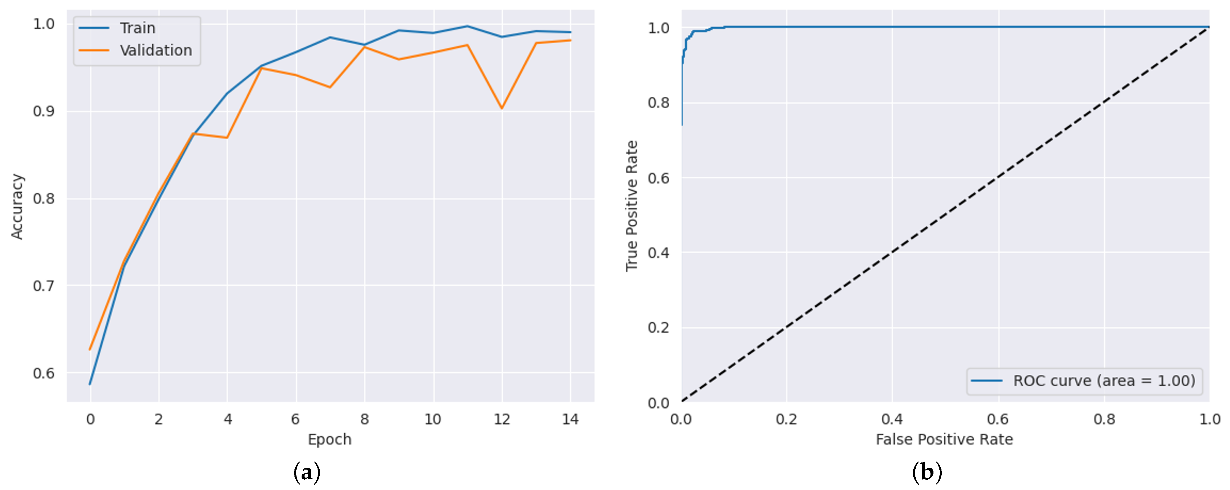
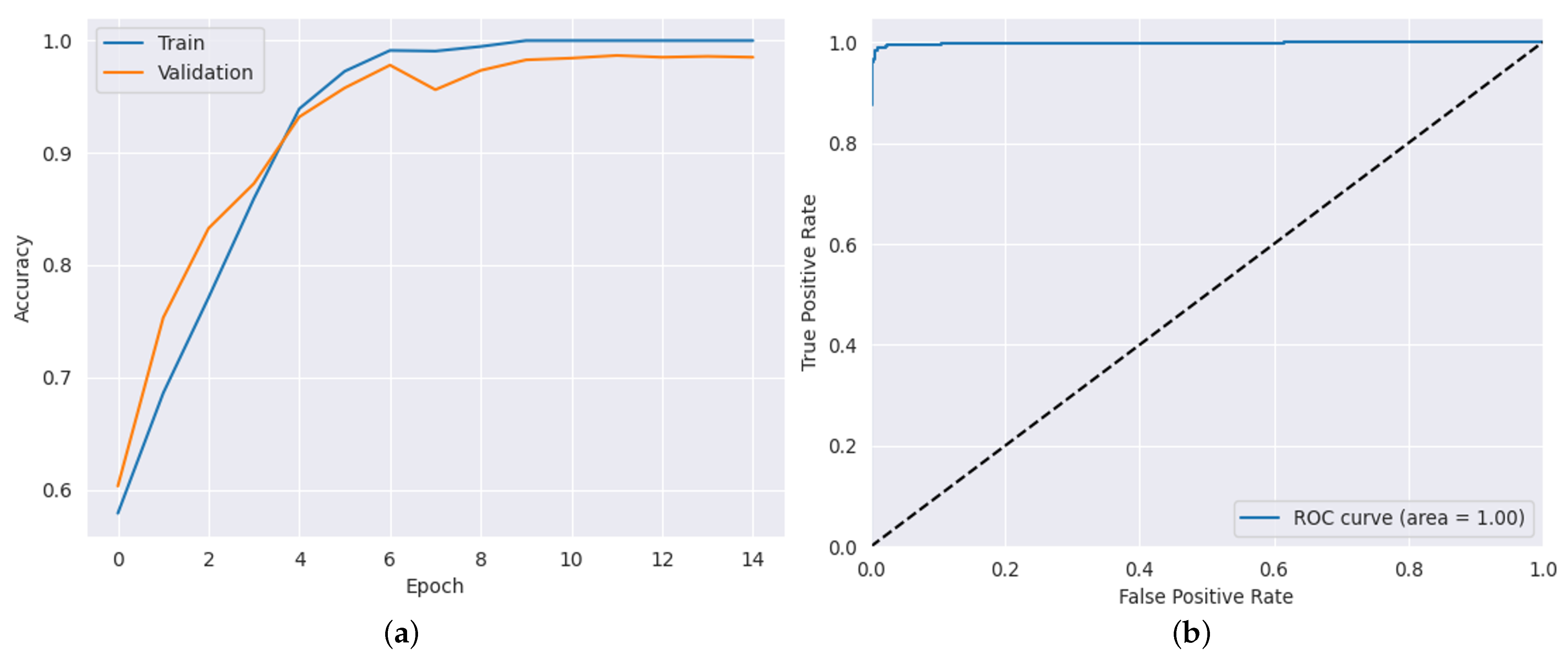
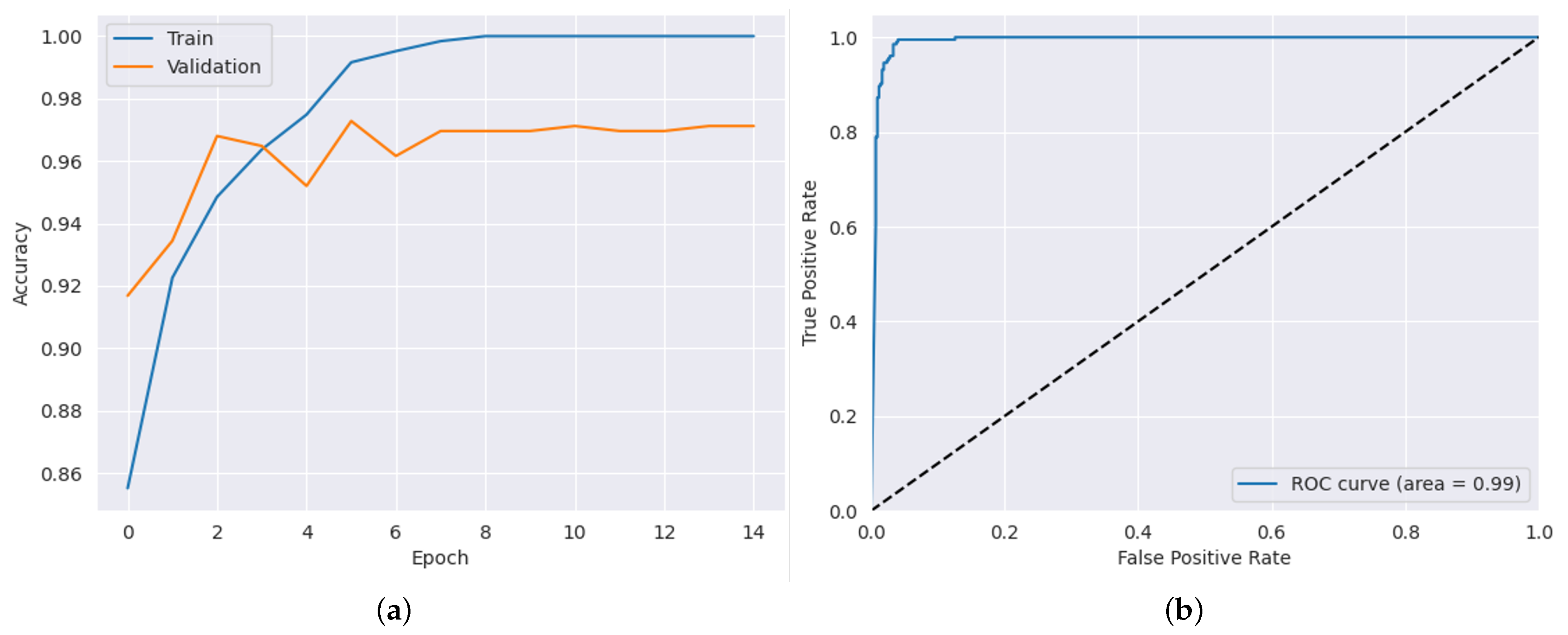
| Dataset | Metrics (%) | ||||
|---|---|---|---|---|---|
| Accuracy | Precision | Recall | AUC | False Negative Rate (FNR) | |
| ADNI Dataset | 98.50 | 97.53 | 98.60 | 99.83 | 1.72 |
| AD Dataset | 98.83 | 98.15 | 99.22 | 99.88 | 1.56 |
| Brain Tumor Dataset | 97.12 | 92.66 | 99.02 | 99.24 | 1.98 |
| Transfer Learning Model | Dataset | Metrics (%) | |||
|---|---|---|---|---|---|
| Accuracy | Precision | Recall | AUC | ||
| VGG16 | ADNI Dataset | 82 | 51.08 | 50.03 | 50.78 |
| AD Dataset | 82 | 50.61 | 62.66 | 50.61 | |
| Brain Tumor Dataset | 94 | 66.34 | 65.56 | 50.74 | |
| Inception V3 | ADNI Dataset | 50.50 | 49.50 | 50.26 | 48.07 |
| AD Dataset | 50.05 | 50.03 | 50.35 | 47.05 | |
| Brain Tumor Dataset | 90.03 | 68.49 | 68.06 | 49.54 | |
| ResNet50 | ADNI Dataset | 68 | 49.07 | 50.38 | 49.27 |
| AD Dataset | 69 | 51.03 | 51.19 | 51.40 | |
| Brain Tumor Dataset | 87 | 55.59 | 53.97 | 50.63 | |
Disclaimer/Publisher’s Note: The statements, opinions and data contained in all publications are solely those of the individual author(s) and contributor(s) and not of MDPI and/or the editor(s). MDPI and/or the editor(s) disclaim responsibility for any injury to people or property resulting from any ideas, methods, instructions or products referred to in the content. |
© 2023 by the authors. Licensee MDPI, Basel, Switzerland. This article is an open access article distributed under the terms and conditions of the Creative Commons Attribution (CC BY) license (https://creativecommons.org/licenses/by/4.0/).
Share and Cite
Ibrahim, R.; Ghnemat, R.; Abu Al-Haija, Q. Improving Alzheimer’s Disease and Brain Tumor Detection Using Deep Learning with Particle Swarm Optimization. AI 2023, 4, 551-573. https://doi.org/10.3390/ai4030030
Ibrahim R, Ghnemat R, Abu Al-Haija Q. Improving Alzheimer’s Disease and Brain Tumor Detection Using Deep Learning with Particle Swarm Optimization. AI. 2023; 4(3):551-573. https://doi.org/10.3390/ai4030030
Chicago/Turabian StyleIbrahim, Rahmeh, Rawan Ghnemat, and Qasem Abu Al-Haija. 2023. "Improving Alzheimer’s Disease and Brain Tumor Detection Using Deep Learning with Particle Swarm Optimization" AI 4, no. 3: 551-573. https://doi.org/10.3390/ai4030030