Cloud-Based Reinforcement Learning in Automotive Control Function Development

Abstract

Automotive control functions are becoming increasingly complex and their development is becoming more and more elaborate, leading to a strong need for automated solutions within the development process. Here, reinforcement learning offers a significant potential for function development to generate optimized control functions in an automated manner. Despite its successful deployment in a variety of control tasks, there is still a lack of standard tooling solutions for function development based on reinforcement learning in the automotive industry. To address this gap, we present a flexible framework that couples the conventional development process with an open-source reinforcement learning library. It features modular, physical models for relevant vehicle components, a co-simulation with a microscopic traffic simulation to generate realistic scenarios, and enables distributed and parallelized training. We demonstrate the effectiveness of our proposed method in a feasibility study to learn a control function for automated longitudinal control of an electric vehicle in an urban traffic scenario. The evolved control strategy produces a smooth trajectory with energy savings of up to 14%. The results highlight the great potential of reinforcement learning for automated control function development and prove the effectiveness of the proposed framework.

1. Introduction

In recent years, the automotive industry has undergone a significant transformation, with vehicles turning from mechanical systems into highly software-driven systems. Today, software has become the most important factor for automotive manufacturers [1], and approximately 80% of functions in the vehicle are realized through software [2]. A modern production vehicle usually has more than 100 electronic control unit (ECUs) with millions of code lines [3,4]. This already high level of complexity is projected to grow exponentially as software is becoming more and more interconnected, both within the vehicle and with external devices and because automated driving functions come with more extensive features and stricter regulations apply [1].

As the complexity of automotive software continues to rise, so does the importance of the underlying control algorithms inside the ECUs that operate the mechatronic subsystems of the vehicle by converting sensor information into control commands for the actuators. Thus, the control functions are ultimately responsible for the safe and eco-friendly vehicle operation and have a strong impact on the overall performance. In the conventional automotive software development process specified by the V model [5], the control function development occurs at an early stage of the process, usually involving model-in-the-loop (MiL) simulations. The resulting control function is then converted into machine code for the target hardware and deployed on an ECU, typically in a hardware-in-the-loop (HiL) environment first, where the subsequent calibration process for fine-tuning the control parameters begins [6]. Although certain steps of the development process, especially code generation and testing [7], are partly automated, the majority of the function development and calibration process is still highly dependent on human experts. The effort for these tasks, however, is continuously increasing, which is mainly caused by the rising complexity of function development [1] due to several factors. The urgent demand for sustainable transportation and the associated stricter regulations such as the expected Euro 7 emission standard are enhancing the performance requirements [8]. In addition, the growing number of ECUs sensors and actuators not only leads to additional functionality to be implemented, but also makes its development more difficult due to the manifold, intricate interactions with each other. At the same time, the number of vehicle variants and thus the need for specific, individual software is increasing [9]. Finally, the introduction of automated driving functions has led to a sharp increase in complexity due to the magnitude of sensor information and scenarios combined with high safety requirements [1]. As a result, function development is a time-consuming, costly process that poses challenges even for highly skilled professionals. In combination with steadily shortening product cycles and the general cost pressure, the process is prone to generation of suboptimal solutions that do not fully exploit the existing potential. Thus, the need for process automation is increasing in order to keep the effort at a feasible level and still obtain high-performing control functions.

Reinforcement learning (RL) constitutes a machine learning paradigm that aims to learn optimal control strategies [10]. In RL, an agent observes states from its environment and receives a feedback for its actions in the form of reward or punishment. Through interaction via trial-and-error, the agent derives its policy only from the experiences gathered during the training process. This ability to adapt to its environment and evolve end-to-end control strategies without human guidance makes RL particularly interesting for automation in the function development process. Due to the absence of tunable parameters of the derived control function, it combines both function development and calibration and thereby leads to a front-loading of the calibration process. By leveraging deep neural network (NNs), RL is particularly suited for automotive embedded systems with complex, non-linear environments and high-dimensional state and action spaces.

The aforementioned potentials of RL have led to a variety of applications in the context of automotive control.

Table 1. RL applications in the context of automotive control.

Simulation Software	Automated Driving	Actuator Control	Energy & Thermal Management
CARLA	[11,12,13,14,15]
CarSim	[16,17,18] *	[19] *	[20]
Gaming Engines	[21,22,23,24]
SUMO	[12,25,26,27,28]
MATLAB/Simulink	[18] *, [29]	[19,30,31,32] *, [33,34,35]	[36,37,38,39]
GT-Power		[30,31,32] *

* co-simulation.

shows common vehicular RL applications categorized by use case and, because all agents were trained in purely virtual environments, sorted by the utilized simulation software. The table is not intended to be a fully comprehensive review of all existing literature, but rather an overview and classification of common use cases.

RL-based automated driving is a very active field of research with numerous publications. Articles summarized in this column in Table 1 describe approaches where an RL agent directly affects the longitudinal or lateral motion of the vehicle, e.g., by controlling the desired longitudinal acceleration or the steering angle. Publications in this field encompass a wide range of applications, e.g., lane changing [15], ramp merging [27] or automated parking [18]. Additionally, these publications differ in terms of the scenarios they investigate, such as inner-city [29] or highway [23] driving, and their primary optimization targets, such as improving safety [14] or energy efficiency [28]. The choice of simulation tools depends on the specific purpose of the research. Automated driving relies heavily on an accurate perception, so a realistic 3D scenery and accurate sensor simulation is crucial for studies with realistic sensor vision. Therefore, the 3D simulations CARLA or CarSim are popular tools but gaming engines are also utilized frequently as they usually feature sophisticated graphics. Research with a stronger focus on strategic decision making, on the other hand, often employs the microscopic traffic simulation with Simulation of Urban Mobility (SUMO), as it realistically depicts the overall traffic dynamics. It is used either standalone, e.g., in traffic flow optimization [25], or in co-simulation, where it is responsible for simulating the surrounding traffic. MATLAB/Simulink, one of the most widely used tools in the automotive domain due to its high flexibility and customization capabilities, is used less frequently in this area of research.

The column actuator control in Table 1 refers to studies where an RL agent directly controls at least one active component of the vehicle. These use cases are usually characterized by the optimization of the control trajectory under external boundary conditions, e.g., a specific torque that needs to be produced. The literature provides the control of various actuators inside the powertrain, such as an active turbocharger or an exhaust gas recirculation (EGR) valve [30,31,33] of a combustion engine or the inverter of an electric motor [34]. Furthermore, applications outside the powertrain, such as an active steering system [19] or a semi-active suspension [35] control, can be found in the literature. Here, specialized simulations are utilized to model the specific system that contains the controlled component. This often involves developing custom models in MATLAB/Simulink or using specialized tools such as GT-Power for combustion engine modeling.

The third column covers automotive RL applications with a more strategic control task, operating the complete system rather than certain components. Among others, these include RL-based control strategies ([36,37,38]) for hybrid powertrain management as well as torque distribution [20] and thermal management [39] of electric vehicle (EVs). Similar to the actuator control, tools and simulation models here are more tailored to the specific use case.

Despite its undeniable potential and many promising proof-of-concept studies (see Table 1) that show the ability of RL agents to solve complex vehicular control problems, there are still some major challenges that prevent the wide-spread usage of RL in the automotive industry. One reason why RL still has a prototype status is that all studies use different tools that are suitable for the given use case but hard to transfer into a real application due to their incompatibility with the conventional development process. These tools are difficult to integrate into existing development pipelines, have real-time performance constraints, or are not compliant with industry standards and regulations. Furthermore, general safety concerns due to the RL agents’ black-box nature are present. The generalization capability and robustness of RL-based controllers can currently not be assured [40], so new testing methods must be established to guarantee safe operation across the complete spectrum of possible scenarios. Lastly, its trial-and-error approach results in a high demand for computationally expensive training episodes, often requiring thousands to solve even relatively simple problems, which exacerbates the difficult in its application to many different tasks.

Our contribution aims to lower the barriers of entry for RL-based control functions and attempts to bring them one step closer towards an application in production vehicles. We introduce a framework that is more tailored to the requirements of automated RL-based control function development and demonstrate a potential tooling solution. The central element is a connection between the open-source RL library RLlib and the commonly used and well-established dSPACE automotive development toolchain. By leveraging the associated automotive simulation models (ASM), which are commonly utilized in series development throughout the entire V-model, a seamless transfer to higher virtualization levels such as HiL can be realized. Further, the framework offers continuous variation of the simulated scenario and all model parameters as well as integrated testing capabilities to continuously monitor the agent’s performance and prove their robustness under different conditions. To be able to handle the high training demand, especially in computationally expensive tasks such as sensor simulation, we transfer the toolchain into the cloud for distributed parallel execution of the training and testing episodes. Another advantage of the toolchain is its flexibility both in terms of the use case and the RL algorithm. The vehicle for which the function is to be developed can be equipped with different sensors, powertrain topologies and software features. Thereby, all use cases listed in Table 1 could potentially be covered. Each simulated vehicle component has a clear separation between the plant and the control model, enabling an easy integration of an RL agent close to the real software structure. The general interface between the RL agent and the simulation also leaves flexibility in the choice of the model-free RL algorithm.

The paper is structured as follows: Section 2 gives a theoretical background of RL, before the framework including the simulation models, the cloud-setup, and the process flow are introduced. In Section 3, the framework is applied in a feasibility study to learn an inner-city driving function. Here, the scenario is introduced, before the RL problem is formulated and the results are discussed.

2. Methodology

The following chapter covers the integration of RL, the core methodology of our approach, into the automotive development toolchain.

2.1. Reinforcement Learning

RL is one of the three main paradigms of machine learning, along with supervised and unsupervised learning, which deals with an agent that freely interacts with an environment to gain experience that is later used to optimize the agent’s strategy. Central to this paradigm is the definition of the environment as a time-discrete Markov decision process (MDP) $(S,A,P,R)$, where S is the set of all states, A is the set of all actions, $P:S\times A\times S\to [0,1]$ is the transition probability function, and $R:S\times A\times S\to \mathbb{R}$ is the reward function. The agent’s policy is described by an action distribution ${\pi }_{\theta }:S\times A\to [0,1]$ with configurable parameters $\theta$. An experience is a single interaction $(s_t,a_t,s_{t+1},r_t)$, i.e., the state $s_t\in S$ the agent observes, the action $(a_t\in A)\sim {\pi }_{\theta }(·|s_t)$ it chooses, the successor state $(s_{t+1}\in S)\sim P(·|s_t,a_t)$ the environment transitions into, and the reward $r_t=R(s_t,a_t,s_{t+1})$ that is given for it. A sequence of interactions

$$\tau =\left((s_0,a_0,s_1,r_0),\dots ,(s_{T-1},a_{T-1},s_T,r_{T-1})\right)$$

(1)

from a start state $s_0\in S$ to a terminal state $s_T\in S$ is called an episode. RL strives to maximize the cumulative discounted episode reward

$$R\left(\tau \right)=\sum _{t=0}^{T-1}{\gamma }^t{r}_t$$

(2)

where $\gamma \in (0,1]$ is the discount rate. It does so by modifying the policy parameters $\theta$, e.g., via gradient ascent [10].

RL agents need an environment to interact with from which they learn to map inputs to outputs and thus represent the control function itself. Training on real hardware is time inefficient and costly, and in the case of autonomous driving, it is also highly safety critical. Therefore, RL agents are trained in simulation models.

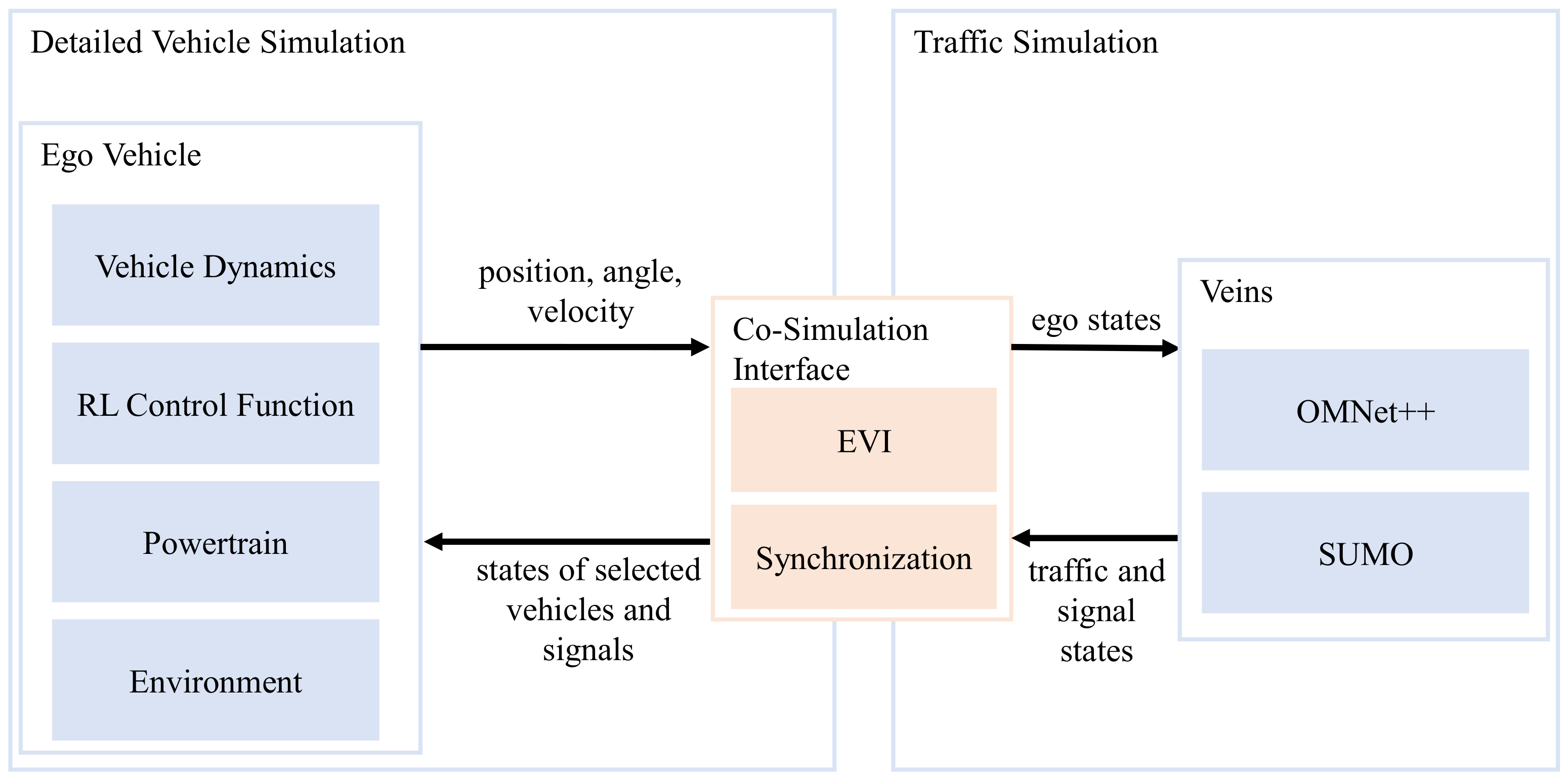
2.2. Simulation Environment

Developing control functions for automotive applications typically starts with defining the requirements and the use cases [41,42,43]. Based on these definitions, a suitable model has to be derived or selected to represent the behavior of the plant with a fidelity required by the function at hand. The level of fidelity also depends on the development stage and on whether an individual function is tested or multiple functions are integrated. Thus, a flexible model basis is required to provide a variable level of complexity, which allows control functions to be easily integrated to accelerate the development process. A test environment to meet those requirements is shown in Figure 1. It is based on the work by Eisenbarth et al. [44] and can be used on different platforms from MiL, software-in-the-loop (SiL) to HiL and vehicle-in-the-loop (ViL) as well as in local or cloud-based environments.

Main components of this test environment are the detailed vehicle simulation on the left, the traffic simulation on the right and the co-simulation interface coupling these two domains. The detailed vehicle simulation is based on the ASM tool suite and represent a high fidelity ego vehicle and environment real-time simulation model. The term ego vehicle is used for the vehicle for which the control function is to be developed. The RL control function comprises a use case independent RL block and individual, optional pre- and postprocessing functions as described in Section 2.3. The traffic simulation is based on Vehicles in Network Simulation (Veins) and utilizes SUMO to simulate a vast quantity of low fidelity vehicle models within a road network, whereas Objective Modular Network Testbed in C++ (OMNeT++) emulates the communication between static and dynamic objects. The co-simulation interface synchronizes both simulations and receives the state of the ego vehicle simulated in ASM and returns relevant traffic objects that are then perceived by the simulated sensors. Relevant traffic objects are chosen based on a minimal distance norm in a circular area around the ego vehicle, where an additional circle around the ego vehicle is defined to select the relevant nodes for vehicle-to-everything (V2X) communication. Both tasks are handled by the ego vehicle interface (EVI) [44].

Depending on the use case, relevant parts of the simulation environment can be used individually for function development or unit test and be integrated in a more complex environment when integrating different functionalities. For instance, an RL agent to control the engine can be trained using only the powertrain model of a single ego vehicle, whereas an RL agent controlling an automated vehicle requires a model of the vehicle dynamics and sensors, along with realistic traffic scenarios which may involve vehicle-to-infrastructure (V2I) communication. The simulation environment presented in this paper can be used for both use cases and its individual components are described in the following sections.

2.2.1. Physical Simulation

The ASM tool suite is the basis for the simulation models of vehicle dynamics, powertrain, sensors and environment as well as for soft ECUs, controlling the longitudinal or lateral motion of the vehicle. These components are based on open MATLAB/Simulink models, which are connected via bus interfaces and are separated in plant and control part, with interfaces to connect external control algorithms directly. Thus, individual subsystems can be replaced with models of a different level of fidelity or models implemented on a different basis, e.g., functional mock-up unit (FMU), robot operating system (ROS) or virtual electronic control unit (VECU). This structure can represent a truck with a diesel engine as well as a battery electric car and both types of vehicles can be used as ego vehicle in the test environment shown in Figure 1. The fidelity of the model can easily be adapted. For example, a mean-value engine model can be replaced by a model simulating the in-cylinder pressure. For higher level advanced driver assistance systems (ADAS) functions, line, traffic sign as well as sonar and radar sensors are available, together with an environment model and an electronic horizon, containing map information based on the v2 standard by the advanced driver assistance systems interface specification (ADASIS) consortium [45]. For realistic scenarios, the traffic participants and infrastructure around the ego vehicle are controlled by SUMO, as described in the following section.

2.2.2. Microscopic Traffic Simulation

The traffic flow and communication simulation is based on the open-source software environment Veins 5.0, connecting SUMO 1.13.0 for traffic and OMNeT++ 5.6.2 for network communication simulation. This enables the simulation of realistic traffic scenarios, including communication between vehicles as well as between vehicles and infrastructure. For instance, scenarios can represent rush hour in a city and be used for powertrain function development with a realistic load cycle as well as for automated driving functions controlling vehicles in dense traffic without the need for individually modeling the behavior of the surrounding vehicles. SUMO simulates the movement of individual traffic participants through a given road network. The traffic demand can be multimodal, and each participant has its own route and obeys traffic rules and lights. Every traffic participant is also represented by a node in OMNeT++, where the communication is simulated including interference effects and shadowing by other moving objects or buildings. Figure 2 illustrates the co-simulation of ASM and SUMO. On the left, the ASM simulation is visualized by MotionDesk where the blue ego vehicle can be seen. This vehicle is shown on the right side as a yellow vehicle in the SUMO graphical user interface (GUI). The synchronized states of the traffic light are also highlighted in both simulation tools.

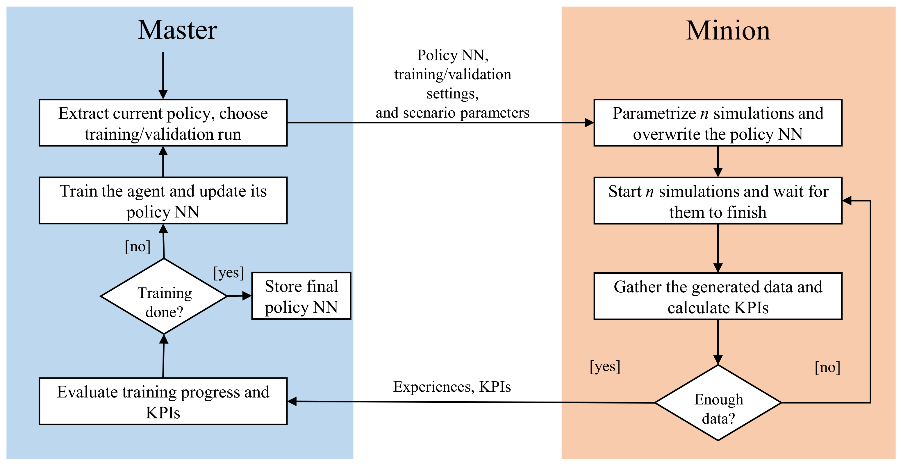
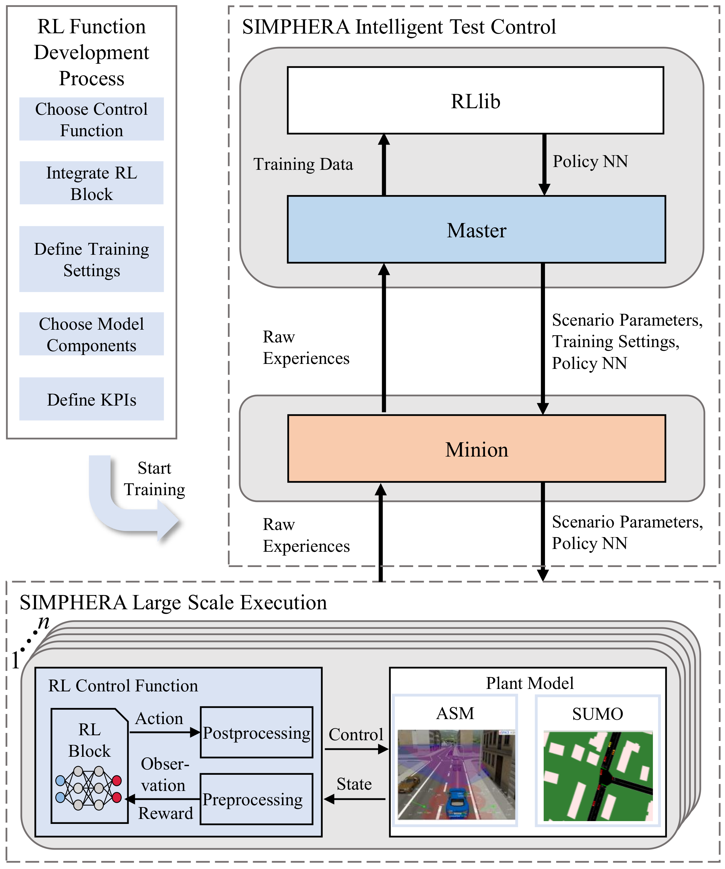
2.3. Distributed Learning Framework

To overcome the challenges of on-policy data generation and model execution speed, as outlined in Section 2.1, a cloud setup as well as a proprietary software interface has been developed. Basis for the cloud setup is SIMPHERA [46], which offers a web-based interface for parametrization, parallel simulation and analysis of individual scenarios.

The proprietary software interface is based on a master–minion architecture. Figure 3 illustrates the training process, which is managed by the master in a cyclic manner: At the beginning of each cycle, the master extracts the policy NN and sends it to the minion along with the training and scenario parameters to concertize the logical scenario used for simulation. This prompts the minion to start a configurable number n of parallel simulations, each tasked with completing an episode, and to wait for them to finish. Should the number of generated experiences not be sufficient after they have terminated (e.g., if the model entered a catastrophic state and therefore a simulation could not continue), the minion starts additional simulations. Once the necessary amount of data has been collected, it is sent back to the master via TCP/IP using a custom protocol. Subsequently, the master interfaces the open-source library RLlib [47] and trains the agent with the data the minion generates. After updating the agent, the cycle starts again. Besides these training cycles, so called validation cycles are performed continuously after a pre-defined number of training cycles. The difference between the two types is that, during validations, only one simulation is performed, and in this simulation, the agent’s actions are not sampled stochastically according to ${\pi }_{\theta }$, but rather by just taking the policy’s mean. Thus, a more comparable snapshot of the agent’s performance and a reproducible behavior of the control function are attained. Additionally, key performance indicator (KPIs) can be defined to assess the performance of the control function during a validation run. These KPIs can be used to stop the training process once an agent has been trained sufficiently according to the requirements defined earlier.

The training process described above is orchestrated by SIMPHERA, using its intelligent test control interface to execute simulations, calculate KPIs, and collect results. This cloud setup is shown in Figure 4, together with the workflow for developing an RL-based control function on the left. Initially, the function to be controlled is defined and an RL block and optional pre- and postprocessing functions are integrated into the corresponding control function model (c.f. Figure 1). Next, the training is configured by selecting the relevant component of the plant model and the scenario, defining KPIs and stating the training settings including the definition of the state and action space as well as the reward function. After these manual steps are accomplished, the presented framework starts to generate the control function automatically and no further human intervention is required. Initiating a training configured this way, SIMPHERA starts and configures containers in a cloud environment for master and minion, before the training process shown in Figure 4 is conducted, wherein individual containers are highlighted with a gray background. During training, SIMPHERA combines the individual components of the plant model and control function into one joint application and starts a large-scale execution of the application with n simulation containers composed of the setup in Figure 1. This step also includes the concretization of the logical scenario, where each simulation instance receives a different concrete scenario, allowing for a broad bandwidth of situations. Thus, the generalizability of the agent is also promoted, so that it achieves a better performance in unknown situations. The central component of the control function is the RL block, which is responsible for executing the policy NN, storing experiences and sampling the action according to the applied RL algorithm. The weights and biases of the policy NN are send to the minion for each cycle. Because the RL block uses TensorFlow Light Micro [48] and is written in C++, the RL-based control function can be easily compiled for real time prototyping hardware. The RL block can be accompanied by customized modules for pre-processing observations (e.g., min–max normalization) or post-processing the actions (e.g., denormalization or safety filtering), but can also be executed standalone when learning an end-to-end policy. After an episode is finished, the calculated KPIs and experiences are sent to the minion. Because this simulation is based on a containerized architecture, it can be scaled freely according to the available cloud resources. Once the master determines a sufficient training progress based on the KPIs defined, the large-scale simulation and intelligent test control is shut down and the final policy NN as well as the training results are stored.

3. Feasibility Study

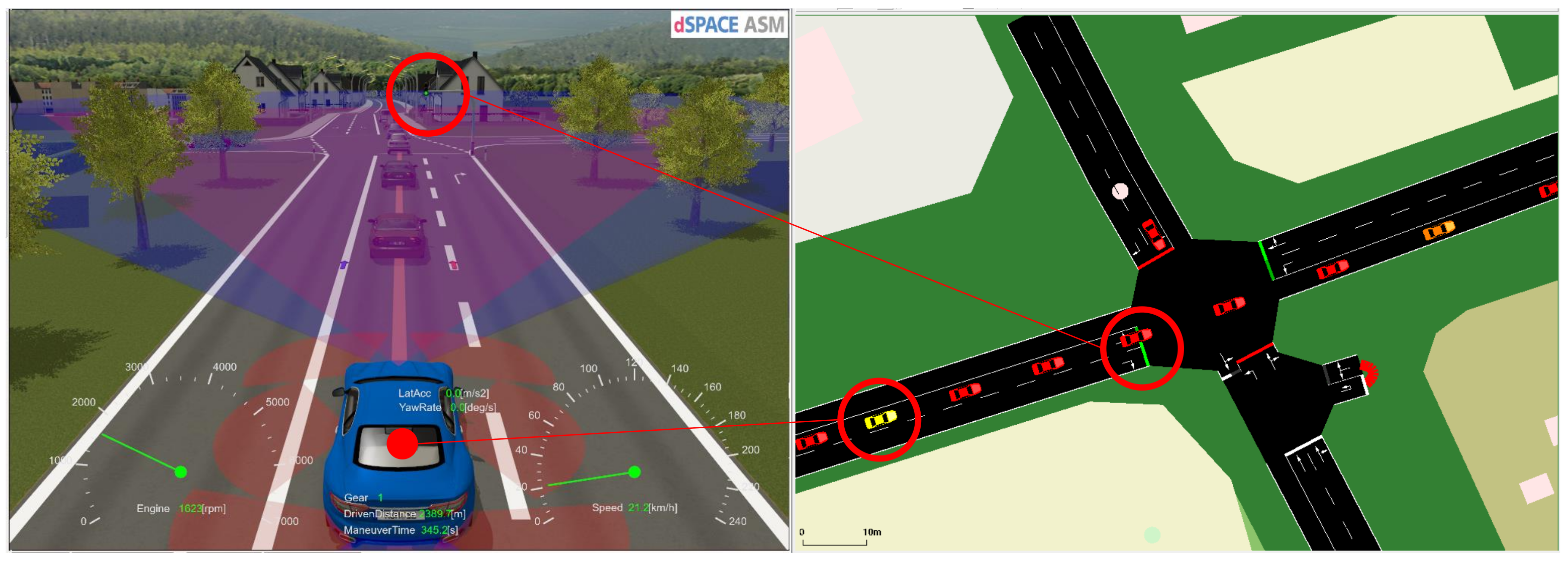
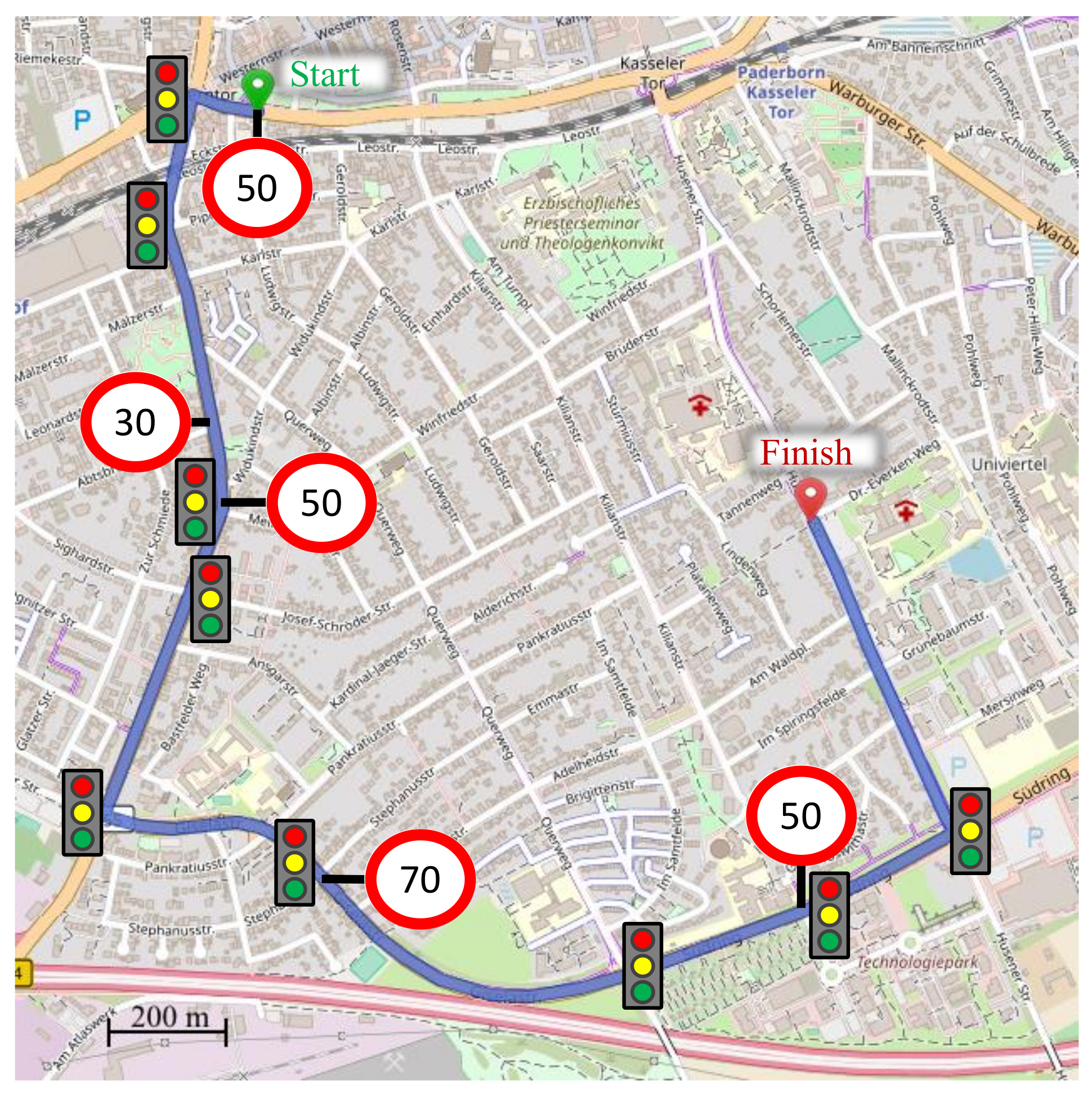
To showcase a potential application of the framework introduced in the previous chapter, an exemplary feasibility study was conducted. Here, a longitudinal controller for an automated vehicle represents the control function to be developed using RL and the presented simulation toolchain. The controller has the goal to generate a smooth and energy-efficient trajectory while considering different safety aspects.

3.1. Scenario

For the training and validation of the agent, a route was selected on which the ego vehicle, simulated in ASM, interacts with other traffic participants and traffic lights controlled by SUMO.

3.1.1. Route

The simulation environment is based on a real road network in Paderborn, a medium-sized city in Germany, described in [49], where the traffic volume is calibrated to match actual traffic measurements. All traffic lights along the route are switched with a 90 s cycle period and a yellow-light phase with a duration of 3 $\mathrm{s}$ is present at the transition from red to green. Within this scenario, a route representative for a typical inner-city drive with a length of $3.7$ $\mathrm{k}$$\mathrm{m}$ is selected. Along the route, different speed-limited zones (30, 50, and 70/$\mathrm{h}$) and different number of lanes (1–2) occur. Further, it contains 9 signalized and 18 unsignalized intersections. There is right of way along the entire route and all left-turning traffic lights are exclusive. The route with all features is depicted in Figure Figure 5.

3.1.2. Ego Vehicle

The ASM suite is configured to model the ego vehicle as an EV with a single permanent magnet synchronous motor. The motor is connected to the rear wheels via a differential with an integrated single-stage gear set. All vehicle and powertrain parameters are calibrated to match a BMW i3 vehicle and are listed in

Table A1. Overview of ego vehicle, sensor and environment data.

Subject	Data	Value
Vehicle Dynamics	cW-value	0.27
	Frontal area	2.38 ${\mathrm{m}}^2$
	Unladen weight	1345 $\mathrm{kg}$
	Acceleration 0 to 60 $\mathrm{km}$ ${\mathrm{h}}^{-1}$	3.5 $\mathrm{s}$
	Top speed	150 $\mathrm{km}$ ${\mathrm{h}}^{-1}$
Powertrain	Motor power (rated/peak)	75/125 $\mathrm{kW}$
	Motor torque	250 $\mathrm{Nm}$
	Transmission ratio	9.75
	Battery capacity	42 $\mathrm{kW}$ $\mathrm{h}$
	Battery technology	Lithium-ion
Camera Sensor	Range	50 $\mathrm{m}$
	Sensor position/direction	front/front
Radar Sensor	Range	150 $\mathrm{m}$
	Sensor position/direction	front/front
V2I	SPaT message
E-Horizon	ADASIS v2 Standard [45]

. To be as close as possible to the real application, the ego vehicle is equipped with various, non-ideal environment sensors. The radar sensor enables the detection of vehicles located up to 150 $\mathrm{m}$ in front of the ego-vehicle and provides a list of up to 15 objects. Each object is characterized by type, which contains the information if the object is a vehicle and its velocity as well as its position relative to the ego vehicle. The camera sensor provides the position of the ego lane boundaries at a distance of 10 $\mathrm{m}$–50 $\mathrm{m}$ in front of the ego vehicle. For this purpose, the positions of 5 equidistant points on each side of the lane are obtained. Both sensors are located at the front of the vehicle and consider effects such as masking and noise. In addition, the ego vehicle incorporates an electronic horizon and receives signal phase and timing (SPaT) messages via V2I. The lateral control of the ego vehicle is performed by a conventional lane keeping controller.

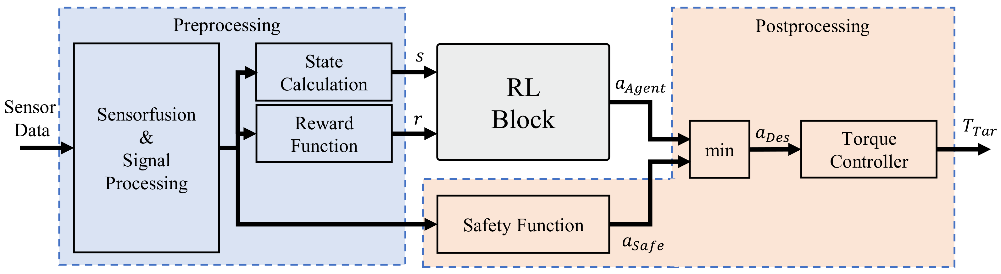
3.1.3. RL Control Function

The task of the control function, which represents the system to be developed, is to provide safe, efficient longitudinal guidance of the vehicle by determining a target torque as a function of the given sensor information. The functional architecture is shown in Figure 6 and can be logically divided into the three parts preprocessing, RL block and postprocessing. The sensor data is preprocessed by a fusion algorithm that matches the camera’s lane information with the object list from the radar sensor to find the relevant target vehicle. Further, information about road curvature, speed limits, road slope and traffic light states along the upcoming segments are extracted from the electronic horizon and the V2I messages, respectively. These processed data are then used to calculate the state signals s and the reward r for the current time step (see Section 3.2). These two quantities are input into the RL block where they are sampled and then used to determine the agent’s action, the desired acceleration of the ego vehicle $a_{Agent}$.

In parallel, the safety function ensures safe driving conditions by calculating a safe acceleration request $a_{Safe}$. Here, the following safety criteria are considered:

• Collision: safety time gap (1 $\mathrm{s}$) and distance (1 $\mathrm{m}$) to the preceding vehicle are assured.
• Speed limit: compliance with legal speed limits is guaranteed.
• Curvature: the curve speed is limited to ensure that a lateral acceleration of 3 $\mathrm{m}$ ${\mathrm{s}}^{-2}$ is not exceeded.
• Traffic light: red-light violations are prevented.

For each item, a kinematic model of the ego vehicle is used to calculate the maximum acceleration at which the respective criterion is just fulfilled. $a_{Safe}$ then equals the minimum of these four calculated acceleration values. The acceleration request $a_{Des}$, which is formed from the minimum of $a_{Agent}$ and $a_{Safe}$ to prevent the agent from entering safety-critical driving states, is then converted into a target torque $T_{Tar}$ by a downstream PI-controller. This target torque is fed back into the simulation environment and affects the motion of the vehicle to close the control loop.

3.2. Problem Formulation

The definition of the agent’s interface to the environment and the choice of a suitable RL algorithm is a crucial step that needs to be performed manually at an early stage of the RL-based function development process. The state space (see

Table 2. Overview of the RL agent’s state and action space.

Type	Quantity	Range
State	Ego velocity	0 $\mathrm{km}$ ${\mathrm{h}}^{-1}$ to 75 $\mathrm{km}$ ${\mathrm{h}}^{-1}$
	Ego longitudinal acceleration	−4 $\mathrm{m}$ ${\mathrm{s}}^{-2}$ to 3 $\mathrm{m}$ ${\mathrm{s}}^{-2}$
	Ego lateral acceleration	−3$\mathrm{m}$ ${\mathrm{s}}^{-2}$ to 3 $\mathrm{m}$ ${\mathrm{s}}^{-2}$
	Fellow distance	0 $\mathrm{m}$ to 150 $\mathrm{m}$
	Fellow relative velocity	−70 $\mathrm{km}$ ${\mathrm{h}}^{-1}$ to 70 $\mathrm{km}$ ${\mathrm{h}}^{-1}$
	Traffic-light status	0 or 1
	Traffic-light switching time	0 $\mathrm{s}$ to 70 $\mathrm{s}$
	Traffic-light distance	0 $\mathrm{m}$ to 300$\mathrm{m}$
	Current legal speed limit	0 $\mathrm{km}$ ${\mathrm{h}}^{-1}$ to 70 $\mathrm{km}$ ${\mathrm{h}}^{-1}$
	Distance to upcoming legal speed limit	0 $\mathrm{m}$ to 150 $\mathrm{m}$
	Upcoming legal speed limit	0 $\mathrm{km}$ ${\mathrm{h}}^{-1}$ to 70 $\mathrm{km}$ ${\mathrm{h}}^{-1}$
	Distance to velocity curvature limit	0 $\mathrm{m}$ to 150 $\mathrm{m}$
	Curvature speed limit	0 $\mathrm{km}$ ${\mathrm{h}}^{-1}$ to 70 $\mathrm{km}$ ${\mathrm{h}}^{-1}$
	Safe acceleration ($a_{Safe}$)	−4 $\mathrm{m}$ ${\mathrm{s}}^{-2}$–3$\mathrm{m}$ ${\mathrm{s}}^{-2}$
	Velocity band lower limit	0 $\mathrm{km}$ ${\mathrm{h}}^{-1}$ to 70 $\mathrm{km}$ ${\mathrm{h}}^{-1}$
	Velocity band upper limit	0 $\mathrm{km}$ ${\mathrm{h}}^{-1}$ to 70 $\mathrm{km}$ ${\mathrm{h}}^{-1}$
	Road slope	−30% to 30%
Action	Desired acceleration ($a_{Des}$)	−2 $\mathrm{m}$ ${\mathrm{s}}^{-2}$ to 3.5 $\mathrm{m}$ ${\mathrm{s}}^{-2}$

) contains the dynamic state of the ego vehicle and information from the environment sensors that are required to generate a safe longitudinal trajectory. The traffic light status indicates whether crossing the traffic light in the current lane is permitted. In combination with the next switching time and the distance, it enables generating an anticipatory driving trajectory. A velocity band with an upper ($v_{\mathrm{B},\mathrm{u}}$) and lower ($v_{\mathrm{B},\mathrm{l}}$) limit is defined to guide the agent towards arriving at traffic lights during a green phase. They are determined once when a new traffic light is detected by calculating the required velocities for earliest and latest arrival based on the distance and switching time information under consideration of the speed limits ahead. Both upper and lower speed limits can only be within a range of 70% to 100% of the permissible maximum speed, so as not deviate too much from human driving behavior. Furthermore, the current safe acceleration from the safety-function is used to provide information about the criticality of the current driving state. The state signals are passed to the RL block, where they are used to provide an acceleration demand $a_{Agent}$ as action within a sample time of $0.2$ $\mathrm{s}$. All state variables are min–max normalized according to the ranges stated in Table 2.

The reward function consists of multiple terms to serve different objectives. The first term of the reward function penalizes unsafe acceleration requests if the desired acceleration $a_{\mathrm{Agent}}$ exceeds the safety-function acceleration limit $a_{\mathrm{Safe}}$. The deviation of the ego vehicle velocity $v_{Ego}$ to the upper and lower velocity band limits $v_{\mathrm{B},\mathrm{u}}$ and $v_{\mathrm{B},\mathrm{l}}$ is taken into account to guide the agent towards an efficient velocity trajectory and accelerate the training. Sanctioning the ego vehicle’s acceleration $a_{Ego}$ ensures a smooth movement. The successful crossing of a traffic light intersection $b_{TL}$ is rewarded as an encouragement to maximize the traveled distance. The individual terms of the reward function are weighted using the factors $f_{\mathrm{SF}}$, $f_{\mathrm{v}}$, $f_{\mathrm{a}}$, and $f_{\mathrm{TL}}$. The complete reward function is therefore defined as:

$$r=-f_{\mathrm{SF}}\tanh \left(\max (0,a_{\mathrm{Agent}}-a_{\mathrm{Safe}})\right)-f_{\mathrm{v}}{\max (0,v_{Ego}-v_{\mathrm{B},\mathrm{u}},v_{\mathrm{B},\mathrm{l}}-v_{Ego})}^2-f_{\mathrm{a}}{a}_{Ego}^2+f_{\mathrm{TL}}{b}_{\mathrm{TL}}$$

(3)

The model-free, on-policy RL algorithm proximal policy optimization (PPO) is selected for the feasibility study. Although the on-policy nature of PPO tends to make the algorithm more data inefficient compared to state-of-the-art off-policy algorithms, PPO stands out in different areas: first, it has a relatively low number of hyperparameters; hence, the training process is easy to set up. Second, it is a stable algorithm due to the fact that it optimizes a surrogate objective function which prevents huge update steps. [51] A fully connected tanh-activated feed-forward NN with 3 layers, each consisting of 16 nodes, is utilized as the policy networks inside the RL block.

3.3. Results

This section discusses the results of the feasibility study obtained with the cloud-based framework presented in Section 2. Both the training of the agent and the validation are executed via the route defined in Section Section 3.1.

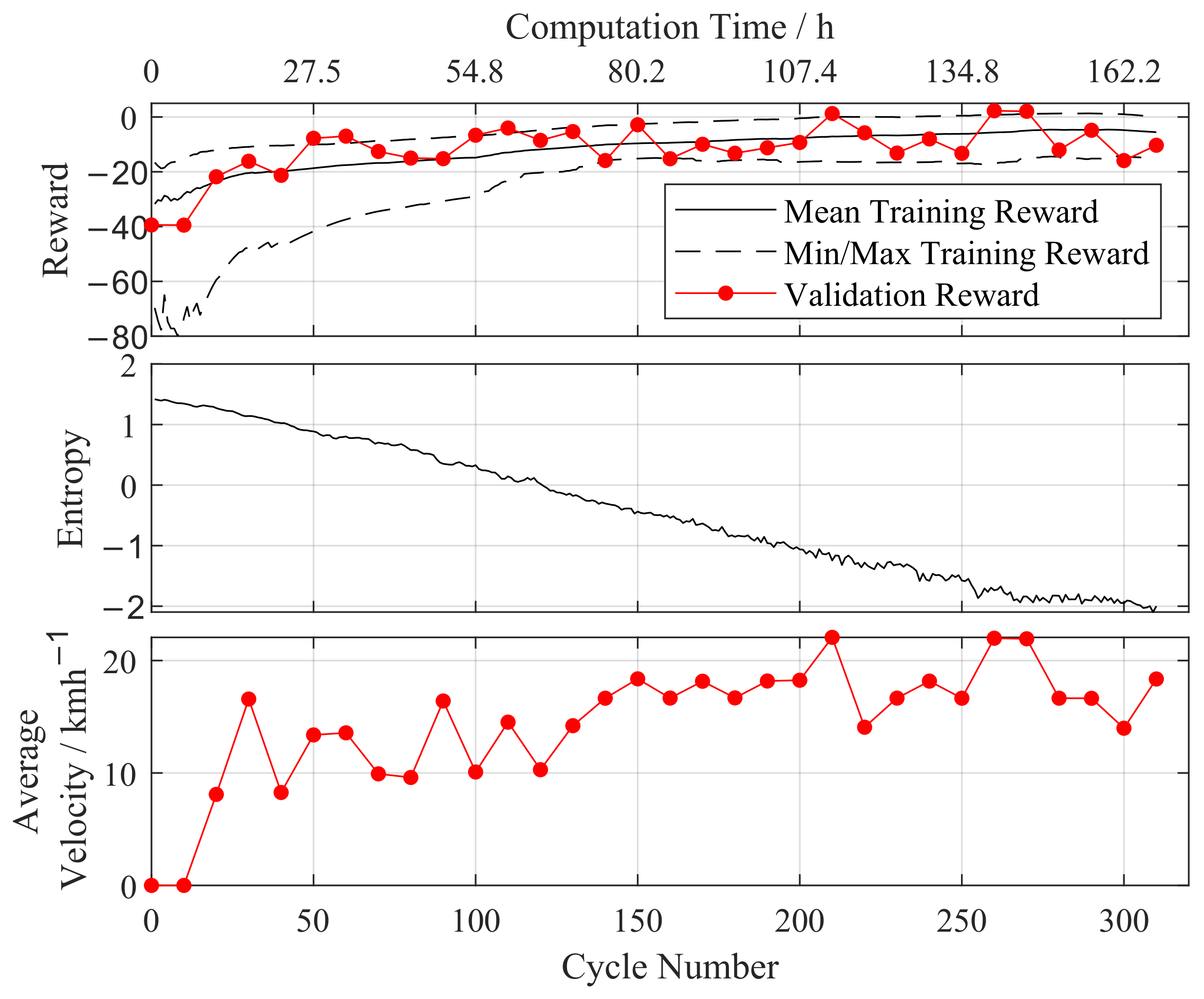
3.3.1. Training Results

The ASM-SUMO co-simulation is distributed over 10 simulation nodes that calculate the episodes in parallel. Each episode has a maximum length of 600 s simulation time, which is equivalent to 3000 samples. In case the vehicle has reached its terminal position earlier or one of the minions has crashed during the training episode, new episodes are started until the number of samples requested by the master is reached.

Figure 7 shows the training and validation progress, both in terms of training cycles and training duration in real time. All quantities obtained from the training episodes are marked in black, whereas the red points represent results of the validation runs that are executed after each tenth training cycle and therefore highlighted with a dot. The upper plot contains the minimum, maximum and mean cumulative reward of the 10 training episodes of each cycle as well as the total reward within the validation episodes. The average reward increases relatively strongly in the first cycles and then plateaus as the training duration progresses. It reaches its maximum after around 280 cycles and then begins to decline slightly until the training is stopped after 310 cycles. This trend is replicated in the validation episodes with minor deviations resulting from the deactivation of the action sampling. Furthermore, the range between the minimum and maximum reward is decreased during the training as the variance in the action steadily diminishes while the agent becomes more experienced. This is indicated by the decreasing entropy in the middle plot of Figure Figure 7. The lower plot shows the average velocity as an examplary KPI that is monitored during the training. It takes around 200 cycles for the agent to learn to complete the entire route. In general, these KPIs can be used to evaluate the training progress with regard to predefined control objectives.

Computing the 310 cycles took a total of 160 $\mathrm{h}$, approximately one week. Despite some minor random deviations caused by slightly varying simulation times and overhead, the training time is proportional to the cycles. The total execution time over all simulation instances was 1212 $\mathrm{h}$. Training, parametrization, model download and result upload as well as validation runs took about 25% of the total execution time, whereas 75% of the time has been used for parallel simulation. By distributing the simulation to 10 nodes, the total training is thus accelerated by a factor of 7.5, demonstrating the effectiveness of the distributed training approach. It must be taken into account that the cloud system has been optimized for minimal operating cost and not for computational power. Increasing the computational power and distributing additional nodes for parallel simulation can further decrease the time required for training.

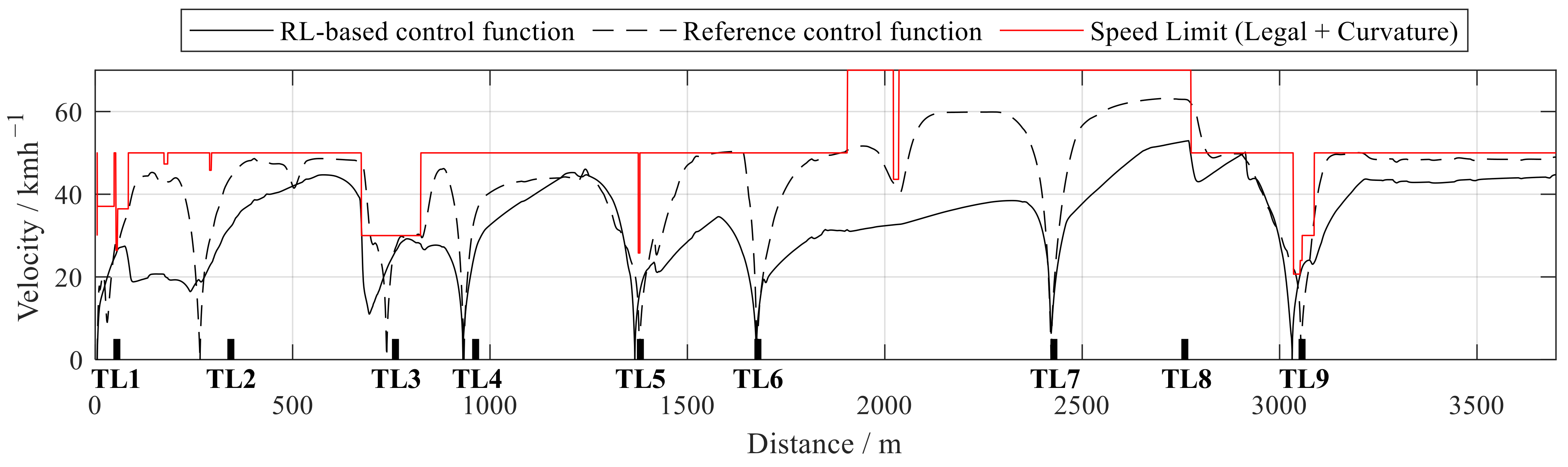
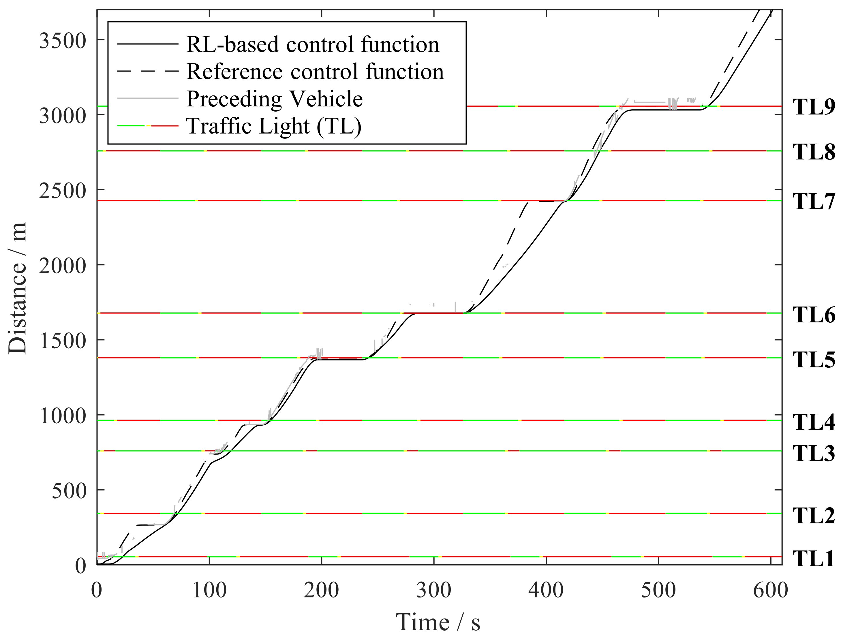
3.3.2. Validation Results

A validation run of the best performing agent from the training phase is used for an analysis of the evolved strategy. A rule-based control function based on the intelligent driver model (IDM) [52] (see Appendix B) with the parameters shown in

Table A2. IDM parameters.

Parameter	Description	Value
a	Maximum Acceleration	3.5 $\mathrm{m}{\mathrm{s}}^{-2}$
b	Comfortable Deceleration	2.5 $\mathrm{m}{\mathrm{s}}^{-2}$
T	Time headway	1 $\mathrm{s}$
$d_0$	Minimum distance	2 $\mathrm{m}$
$\delta$	Acceleration exponent	3.25

, modified to consider traffic lights and velocity restrictions, is chosen as a reference. For a fair comparison, the simulations with the RL-based and the IDM-based controllers are conducted using the same traffic scenario and initial conditions. All metrics evaluated in this chapter refer to a single drive along the $3.7$ $\mathrm{k}$$\mathrm{m}$ route shown in Figure 5.

Figure 8 shows the speed profile of the RL-based and the reference control function. The red line represents the minimum of the legal speed limit and the curvature speed limit. The locations of the traffic lights are marked at the x-axes. It can be seen that the agent operates the vehicle in accordance with the given velocity boundaries. However, the agent did not complete the route entirely without safety function interventions. At traffic lights 4 and 7, minor interventions are still required to regulate the exact stopping position behind the preceding vehicle. Exceeding the legal speed limit is prevented before traffic light 3 and twice after traffic light 8. No safety interventions are necessary to adjust the cornering speed or to prevent red light violations. A comparison of the velocity trajectories reveals that the agent tends to accelerate and decelerate less and reaches a lower maximum speed. While the reference control function fully exploits the velocity boundaries and thus the vehicle is forced to brake more frequently, the RL-based control function usually maintains a larger distance to the speed limit. This allows the agent to pass the first three traffic lights without a stop and a subsequent acceleration phase and generally reduces the necessity to brake for speed limit reductions or slower preceding vehicles.

The s–t diagram in Figure Figure 9 visualizes the position of the ego vehicle over time for the two control functions in relation to the traffic lights and the preceding vehicle as perceived by the radar sensor in the RL controlled scenario. When no gray line is present, no preceding vehicle is detected within the sensors range. This demonstrates the agent’s ability to handle the noisy sensor data. The agent tends to leave a relatively large gap between the preceding vehicle, but then catches up at the next red traffic light. With this strategy, the agent does not only avoid stops at traffic lights 1–3, but also reduces the waiting time on other traffic lights (4, 6, 9). Despite fewer standstill phases, the RL-based control strategy exhibits a 37% lower absolute acceleration on average and a more uniform speed profile compared to the IDM-based controller. This means that less lossy energy conversion from mechanical to electrochemical energy and vice versa is required. In combination with the lowered driving resistances resulting from the reduced maximum vehicle speed, the wheel energy demand is strongly reduced. In total, the energy consumption is lowered by 14%, from 16.2 to $13.9$ $\mathrm{k}$$\mathrm{W}$$\mathrm{h}$ per 100 $\mathrm{k}$$\mathrm{m}$, with almost identical travel times (IDM: 590 $\mathrm{s}$, RL: 602 $\mathrm{s}$).

4. Discussion and Outlook

In this article, an attempt integrating reinforcement learning into the automotive control function development process is presented. The proposed framework represents the first coupling of RL and a production-level, automotive development toolchain. The methodology shows a possible setup and architecture for an RL integrated solution and provides a first set of process steps for an RL-based development process. The combination of the dSPACE Automotive Simulation Models tool suite with its diverse set of models and the microscopic traffic simulator SUMO offers great flexibility in the control function domain and realistic scenarios for various applications. By utilizing distributed cloud simulations to meet the high demand for computationally intensive training episodes, RL-based control functions can be generated within a reasonable time frame, as demonstrated in the feasibility study. The compatibility of the simulation tools to the automotive development process would now enable a seamless transfer of the evolved control function to the next development stage, for example in a HiL environment. A valuable extension to be considered in future work is the introduction of an automated hyperparameter tuning procedure. For the presented feasibility study, the choice of hyperparameters for the RL algorithm and the reward function was still performed manually. For future applications, another automation layer shall be added to the framework to distribute not only training episodes, but complete training with different hyperparameters. Additionally, enhancing the tool’s user-friendliness through the development of a general user interface and automating the process of equipping models with the RL block would further streamline the workflow.

The feasibility study shows that the setup is working and that it is capable of automatically generating a control function for a complex control problem. However, it still offers improvement potential, as the agent so far is only trained and validated in a single scenario. The future focus will be on automatically generating driving scenarios to evolve a more generalized control function. Further, the current RL-based controller still relies to a significant extend on manually created functions such as the sensor fusion and the safety function. Therefore, the future goal is to develop an end-to-end policy that directly learns from the raw sensor information and only requires minor state preparation. Lastly, future work will make use of the toolchain’s flexibility regarding the computing hardware and virtualization level and will focus on evaluating the capabilities of the RL-based controller in real-world scenario by deploying it in a real vehicle using vehicle-in-the-loop simulation.

References

1. Ebert, C.; Favaro, J. Automotive software. IEEE Softw. 2017, 34, 33–39. [Google Scholar] [CrossRef]
2. Vogel, M.; Knapik, P.; Cohrs, M.; Szyperrek, B.; Pueschel, W.; Etzel, H.; Fiebig, D.; Rausch, A.; Kuhrmann, M. Metrics in automotive software development: A systematic literature review. J. Softw. Evol. Process 2021, 33, e2296. [Google Scholar] [CrossRef]
3. Antinyan, V. Revealing the complexity of automotive software. In Proceedings of the 28th ACM Joint Meeting on European Software Engineering Conference and Symposium on the Foundations of Software Engineering, Virtual, 8–13 November 2020; pp. 1525–1528. [Google Scholar]
4. Greengard, S. Automotive systems get smarter. Commun. ACM 2015, 58, 18–20. [Google Scholar] [CrossRef]
5. Möhringer, S. Entwicklungsmethodik für Mechatronische Systeme; Heinz-Nixdorf Institut: Paderborn, Germany, 2004. [Google Scholar]
6. Isermann, R. Automotive Control: Modeling and Control of Vehicles; Springer: Berlin/Heidelberg, Germany, 2022. [Google Scholar]
7. Juhnke, K.; Tichy, M.; Houdek, F. Challenges concerning test case specifications in automotive software testing: Assessment of frequency and criticality. Softw. Qual. J. 2021, 29, 39–100. [Google Scholar] [CrossRef]
8. Claßen, J.; Pischinger, S.; Krysmon, S.; Sterlepper, S.; Dorscheidt, F.; Doucet, M.; Reuber, C.; Görgen, M.; Scharf, J.; Nijs, M.; et al. Statistically supported real driving emission calibration: Using cycle generation to provide vehicle-specific and statistically representative test scenarios for Euro 7. Int. J. Engine Res. 2020, 21, 1783–1799. [Google Scholar] [CrossRef]
9. Mattos, D.I.; Bosch, J.; Olsson, H.H.; Korshani, A.M.; Lantz, J. Automotive A/B testing: Challenges and lessons learned from practice. In Proceedings of the 2020 46th Euromicro Conference on Software Engineering and Advanced Applications (SEAA), Portoroz, Slovenia, 26–28 August 2020; pp. 101–109. [Google Scholar]
10. Sutton, R.S.; Barto, A.G. Reinforcement Learning: An Introduction, 2nd ed.; The MIT Press: Cambridge, MA, USA, 2018. [Google Scholar]
11. Cao, Z.; Xu, S.; Peng, H.; Yang, D.; Zidek, R. Confidence-aware reinforcement learning for self-driving cars. IEEE Trans. Intell. Transp. Syst. 2021, 23, 7419–7430. [Google Scholar] [CrossRef]
12. Gutiérrez-Moreno, R.; Barea, R.; López-Guillén, E.; Araluce, J.; Bergasa, L.M. Reinforcement learning-based autonomous driving at intersections in CARLA simulator. Sensors 2022, 22, 8373. [Google Scholar] [CrossRef]
13. Li, D.; Okhrin, O. Modified DDPG car-following model with a real-world human driving experience with CARLA simulator. Transp. Res. Part C Emerg. Technol. 2023, 147, 103987. [Google Scholar] [CrossRef]
14. Cao, Z.; Bıyık, E.; Wang, W.Z.; Raventos, A.; Gaidon, A.; Rosman, G.; Sadigh, D. Reinforcement learning based control of imitative policies for near-accident driving. arXiv 2020, arXiv:2007.00178. [Google Scholar]
15. Li, G.; Yang, Y.; Li, S.; Qu, X.; Lyu, N.; Li, S.E. Decision making of autonomous vehicles in lane change scenarios: Deep reinforcement learning approaches with risk awareness. Transp. Res. Part C Emerg. Technol. 2022, 134, 103452. [Google Scholar] [CrossRef]
16. Zhang, Y.; Guo, L.; Gao, B.; Qu, T.; Chen, H. Deterministic promotion reinforcement learning applied to longitudinal velocity control for automated vehicles. IEEE Trans. Veh. Technol. 2019, 69, 338–348. [Google Scholar] [CrossRef]
17. Tian, Y.; Cao, X.; Huang, K.; Fei, C.; Zheng, Z.; Ji, X. Learning to drive like human beings: A method based on deep reinforcement learning. IEEE Trans. Intell. Transp. Syst. 2021, 23, 6357–6367. [Google Scholar] [CrossRef]
18. Song, S.; Chen, H.; Sun, H.; Liu, M. Data efficient reinforcement learning for integrated lateral planning and control in automated parking system. Sensors 2020, 20, 7297. [Google Scholar] [CrossRef]
19. Zhao, J.; Cheng, S.; Li, L.; Li, M.; Zhang, Z. A model free controller based on reinforcement learning for active steering system with uncertainties. Proc. Inst. Mech. Eng. Part D J. Automob. Eng. 2021, 235, 2470–2483. [Google Scholar] [CrossRef]
20. Deng, H.; Zhao, Y.; Nguyen, A.T.; Huang, C. Fault-Tolerant Predictive Control With Deep-Reinforcement-Learning-Based Torque Distribution for Four In-Wheel Motor Drive Electric Vehicles. IEEE/ASME Trans. Mechatron. 2023, 28, 668–680. [Google Scholar] [CrossRef]
21. Fuchs, F.; Song, Y.; Kaufmann, E.; Scaramuzza, D.; Dürr, P. Super-human performance in gran turismo sport using deep reinforcement learning. IEEE Robot. Autom. Lett. 2021, 6, 4257–4264. [Google Scholar] [CrossRef]
22. Wurman, P.R.; Barrett, S.; Kawamoto, K.; MacGlashan, J.; Subramanian, K.; Walsh, T.J.; Capobianco, R.; Devlic, A.; Eckert, F.; Fuchs, F.; et al. Outracing champion Gran Turismo drivers with deep reinforcement learning. Nature 2022, 602, 223–228. [Google Scholar] [CrossRef]
23. Min, K.; Kim, H.; Huh, K. Deep distributional reinforcement learning based high-level driving policy determination. IEEE Trans. Intell. Veh. 2019, 4, 416–424. [Google Scholar] [CrossRef]
24. Bai, Z.; Hao, P.; Shangguan, W.; Cai, B.; Barth, M.J. Hybrid reinforcement learning-based eco-driving strategy for connected and automated vehicles at signalized intersections. IEEE Trans. Intell. Transp. Syst. 2022, 23, 15850–15863. [Google Scholar] [CrossRef]
25. Kreidieh, A.R.; Wu, C.; Bayen, A.M. Dissipating stop-and-go waves in closed and open networks via deep reinforcement learning. In Proceedings of the 2018 21st International Conference on Intelligent Transportation Systems (ITSC), Maui, HI, USA, 4–7 November 2018; pp. 1475–1480. [Google Scholar]
26. Feng, S.; Sun, H.; Yan, X.; Zhu, H.; Zou, Z.; Shen, S.; Liu, H.X. Dense reinforcement learning for safety validation of autonomous vehicles. Nature 2023, 615, 620–627. [Google Scholar] [CrossRef]
27. Wang, P.; Chan, C.Y. Formulation of deep reinforcement learning architecture toward autonomous driving for on-ramp merge. In Proceedings of the 2017 IEEE 20th International Conference on Intelligent Transportation Systems (ITSC), Yokohama, Japan, 16–19 October 2017; pp. 1–6. [Google Scholar]
28. Guo, Q.; Angah, O.; Liu, Z.; Ban, X.J. Hybrid deep reinforcement learning based eco-driving for low-level connected and automated vehicles along signalized corridors. Transp. Res. Part C Emerg. Technol. 2021, 124, 102980. [Google Scholar] [CrossRef]
29. Wegener, M.; Koch, L.; Eisenbarth, M.; Andert, J. Automated eco-driving in urban scenarios using deep reinforcement learning. Transp. Res. Part C Emerg. Technol. 2021, 126, 102967. [Google Scholar] [CrossRef]
30. Norouzi, A.; Shahpouri, S.; Gordon, D.; Shahbakhti, M.; Koch, C.R. Safe deep reinforcement learning in diesel engine emission control. Proc. Inst. Mech. Eng. Part J. Syst. Control. Eng. 2023, 09596518231153445. [Google Scholar] [CrossRef]
31. Lai, C.; Wu, C.; Wang, S.; Li, J.; Hu, B. EGR Intelligent Control of Diesel Engine Based on Deep Reinforcement Learning. In Proceedings of the International Conference of Fluid Power and Mechatronic Control Engineering (ICFPMCE 2022), Kunming, China, 22–24 March 2022; Atlantis Press: Amsterdam, The Netherlands, 2022; pp. 151–161. [Google Scholar]
32. Hu, B.; Yang, J.; Li, J.; Li, S.; Bai, H. Intelligent control strategy for transient response of a variable geometry turbocharger system based on deep reinforcement learning. Processes 2019, 7, 601. [Google Scholar] [CrossRef] [Green Version]
33. Koch, L.; Picerno, M.; Badalian, K.; Lee, S.Y.; Andert, J. Automated function development for emission control with deep reinforcement learning. Eng. Appl. Artif. Intell. 2023, 117, 105477. [Google Scholar] [CrossRef]
34. Book, G.; Traue, A.; Balakrishna, P.; Brosch, A.; Schenke, M.; Hanke, S.; Kirchgässner, W.; Wallscheid, O. Transferring online reinforcement learning for electric motor control from simulation to real-world experiments. IEEE Open J. Power Electron. 2021, 2, 187–201. [Google Scholar] [CrossRef]
35. Han, S.Y.; Liang, T. Reinforcement-learning-based vibration control for a vehicle semi-active suspension system via the PPO approach. Appl. Sci. 2022, 12, 3078. [Google Scholar] [CrossRef]
36. Hu, Y.; Li, W.; Xu, K.; Zahid, T.; Qin, F.; Li, C. Energy management strategy for a hybrid electric vehicle based on deep reinforcement learning. Appl. Sci. 2018, 8, 187. [Google Scholar] [CrossRef] [Green Version]
37. Sun, M.; Zhao, P.; Lin, X. Power management in hybrid electric vehicles using deep recurrent reinforcement learning. Electr. Eng. 2022, 104, 1459–1471. [Google Scholar] [CrossRef]
38. Liu, T.; Hu, X.; Li, S.E.; Cao, D. Reinforcement learning optimized look-ahead energy management of a parallel hybrid electric vehicle. IEEE/ASME Trans. Mechatron. 2017, 22, 1497–1507. [Google Scholar] [CrossRef]
39. Choi, W.; Kim, J.W.; Ahn, C.; Gim, J. Reinforcement Learning-based Controller for Thermal Management System of Electric Vehicles. In Proceedings of the 2022 IEEE Vehicle Power and Propulsion Conference (VPPC), Merced, CA, USA, 1–4 November 2022; pp. 1–5. [Google Scholar]
40. Gu, S.; Yang, L.; Du, Y.; Chen, G.; Walter, F.; Wang, J.; Yang, Y.; Knoll, A. A review of safe reinforcement learning: Methods, theory and applications. arXiv 2022, arXiv:2205.10330. [Google Scholar]
41. VDI/VDE 2206; Development of Mechatronic and Cyber-Physical Systems. The Association of German Engineers: Alexisbad, Germany, 2021.
42. Jacobson, I.; Booch, G.; Rumbaugh, J. The unified process. IEEE Softw. 1999, 16, 96. [Google Scholar]
43. ISO 26262; Road Vehicles—Functional Safety. International Organization for Standardization: Geneva, Switzerland, 2011.
44. Eisenbarth, M.; Wegener, M.; Scheer, R.; Andert, J.; Buse, D.S.; Klingler, F.; Sommer, C.; Dressler, F.; Reinold, P.; Gries, R. Toward smart vehicle-to-everything-connected powertrains: Driving real component test benches in a fully interactive virtual smart city. IEEE Veh. Technol. Mag. 2020, 16, 75–82. [Google Scholar] [CrossRef]
45. Forum, A. ADASIS v2 Standard. 2010. Available online: https://adasis.org/ (accessed on 28 May 2023).
46. dSPACE GmbH. SIMPHERA, the Cloud-Based, Highly Scalable Solution for the Simulation and Validation of Functions for Autonomous Driving. 2023. Available online: https://www.dspace.com/en/pub/home/products/sw/simulation_software/simphera.cfm (accessed on 29 May 2023).
47. Liang, E.; Liaw, R.; Nishihara, R.; Moritz, P.; Fox, R.; Gonzalez, J.; Goldberg, K.; Stoica, I. Ray RLLib: A Composable and Scalable Reinforcement Learning Library. arXiv 2017, arXiv:1712.09381. [Google Scholar]
48. David, R.; Duke, J.; Jain, A.; Janapa Reddi, V.; Jeffries, N.; Li, J.; Kreeger, N.; Nappier, I.; Natraj, M.; Wang, T.; et al. Tensorflow lite micro: Embedded machine learning for tinyml systems. Proc. Mach. Learn. Syst. 2021, 3, 800–811. [Google Scholar]
49. Buse, D.S. Paderborn Traffic Scenario, version 0.1; CERN: Meyrin, Switzerland, 2021. [Google Scholar] [CrossRef]
50. OpenStreetMap Contributors. OpenStreetMap. 2022. Available online: https://www.openstreetmap.org (accessed on 21 May 2023).
51. Schulman, J.; Wolski, F.; Dhariwal, P.; Radford, A.; Klimov, O. Proximal Policy Optimization Algorithms. arXiv 2017, arXiv:1707.06347. [Google Scholar]
52. Kesting, A.; Treiber, M.; Helbing, D. Enhanced intelligent driver model to access the impact of driving strategies on traffic capacity. Philos. Trans. R. Soc. A Math. Phys. Eng. Sci. 2010, 368, 4585–4605. [Google Scholar] [CrossRef] [Green Version]
Figure 1. Architecture of the simulation environment, including an ego vehicle model, traffic and communication simulation and an interface model.
Vehicles 05 00050 g001
Figure 2. Simulation environment with ASM (left) and SUMO (right).
Vehicles 05 00050 g002
Figure 3. A training cycle in the proposed cloud-framework.
Vehicles 05 00050 g003
Figure 4. Architecture of the RL function development framework. The gray background represents individual containers in the SIMPHERA environment. The plant model in this schematic shows a coupling of ASM and SUMO.
Vehicles 05 00050 g004
Figure 5. Ego vehicle route with signalized intersections and speed limits [50].
Vehicles 05 00050 g005
Figure 6. Control function architecture.
Vehicles 05 00050 g006
Figure 7. Training progress.
Vehicles 05 00050 g007
Figure 8. Velocity profiles of the RL-based and the reference control functions.
Vehicles 05 00050 g008
Figure 9. s–t diagrams of the RL-based and the reference control functions.
Vehicles 05 00050 g009