Road Condition Monitoring Using Vehicle Built-in Cameras and GPS Sensors: A Deep Learning Approach

Abstract

Road authorities worldwide can leverage the advances in vehicle technology by continuously monitoring their roads’ conditions to minimize road maintenance costs. The existing methods for carrying out road condition surveys involve manual observations using standard survey forms, performed by qualified personnel. These methods are expensive, time-consuming, infrequent, and can hardly provide real-time information. Some automated approaches also exist but are very expensive since they require special vehicles equipped with computing devices and sensors for data collection and processing. This research aims to leverage the advances in vehicle technology in providing a cheap and real-time approach to carry out road condition monitoring (RCM). This study developed a deep learning model using the You Only Look Once, Version 5 (YOLOv5) algorithm that was trained to capture and categorize flexible pavement distresses (FPD) and reached 95% precision, 93.4% recall, and 97.2% mean Average Precision. Using vehicle built-in cameras and GPS sensors, these distresses were detected, images were captured, and locations were recorded. This was validated on campus roads and parking lots using a car featured with a built-in camera and GPS. The vehicles’ built-in technologies provided a more cost-effective and efficient road condition monitoring approach that could also provide real-time road conditions.

1. Introduction

Road agencies need to continuously monitor road conditions to minimize maintenance costs by attending to the observed distresses on time. Delays in attending to road damages/distress lead to a faster road deterioration rate, increased maintenance costs, and reduced safety for road users [1]. Preventive maintenance is vital for the long-term preservation of asphalt pavements [2]. Major factors attributed to the delays include a lack of proper and up-to-date road condition information and insufficient funds [1], the latter being common to many construction projects [3,4,5].

Existing road condition monitoring methods include manual methods involving experienced experts walking and measuring on the field [6,7], or semi-automated methods involving special vehicles equipped with sensors. Manual methods are expensive, labor-intensive, and consume a lot of time, resulting in delayed road maintenance [8,9]. These methods cause traffic interruptions, involving partial or full lane closures. They also impose safety issues on surveyors since they sometimes must work while the roads are in operation. Semi-automated methods are also costly for initial investment and maintenance/operation costs, which are about USD 1,179,000 and USD 70,000, respectively [1]. It is also estimated that a semi-automated system costs about USD 541/mile to USD 933/mile in the U.S., depending on the service providers [10].

Although the manual and semi-automatic methods are suitable for road conditions, the methods impose safety risks and are time-consuming and expensive. With the currently available vehicle and equipment technologies, there are opportunities to fully automate the monitoring of pavement road distress conditions. The prevalent benefits of fully automated methods include improved personnel safety, reduced cost, and continuous monitoring [11].

The existing fully automated methods use customized vehicles fitted with sensing equipment. The vehicles use sensors to collect road condition data as they travel along the road. This system collects various data including longitudinal and transverse pavement surface profiles, downward perspective images, forward perspective right-of-way images, geo-reference data from global positioning systems (GPS), inertial referencing systems, and distance measuring instruments [12].

In this paper, we present an automated system that is developed through Artificial Intelligence (AI). AI provides real-time solutions that are cheaper than the existing automated systems [13,14,15]. Using models developed through AI, simple devices such as dashcams and vehicle built-in cameras can be used; therefore, there will not be as much cost for purchasing customized vehicles and sensors.

2. Literature Review

Recent advancement in Artificial Intelligence (AI) has attracted many studies in various fields as effective, simple, cheap, and fast methods for carrying out our daily tasks. Through Deep Learning (DL), computer vision and sensors have been employed in the preparation of models in various fields. In the areas of pavement condition monitoring, various studies have been carried out with different aims using DL models for both flexible and rigid pavements [13,16].

Studies show how advances in sensors and data collection platforms are being applied to improve road condition monitoring (RCM) data collection. Devices like smartphones, drones, and vehicles integrated with non-intrusive sensors have been proven to be useful in this field [17,18]. Studies on pavement roughness, for instance, have been driven by crowdsourcing, and the effort to develop cheaper techniques [19] using smartphones has been proven to be effective [15,20,21].

Ansari and Sam [22] employed a Single Shot Multibox Detection (SSD) algorithm to detect potholes on pavements. In developing their model, they used a set of images collected from the internet. The developed model was able to identify potholes through cameras installed on moving vehicles. Ahmed [23] compared the performances of two DL models in detecting potholes. The models compared were You Only Look Once (YOLO) using ResNet101 backbone and Faster Region-based Convolutional Neural Network (F-RCNN) using ResNet50 (FPN), VGG16, MobileNetV2, InceptionV3, and MVGG16 backbones. Both models were trained on the same dataset, composed of 940 images with a total of 2466 potholes. The images were collected from the internet, and some were taken from street roads in Carbondale, Illinois, using a smartphone. Results show that F-RCNN using ResNet50 (FPN) attained the maximum value of Precision of 91.9%, followed by YOLOv5 using YOLOvm with 86.96%, YOLOvl with 86.43%, F-RCNN using MVGG16 with 81.4%, YOLOv5 using YOLOvs with 76.73%, F-RCNN using Inception V3 72.3%, F-RCNN using VGG16 with 69.8, and the least (63.1%) was attained by F-RCNN using MobileNetV2. Nevertheless, F-RCNN inception v2 was used to detect potholes in India [24].

In another study, Chen and Jahanshahi [25] deployed DL and Naïve Bayes data fusion schemes (NB-CNN) in detecting cracks in nuclear power plants. In this study, the authors proposed a novel data fusion scheme that helped to enhance the overall performance of the system. Furthermore, in another study, a single-stage CNN architecture was modified and used to detect potholes, and was then incorporated to determine pothole depth using 3D images and achieved a mean error of less than 5% [26].

Automatic pavement crack detection approaches have been proposed and show a promising future for crack detection. A mask R-CNN attained 83.3% precision, 82.2% F1-score, and 70.1% mean intersection-over-union (mIoU) at 4.2 frames per second (FPS) [27]. Multiscale feature fusion deep neural networks achieved 88.1% and 87.8% in F1-score and mAP using YOLOv3 with four-scale detection layers (FDL) [14]. Zhang et al. [28] proposed a crack-patch-only (CPO) supervised generative adversarial learning for an end-to-end training approach to detect pavement cracks. The authors used a set of three datasets with 118, 400 and 68 images, respectively. The first set was collected using an iPhone from the road surface, the second was collected using a line-scan industrial camera mounted on the top of a vehicle running at 100 km/h, and the third was composed of industrial images. This model attained 86.53% precision and 91.29% recall. In this study, the authors solved the ‘All Black’ issue observed in a previous study by Zhang et al. [29] which is reported to be a serious issue in pavement crack detection. In Zhang et al. [30], the authors used a deep learning approach to train a model. The dataset used was composed of 2200 3D pavement images, and the developed model attained good results in precision (90.13%), recall (87.63%), and F1-score (88.86%). Another study by Kanaeva and Ivanova [31] used R-CNN-based and U-Net-based segmentation models to detect road pavement cracks using synthetic images and attained an Intersection over Union (IoU) of 47% metrics on real images with road surface cracks, which falls in the acceptable range.

Regarding the classes of distresses detected, some studies provided classifications of distress into various groups and their basis for such categorizations. Mandal et al. [32] carried out a study to detect and categorize distress into eight groups using a publicly available dataset of 9053 images collected in Japan using smartphones mounted on vehicles’ dashboards. This study achieved a recall of 88.51% and a precision of 87.10% using the YOLO v2 model. In another study, Du et al. [33] prepared and used a dataset composed of 45,788 images captured with a high-resolution industrial camera installed on vehicles in various weather and illuminance conditions. The YOLOv3 algorithm was used and reached an accuracy of 73.64% in detecting stresses. Maeda et al. [34] used a dataset of 9053 custom smartphone images which they set to be available to the public. They trained their model using SSD Inception V2 and SSD MobileNet frameworks and achieved recalls and precision greater than 71% and 77% and overall accuracy of 87.75% and 87.25%, respectively. The study categorized the distresses into eight distinct groups based on a Japanese Road Maintenance and Repair Guidebook [35]. Faster R-CNN attains better detection performance compared to YOLOv3 when trained to detect potholes in a limited number of samples [36]. The improved version of YOLOv3 that was tested on the measurement of pavement potholes showed an improvement in accuracy compared to the original version of YOLOv3. The model reached 89.3% and 86.5% in mAP and F1-score, respectively [37].

Sensors have also been used to provide some modern and alternative approaches to carrying out RCM. In her recent study, Pomoni [38] explored an approach that employs smart tires to detect road friction which is an important aspect of road conditions. Smart tires make use of sensors and can provide an effective means to detect the loss in pavement friction. Also, an approach to predict pavement damage by combining both computer vision and sensors has been proposed recently. The system can be used to complement the performance of the two methods used in inclement weather conditions [39]. Acceleration sensors, gyroscopes, and GPS have also been used in data collection for ML where high accuracy results of up to 99.61% and 99.33% in F1-score and precision, respectively [40].

However, in these studies, some approaches were proposed to detect, or to both detect and classify road damages into various groups, but none of them provides a framework that proposes using vehicle built-in technologies to collect data for RCM purposes. This provides a cheap alternative to data collection since it leverages some features already installed in vehicles.

This research aims at providing three contributions in this area. First, this study aims to introduce the idea of using built-in vehicle cameras and GPS sensors to capture these distresses and their locations in real-time. An Auto Pacific study based on a survey of car owners found that around 70% want a built-in camera in their next vehicle [41]. Thus, with a proper arrangement between the traveling public and transportation agencies, data from vehicle built-in cameras can be available in abundance. Second, this research aims to achieve the provision of a model that detects and classifies asphalt concrete pavement distresses into nine distinct categories provided by the FHWA Distress Manual [6]. This makes the prioritization made by local road authorities in attending to distresses possible, hence enhancing the RCM process. The third contribution is to assess the performance of the detection model at different driving speeds.

3. Methodology

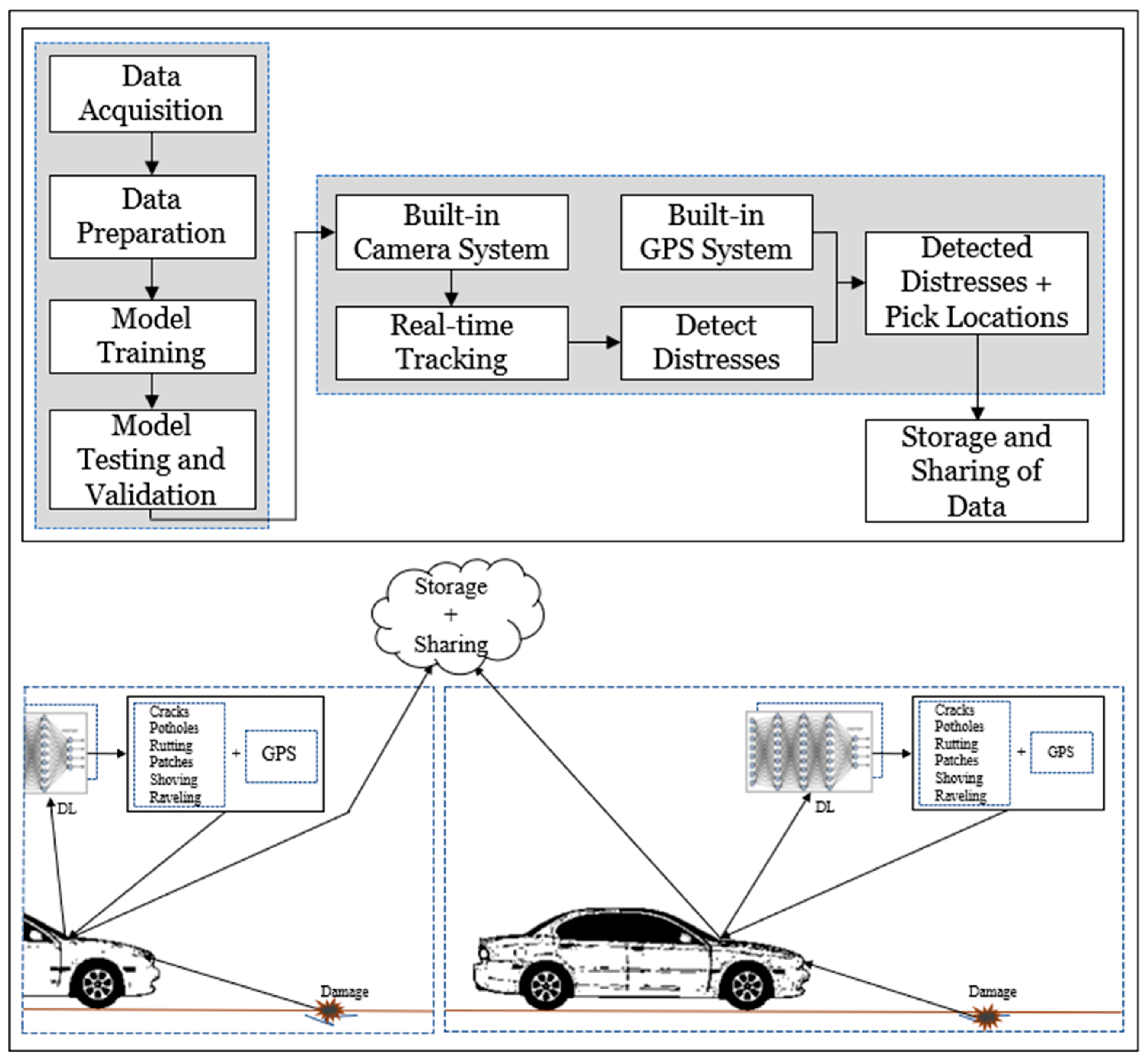
We propose an approach presented in Figure 1. A deep learning model is prepared, based on normal two-dimensional images, to detect and classify pavement damages/distresses into nine classes. The prepared model employs a vehicle-built-in camera to collect data on a real-time basis, and in connection to the built-in GPS sensors, the distresses are recorded with their corresponding geolocations. The recorded data are stored and shared on a real-time basis.

3.1. Model Selection

This study uses the You Only Look Once Version 5 (YOLOv5) model. This model was selected based on its advantages over its predecessors such as ease of use, ease of exporting to other file formats, small memory requirements of nearly 88% compared to YOLOv4 (27 MB vs. 244 MB), high speed (about 180% faster than YOLOv4, 140 FPS vs. 50 FPS), and its high accuracy value [42].

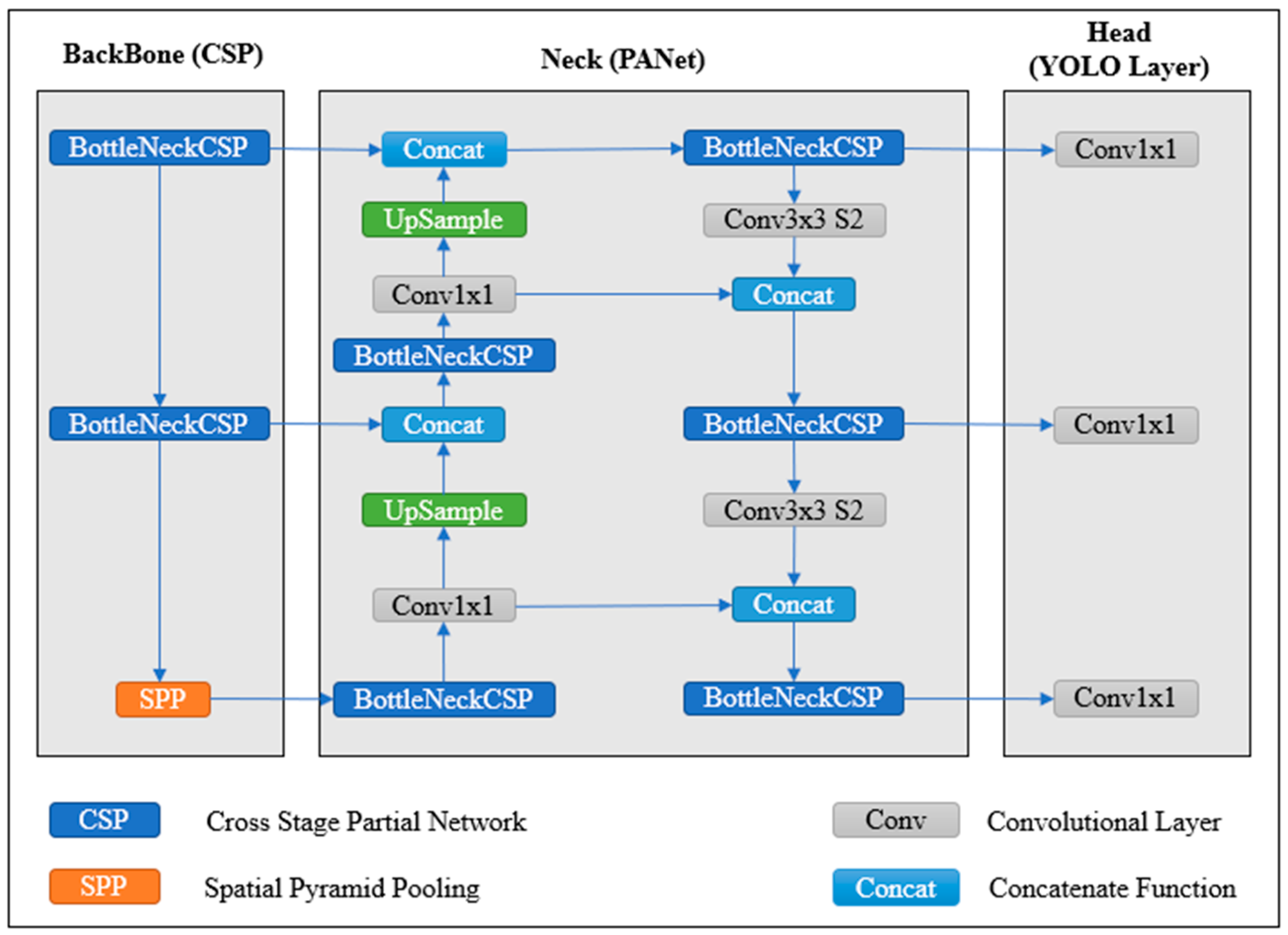
3.2. Model Structure

The architecture of the YOLOv5 network is presented in Figure 2. The network consists of 24 convolutional layers that extract features from the input data and then use these features to perform object detection using a set of head layers. The initial layers of this model are designed to detect low-level image features such as edges and shapes, and the filters become more complex and specialized as the layers progress to see more complex features. The network is divided into three main parts: backbone, neck, and head.

The head layers are divided into the neck and the detection head. The neck contains two convolutional layers that refine the features generated by the backbone layers. The output of the neck is used by the head layers to carry out prediction. The final classification head takes the detection head’s output and predicts the class. This output allows the network to detect multiple objects in images and classify them into different classes. The final predictions are stored in the output layer, including the bounding box coordinates, abjectness scores, and class probabilities.

3.3. Data Collection

This study used publicly available and onsite collected images and video datasets in model preparation, testing, and validation. The image datasets include the CRACK500 dataset collected at Temple University in Philadelphia using mobile phones [43]. RDD2020, an image dataset for smartphone-based road damage detection and classification, contains 26,336 smartphone images collected using smartphones mounted on car dashboards in India, Japan, and the Czech Republic ((accessible through the link: http://dx.doi.org/10.17632/5ty2wb6gvg), accessed on 20 May 2022)and another of pavement distresses v12-v4 from Roboflow which contains 665 images ((accessible through the link: https://public.roboflow.com/object-detection/pothole), accessed on 22 May 2022)). The video dataset was collected from American Honda Motor Co., Inc. (Torrance, CA, USA) [44] and it is made available upon request and upon signing of an agreement on the terms of use. In conducting model validation, some data were collected directly from the site within the campus.

The image dataset comprised normal two-dimensional (2D), colored images (RGB) with varying dimensions and shapes. The images were in a joint photographic experts group (JPG or JPEG) format, which is accepted by the selected model for training, validation, and testing purposes. The video dataset from Honda comprises about 84 h of real human driving scenarios collected from various roads in the state of California, U.S. All videos, including those recorded from campus, are in MP4 format.

3.4. Dataset Selection

A random sample of images was selected from the image datasets with a focus to represent all distress categories for training the model. This was accomplished by assigning names to all the images in the above-mentioned datasets using an Excel spreadsheet. Then randomization was performed by assigning random numbers generated in an Excel spreadsheet and a set of 8470 was selected for annotations.

The video dataset was analyzed, and some videos were selected in a focus to represent all ranges of driving speeds from 0 mph to 120 mph. The selection also took into consideration the different types of roads to be sure all types were represented. The types include arterial roads, collector roads, and local roads (access roads).

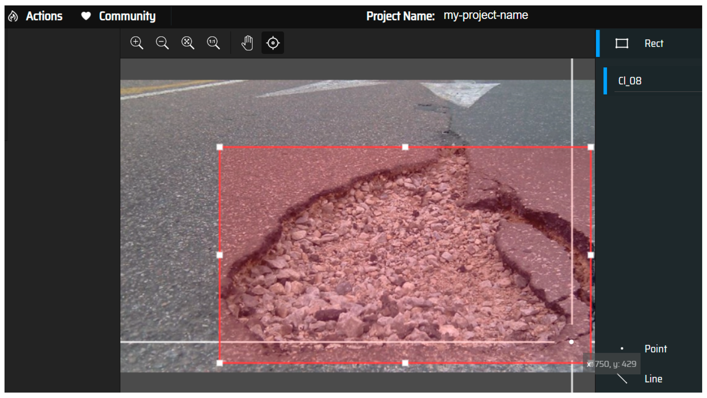
3.5. Dataset Preparation (Annotations)

Images for model preparation were annotated in YOLO format. The annotation process was performed using the makesense.ai [45] tool, which is freely available online. In this research, nine labels presented in

Table 1. Flexible distress classification as per U.S.DOT FHWA.

S/N	Class	Symbol Used
1	Fatigue/Alligator Cracks	Cl_01
2	Block Cracks	Cl_02
3	Transverse Cracks	Cl_03
4	Longitudinal—Wheel Path Cracks	Cl_04
5	Longitudinal—Non-Wheel Path Cracks	Cl_05
6	Edge, Joint, Reflective Cracks	Cl_06
7	Patches	Cl_07
8	Potholes	Cl_08
9	Raveling, Shoving, Rutting	Cl_09

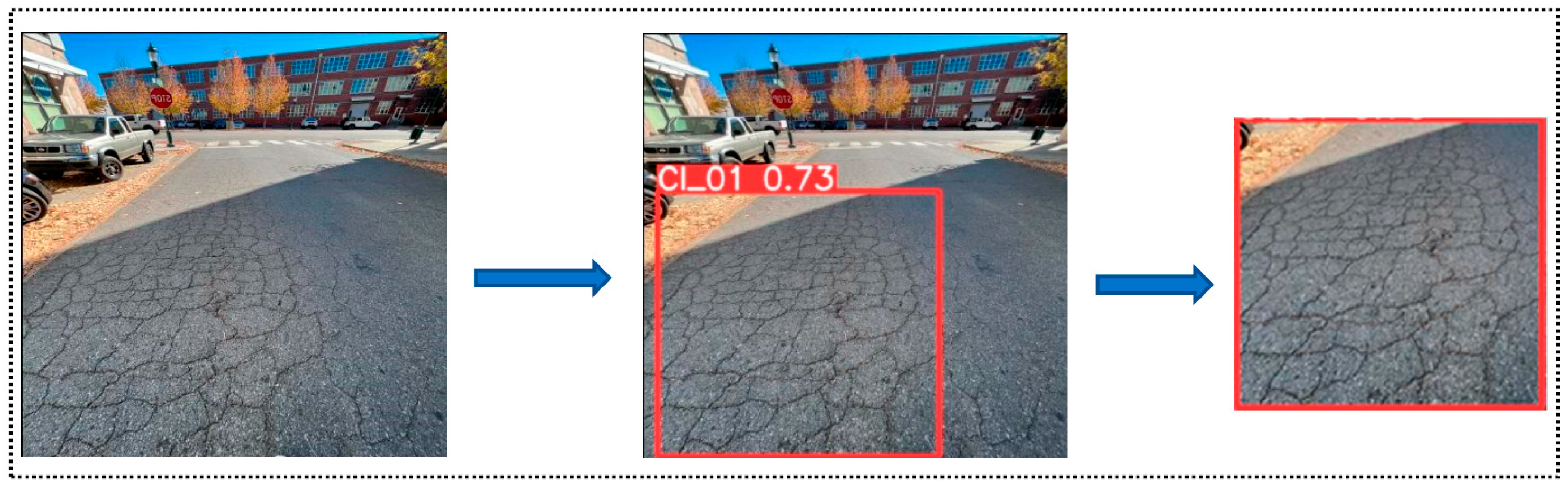
were assigned to the distresses at this point. Figure 3 below shows how the labels are assigned to the images.

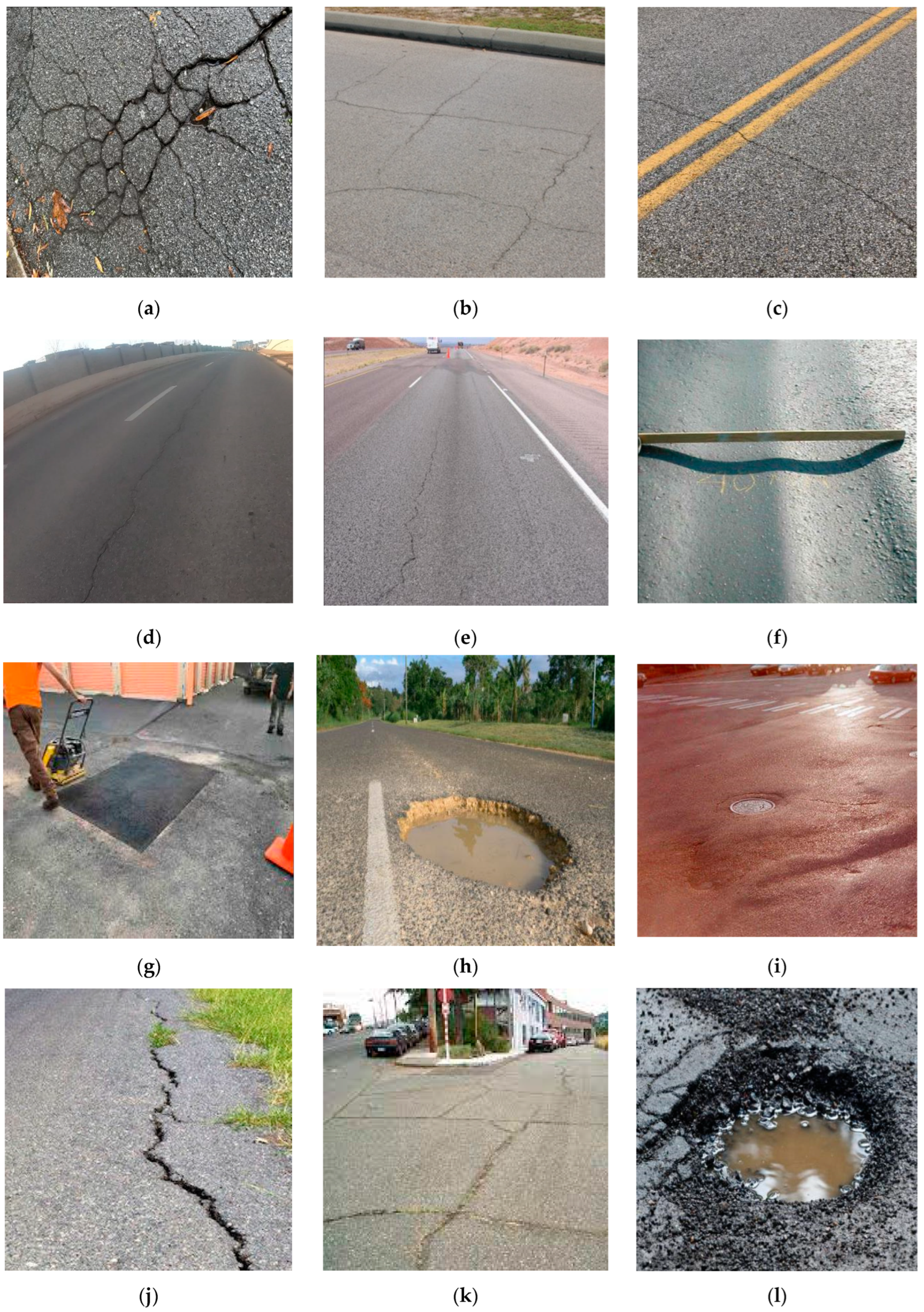
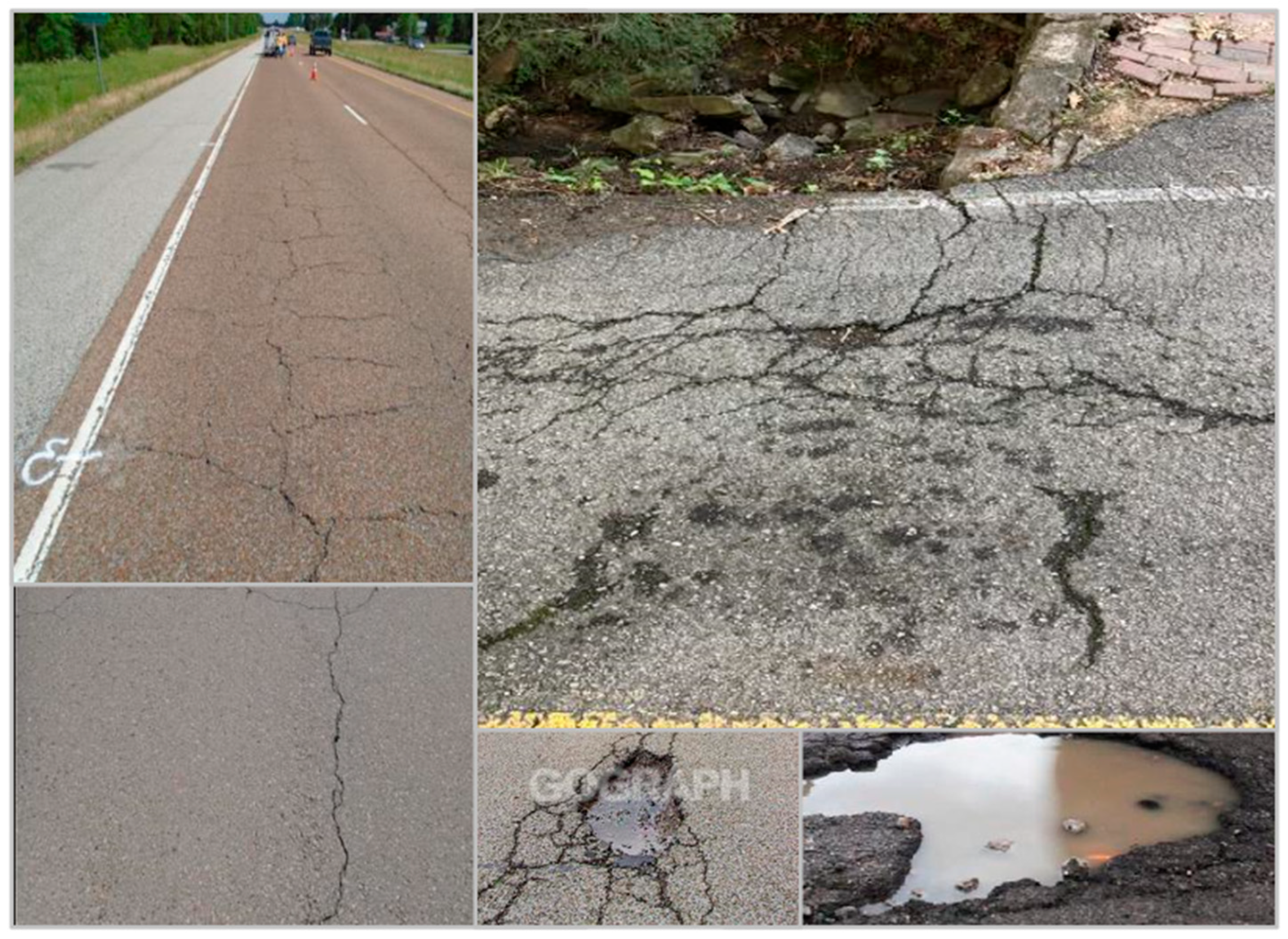
In this paper, a total of nine labels were assigned to images to represent the nine groups/categories of distresses and were exported in YOLO format. The assigned labels are included in text file formats, where a single file is formed for every image. Figure 4 illustrates some distress types, and the corresponding symbols used in representing them during labeling are shown in Table 1.

To reduce model overfitting and underfitting, it is necessary to provide more robust datasets so that the model becomes less reliant on similar pieces of data in the network [46]. Since some of the pavement distresses have a small number of instances, we decided to group them into the same classes; thus class 06 includes edge, joint, and reflective cracks, and class 09 includes raveling, shoving, and rutting.

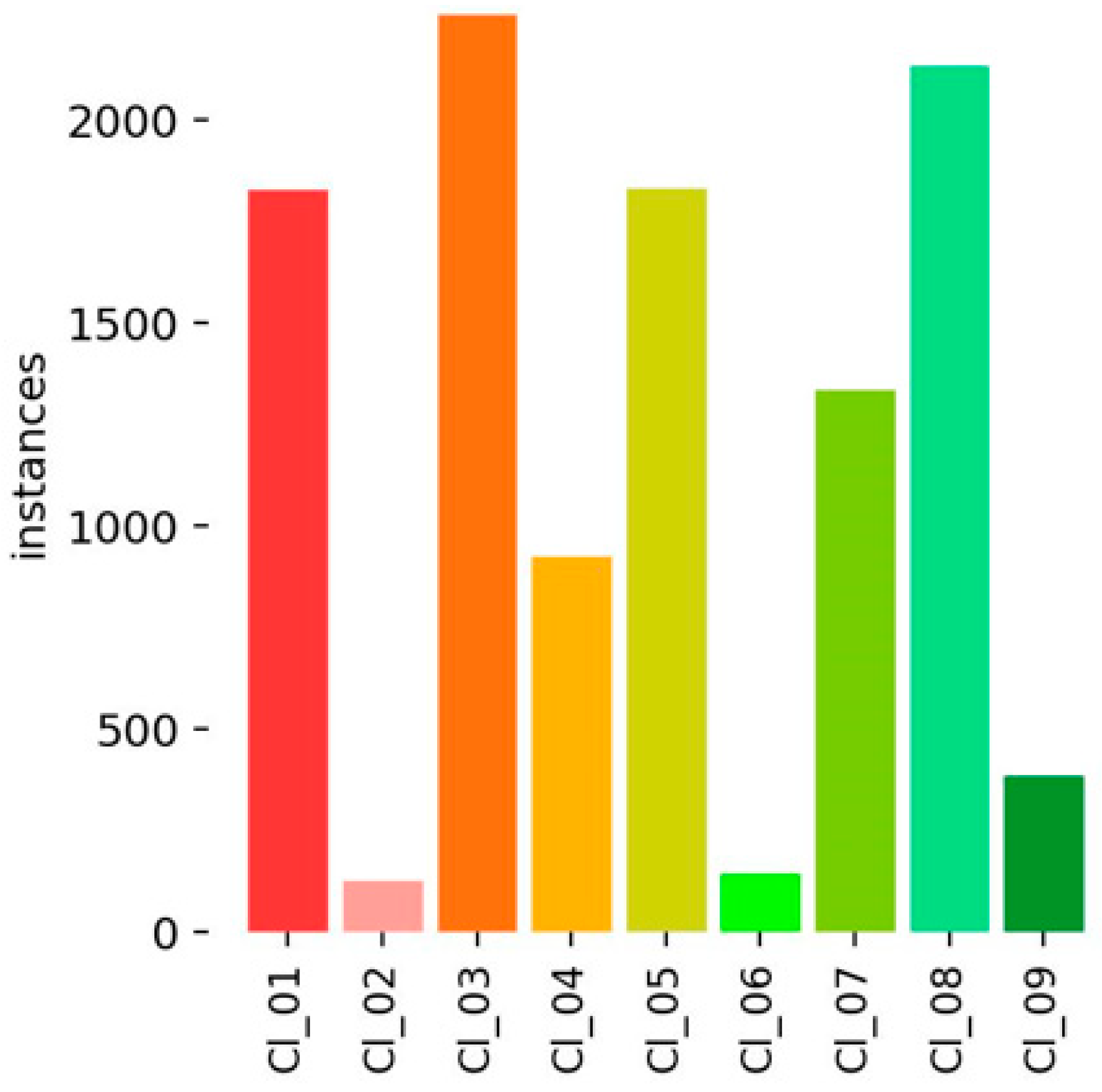
Figure 5 shows the number of instances (total number of repetitions/occurrences for each distress group). The Cl_03 class (transverse cracks) is the most represented class, with more than 2300 occurrences and the Cl_02 (block cracks) is the least represented class with less than 250 occurrences. The distribution trend depends on real-life scenarios where the most represented distress classes are much more common compared to those which are least represented. This is in line with a statistical study conducted in China to examine the relationship among asphalt concrete distresses, where findings show that some distresses which occur are independent distress types (IDDTs), dependent distress types (DDTs), and rutting secondary distress types (RSDTs). Results showed that RSDT (which was composed of bump, bleeding, roughness, and poor skid resistance) had the least occurrence probabilities, followed by DDTs (composed of longitudinal cracking, pumping, depression, and raveling). The IDDTs class (composed of transverse cracking, map cracking, potholes, and rutting) showed the highest occurrence probabilities [47].

3.6. Data Augmentation

An augmentation process is a procedure of changing the existing data to generate more data for the model to train on. It is performed only on the training dataset. Augmentation helps to avoid overfitting by increasing the available dataset through the application of various techniques [48] since detection models need a large amount of data to be efficient [49]. The techniques used in this study are rescaling, color adjustments, rotation, and mosaic augmentation.

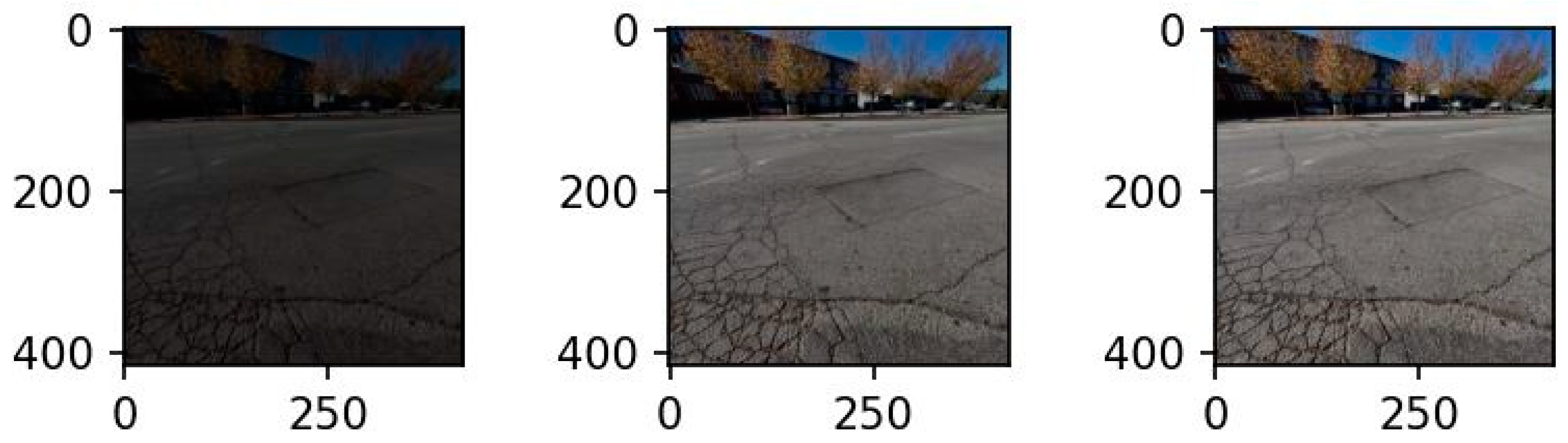
3.6.1. Rescaling

Rescaling involves increasing and decreasing an image size randomly by applying some random scaling factors. In this method, new images are generated without altering the objects, thereby increasing the size of the dataset. Figure 6 below shows an example of images formed from a single image by applying a rescaling factor of 75/255.

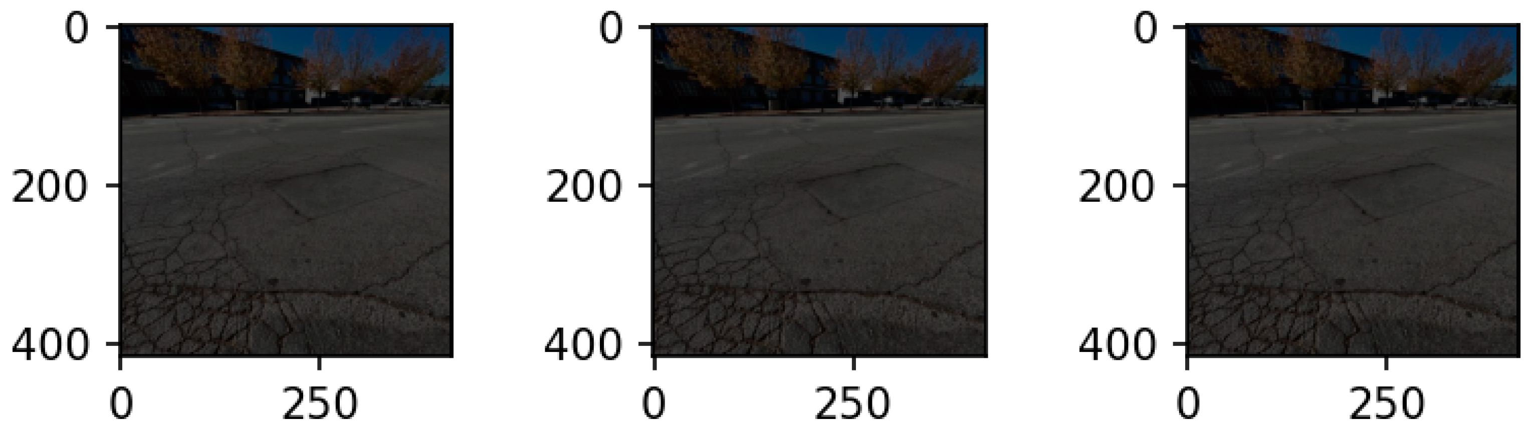
3.6.2. Color Adjustments

This involves changing the colors of the images. It can be accomplished by changing four aspects of the image color, namely, brightness, contrast, saturation, and hue. By assigning different values for these aspects, more images are generated; hence, the size of the dataset is increased. In Figure 7 below, brightness was randomly varied to obtain three different images.

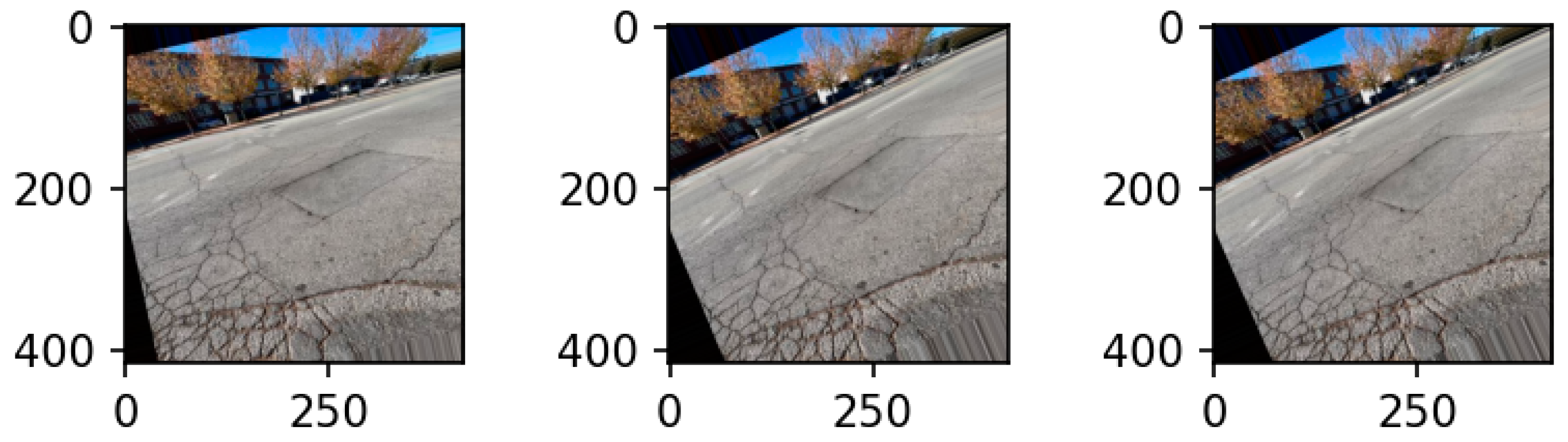
3.6.3. Rotation

Through rotations of an original image, other images are generated without affecting the identity of the objects of interest. The application of different rotation angles produces different images which are used to increase the size of the training dataset. Figure 8 shows an example of a rotation technique used in this paper.

3.6.4. Mosaic Augmentation

The mosaic data augmentation technique joins four training images into one in given ratios. This allows for the trained model to learn how to identify various objects at a smaller scale than normal, thereby increasing its performance. An example of mosaic augmentation is shown in Figure 9, which was formed during the model training process.

3.7. Model Training

In this study, the model was trained on Google Colaboratory (Google Colab). Before training, the dataset was split into two sets, one consisting of 80% of all images and another with the remaining 20%. The two sets were used for model training and validation, respectively.

An additional set of 200 images without distresses or labels were used as background images to reduce the effect of False Positives (FPs) and False Negative (FNs) and hence increase our model’s accuracy. This set was included in the training set only.

3.8. Training Parameters

To attain desirable results, the model was trained at different parameter settings. Starting with a default image size of 416 pixels, different values of batch sizes and numbers of epochs were fed.

Table 2. Training parameters.

S/N	Parameter	Value
1.	Batch Size	40
2.	Epochs	150
3.	Learning Rate	0.01
4.	Optimizer	SGD = 0.01
5.	Anchor Sizes	Dynamic

shows the final values of parameters used in training the model. The training was completed in 3.216 h.

3.9. Model Analysis and Evaluation

The analysis and the evaluation of Deep Learning models are achieved through the assessment of performance metrics. These values are obtained at the end of the validation or testing that is performed when training is completed. The performance metrics used are precision, recall, and mean average precision (mAP). Precision measures the model’s accuracy in correctly predicting the distress, whereas recall measures the model’s performance in finding all distresses in the images (it is a function of how the model misses the distresses). Precision and recall are functions of False Positives (FPs) and False Negative (FNs), which are also regarded as type I and type II errors, respectively. The FPs are the measures that show how the model incorrectly predicts pavement distresses, whereas the FNs show how the model misses them. Precision and recall values are calculated as the ratios of TPs to the sum of TPs, FPs, and FNs as shown in Equations (1) and (2), respectively.

$$\mathrm{P}\mathrm{r}\mathrm{e}\mathrm{c}\mathrm{i}\mathrm{s}\mathrm{i}\mathrm{o}\mathrm{n}=\frac{\mathrm{T}\mathrm{r}\mathrm{u}\mathrm{e} \mathrm{P}\mathrm{o}\mathrm{s}\mathrm{i}\mathrm{t}\mathrm{i}\mathrm{v}\mathrm{e}\mathrm{s}}{\mathrm{T}\mathrm{r}\mathrm{u}\mathrm{e}\mathrm{ }\mathrm{P}\mathrm{o}\mathrm{s}\mathrm{i}\mathrm{t}\mathrm{i}\mathrm{v}\mathrm{e}\mathrm{s} + \mathrm{F}\mathrm{a}\mathrm{l}\mathrm{s}\mathrm{e} \mathrm{P}\mathrm{o}\mathrm{s}\mathrm{i}\mathrm{t}\mathrm{i}\mathrm{v}\mathrm{e}\mathrm{s}}$$

(1)

$$\mathrm{R}\mathrm{e}\mathrm{c}\mathrm{a}\mathrm{l}\mathrm{l}=\frac{\mathrm{T}\mathrm{r}\mathrm{u}\mathrm{e} \mathrm{P}\mathrm{o}\mathrm{s}\mathrm{i}\mathrm{t}\mathrm{i}\mathrm{v}\mathrm{e}\mathrm{s}}{\mathrm{T}\mathrm{r}\mathrm{u}\mathrm{e}\mathrm{ }\mathrm{P}\mathrm{o}\mathrm{s}\mathrm{i}\mathrm{t}\mathrm{i}\mathrm{v}\mathrm{e}\mathrm{s} + \mathrm{F}\mathrm{a}\mathrm{l}\mathrm{s}\mathrm{e} \mathrm{N}\mathrm{e}\mathrm{g}\mathrm{a}\mathrm{t}\mathrm{i}\mathrm{v}\mathrm{e}\mathrm{s}}$$

(2)

The mAP is the mean (average) of average precisions of all individual classes in the model. It is calculated as the sum of the average precisions of all individual classes divided by the total number of classes as shown in Equation (3) below.

$$\mathrm{mean} \mathrm{Aaverage} \mathrm{Precision}\left(mAP\right)=\frac{1}{n}\sum _{k=1}^{k=n}{AP}_k$$

(3)

where ${AP}_k$ stands for the average precision of class k, and n stands for the total number of classes.

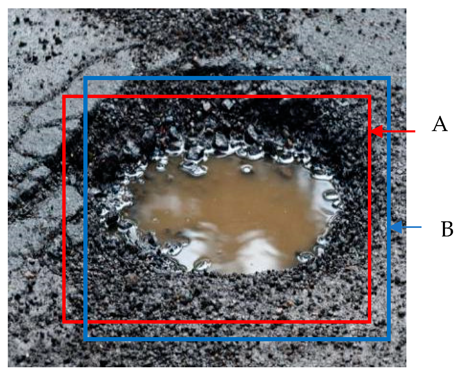
These performance metrics are directly affected by the Intersection over Union (IoU), which is the measure of the areas formed on the images between the ground truth bounding boxes (actual bounding boxes) and the predicted bounding boxes. Intersection refers to the area covered by both bounding boxes, whereas union refers to the total area covered by the two bounding boxes. Figure 10 shows an illustration of the IoU given by Equation (4).

$$\mathrm{I}\mathrm{o}\mathrm{U}=\frac{\mathrm{Area}\left|A\cap B\right|}{\mathrm{Area}\left|A\cup B\right|}$$

(4)

The value of IoU obtained using the above relationship determines whether the output is TP or FP. The output becomes TP if the value is greater than or equal to the threshold value (which was set to 0.45 in our model), and it becomes FP if the value is less than the threshold value [50].

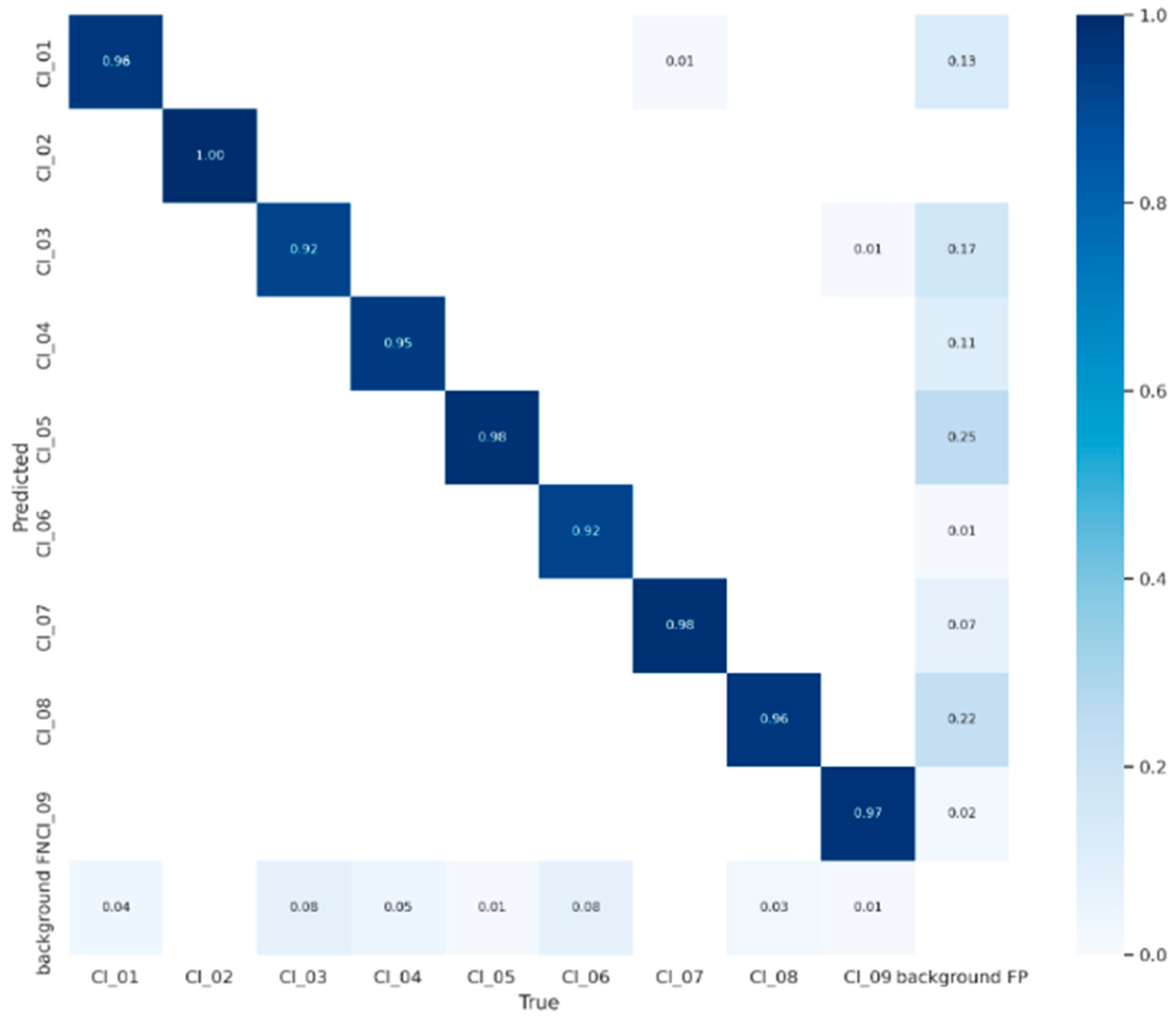
Figure 11 shows a confusion matrix indicating the resulting relationship between the True Positives, True Negatives, False Positives, and False Negatives. Having values that are close to or equal to 1 along the diagonal indicates that the model has high values of precision and recall.

3.10. Model Testing

3.10.1. Model Testing on Still Images

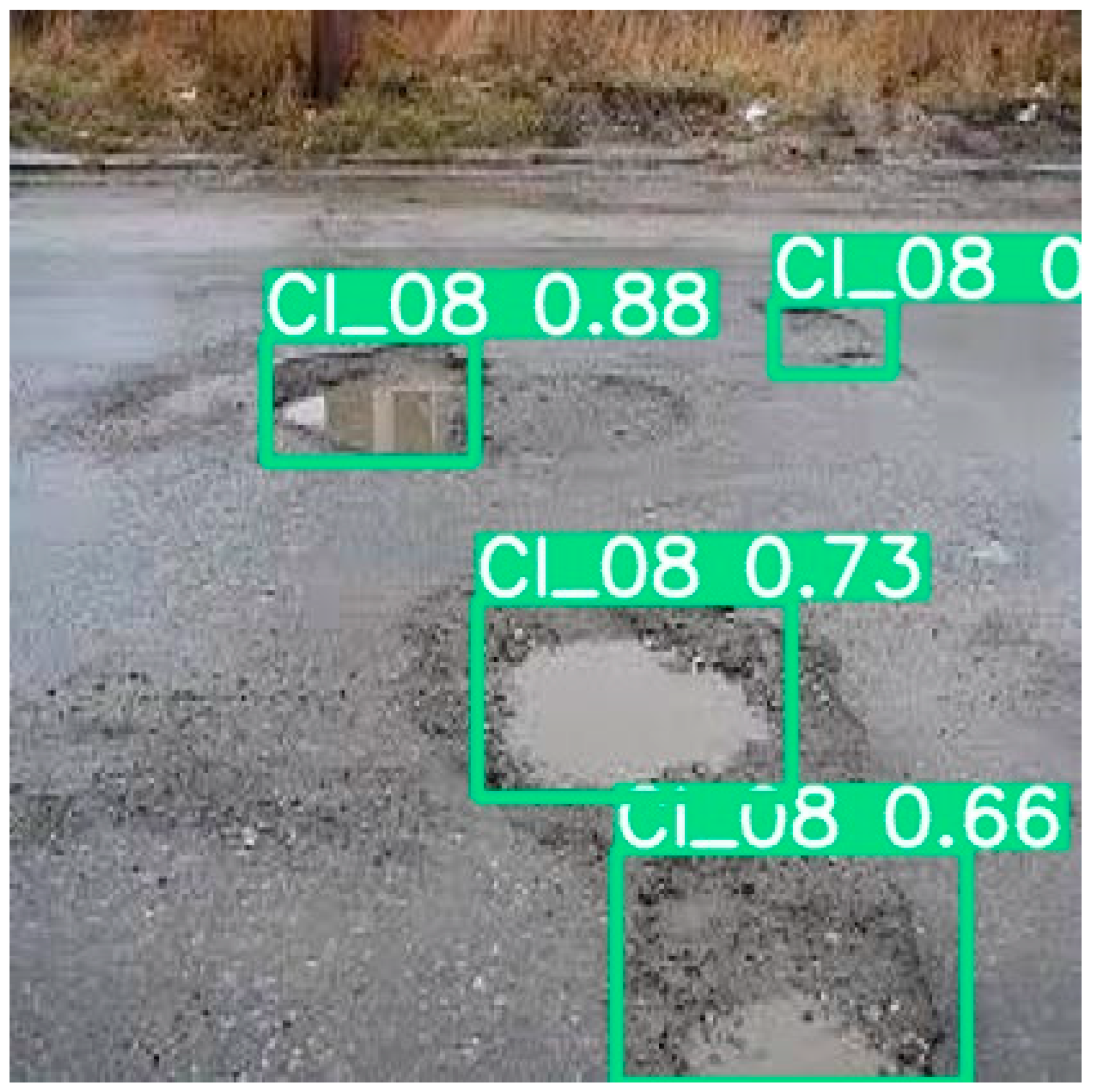
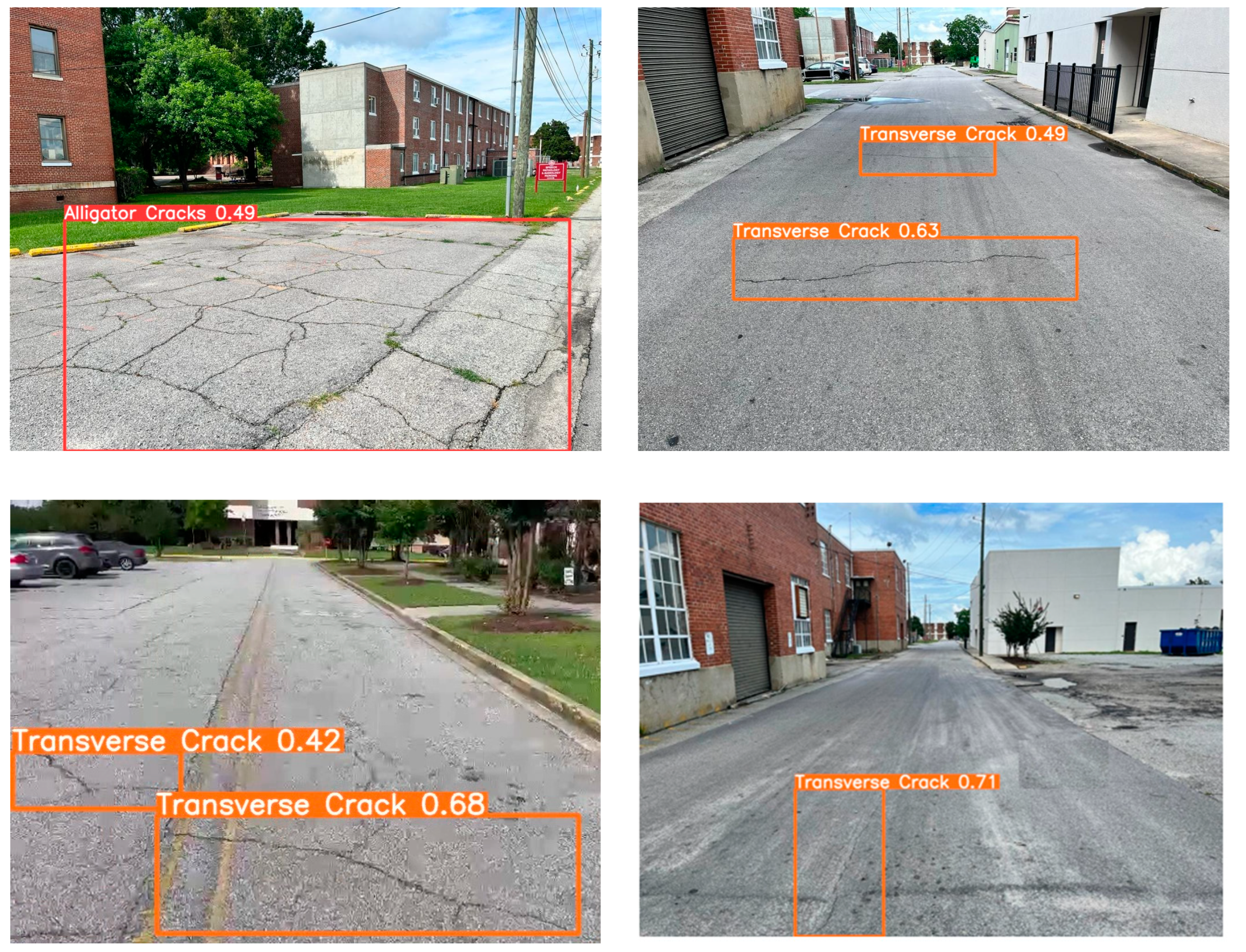
The model attained 95%, 93.4%, and 97.2% overall average values in precision, recall, and mean Average Precision at 50% (mAP@.5), respectively. The ability of the model to predict pavement distresses was also assessed on both still images and videos. Testing of the model on videos aimed at mimicking its performance on the videos from vehicles’ built-in cameras. Figure 12 shows the sample prediction results with distress symbols and their respective prediction confidences obtained for various pavement distress classes, and

Table 3. Summary of the model test results on still images.

S/N	Class	Precision (%)	Recall (%)	mAP@.5
1	Cl_01	94.9	93.7	97.6
2	Cl_02	97.9	100.0	99.5
3	Cl_03	94.1	83.5	93.9
4	Cl_04	91.6	93.7	95.6
5	Cl_05	93.1	94.3	97.4
6	Cl_06	97.4	92.3	96.2
7	Cl_07	95.6	98.3	99.3
8	Cl_08	93.0	91.6	96.3
9	Cl_09	97.2	93.3	98.7

shows the summary of results on still images.

3.10.2. Model Testing on Videos at Different Driving Speeds

To assess the performance of the model at different driving speeds, a total of eighty-one video clips were assessed. The clips were grouped into six-speed groups, namely, 0–20 mph, 20–40 mph, 40–60 mph, 60–80 mph, 80–100 mph, and 100–120 mph. For each speed group, the clips were passed through the model for detection of distresses and then used to generate frames from which the detections were assessed.

Table 4. The summary of video analysis results.

S/N	Speed (Mph)	Precision (%)	Recall (%)
1.	0–20	67	90
2.	20–40	57	86
3.	40–60	59	62
4.	60–80	54	88
5.	80–100	65	76
6.	100–120	66	87

shows the summary of precision and recall values obtained for each speed group.

To improve these results, the model was re-trained. This time, the albumentation library was installed and augmentation parameters were fine-tuned to improve the dataset before training. The parameters adopted include Blur (blur_limit = 50, p = 0.05), Median blur (blur_limit = 50, p = 0.02), ToGray (p = 0.3), CLAHE (p = 0.02), Random Brightness Contrast (p = 0.2), RandomGamma (p = 0.2), and ImageCompression (quality_lower = 75, p = 0.2). In these parameters, p stands for probability. Fine-tuning these parameters improved the model results on the videos for all speed ranges.

Table 5. Summary of video analysis results after fine-tuning the augmentation parameters.

S/N	Speed (Mph)	Precision (%)	% Improvement in Precision	Recall (%)	% Improvement in Recall
1.	0–20	78	11	95	5
2.	20–40	81	24	94	8
3.	40–60	76	17	92	30
4.	60–80	85	31	93	5
5.	80–100	79	14	86	10
6.	100–120	82	16	91	4

shows the summary of video analysis results after fine-tuning.

4. Discussion of Testing Results

Table 3 summarizes the results of the testing of the trained model on still images. These results show that the model attained a precision of more than 93.0% for all classes, a recall of more than 91.6%, and a mAP@50% of more than 93.9%. These values mean that the model achieved satisfactory results in predictions and had small numbers of False Positives and False Negatives. These results are comparable to the state-of-the-art of currently published studies such as the research by Maeda et al. (2018) who worked to classify pavement distresses using SSD Inception V2 and SSD MobileNet frameworks and achieved recalls and precision greater than 71% and 77% and overall accuracy of 87.75% and 87.25%, respectively.

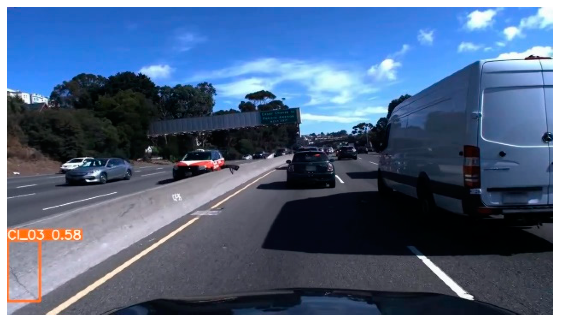
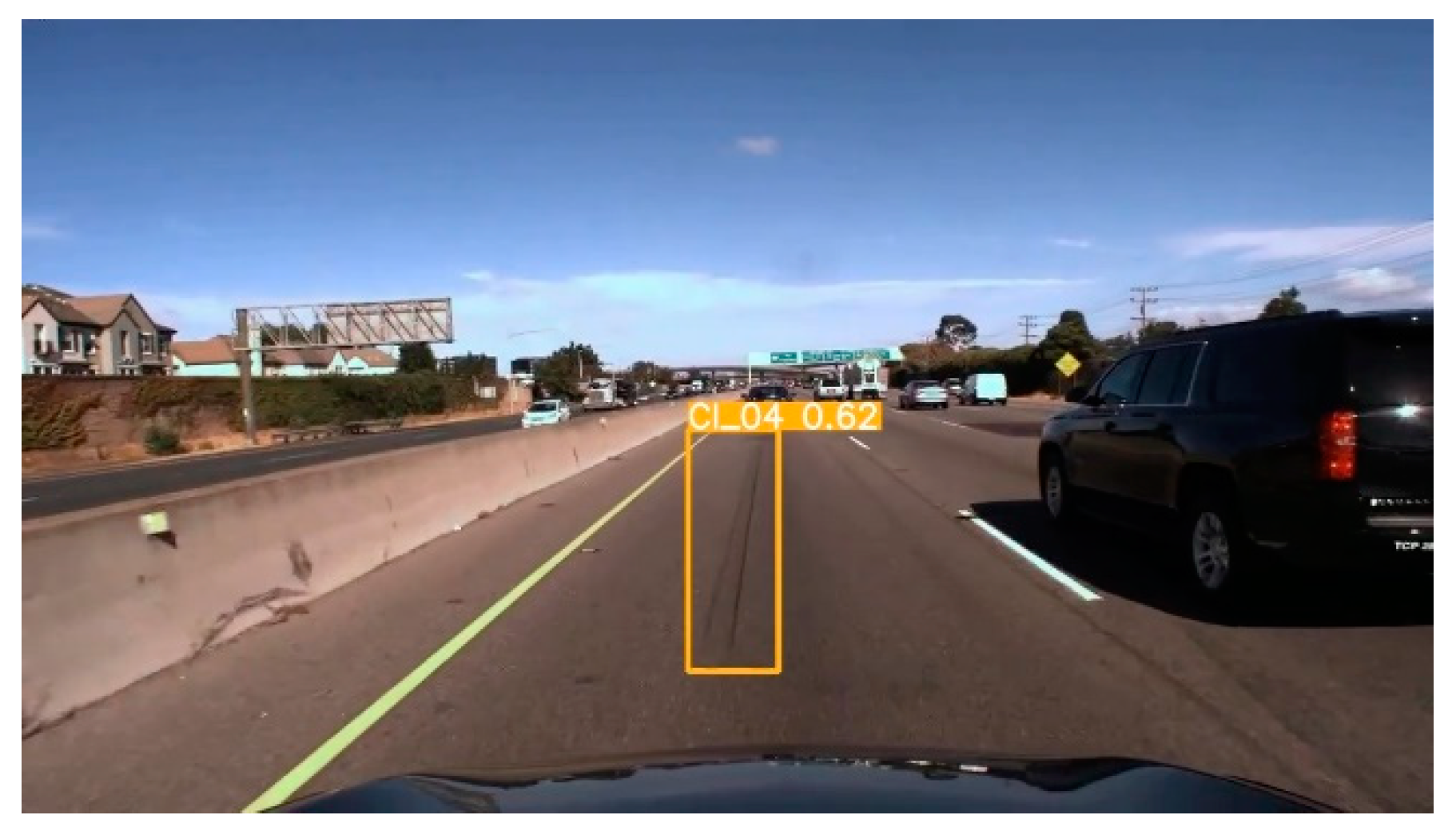
Table 4 shows the video analysis results. These results are attributed to some common errors in the detection, such as the inclusion of cracks on barrier walls (Figure 13) and skid marks (Figure 14), among others. Due to this, we found it necessary to re-train the model to improve its accuracy.

Table 5 summarizes the final testing results on videos at different driving speeds. Tuning the parameters helped the model skip the distresses on barrier walls, and skid marks were not confused with the distresses. This resulted in increased values in both precision and recall at all speed ranges, since a smaller number of errors were encountered.

The results show that the model performance is not much influenced by the driving speed since high accuracy values are obtained at all speed ranges. Therefore, the model can be used to detect distresses at any driving speed with high accuracy. This indicates that the model can be used to detect pavement distresses using vehicle built-in cameras, which is the primary objective of this study.

4.1. Detection, Taking Photos, and Geolocations

When a vehicle camera is used, pavement distresses on road surfaces will be detected and rectangular bounding boxes will be drawn around them, with colors and symbols to represent the classes of detected distresses. These bounding boxes are increased by 20 pixels on all sides to provide a buffer and avoid overtight, and corresponding detections are saved as independent images (see Figure 15). While in motion, the vehicles record Global Positioning System (GPS) tracks (using built-in GPS sensors) in parallel with the distress detections by the built-in camera. At the end of the trip, the recorded GPS track can be used to obtain the coordinates of locations where distresses were detected and recorded.

4.2. Model Validation

The model was validated within South Carolina State University campus using a car. The car is equipped with a built-in camera and GPS sensors, the features of interest for our study. The vehicle was driven on about 1.5 miles of roadway and parking lots, and we collected 53 images with various distress types, some of which are presented in Figure 16.

5. Conclusions

This paper used YOLOv5 to train the model to detect and classify pavement distress conditions. The image data used were collected from different countries, with different devices, and have different properties as various methodologies have been employed in pavement construction and rehabilitation. All the images were raw and therefore manual labeling was performed using the makesense.ai tool. To increase the dataset size, image augmentation was performed before training, and background images were included in the training dataset to reduce the FPs. The trained model attained 95%, 93.4%, 84.6%, and 97.2% values in precision, recall, F1-score, and mean average precision at 50% (mAP@.5), respectively.

The model was also tested on videos taken at different driving speeds from 0 mph to 120 mph. The results obtained show high accuracy values at all speed levels (up to 85% precision and 95% recall). With these results, the model was able to detect and classify the distresses into their respective classes. Once recorded, the distresses can be analyzed parallel to the GPS file; therefore, the type and location of the distress can be obtained for further actions. The performance of the proposed model was verified on campus roads and proved to be effective.

6. Limitations and Future Recommendations

This study proposes using vehicle cameras to collect road damage data, a process whose effectiveness is greatly affected by light illumination intensity. If this approach is employed during night-times/poor illumination conditions, we recommend the use of proper headlights or appropriate light technologies to improve performance. Also, this study is limited to the detection and classification of pavement damage. Future studies may improve the study by incorporating severity classification, where the detected distresses may be further classified based on the extent of deterioration.