A Refined-Line-Based Method to Estimate Vanishing Points for Vision-Based Autonomous Vehicles

Abstract

Helping vehicles estimate vanishing points (VPs) in traffic environments has considerable value in the field of autonomous driving. It has multiple unaddressed issues such as refining extracted lines and removing spurious VP candidates, which suffers from low accuracy and high computational cost in a complex traffic environment. To address these two issues, we present in this study a new model to estimate VPs from a monocular camera. Lines that belong to structured configuration and orientation are refined. At that point, it is possible to estimate VPs through extracting their corresponding vanishing candidates through optimal estimation. The algorithm requires no prior training and it has better robustness to color and illumination on the base of geometric inferences. Through comparing estimated VPs to the ground truth, the percentage of pixel errors were evaluated. The results proved that the methodology is successful in estimating VPs, meeting the requirements for vision-based autonomous vehicles.

1. Introduction

Robust VP estimation has considerable value in vision-based navigation for autonomous vehicles. Due to the diversity of traffic environments, there are a multitude of disturbances caused by clutter and occlusion, resulting in multiple challenges in line segments refinement and spurious vanishing candidate removal. Therefore, estimating VPs, especially in complex surroundings, remains a challenge for vision-based autonomous vehicles.

For a monocular camera, how can a vision-based autonomous vehicle extract valuable textures and describe their features that can be interpreted in upper inferences such as environmental perception? The perception of depth in the human visual system requires no additional knowledge [1]. The geometric jointed points are more like to be used in approximating relative depth of different features [2]. Accordingly, it can be assumed that some structured rules can be used to approximate those geometric VPs [3], and the accurate estimation of VPs is the cornerstone in understanding a scene [4,5]. However, complex surroundings make existing methods suffer greatly from low accuracy and high computational cost because of disturbance from a great deal of extracted line segments. Therefore, to efficiently estimate VPs is increasingly playing a vital role in visual navigation of autonomous vehicles.

In this study, we present an approach to estimate VPs from a monocular camera with no prior training and no internal calibration of the camera. The main contributions of this paper are as follows:

• a method designed to effectively refine lines that satisfy structured shape and orientation;
• an algorithm developed to remove spurious VP candidates and obtain the VP by optimal estimation;
• an approach presented to estimate the VPs through refined-line strategy, which is robust to varying illumination and color.

Unlike existing approaches, using basic line segments directly, the proposed method adopts a strategy based on refined lines that belong to structured configuration and orientation, which has a better robustness in the estimation process. Compared to data-driven methods, the proposed method requires no prior training. Simple geometric inferences endow the proposed algorithm with the ability to adapt to the image with changes in illumination and color, making it practical and efficient for scene understanding in autonomous vehicles.

Through evaluating the percentage of pixel errors from the ground truth, experimental results demonstrated that the proposed algorithm can successfully estimate VPs in a complex environment with low consumption and high efficiency, which has extremely broad application prospects for scene understanding and visual navigation in the future.

The structure of the paper is elucidated as following. Section 2 shows the relation work including estimation of vanishing point and its application in scene understanding. Section 3 indicates the model of refining lines and obtaining optimal vanishing point. Section 4 shows the results and comparison for the proposed method. In Section 5, we present a conclusion of the work.

2. Related Work

As to human visual system, a capture essentially is an optical signal from the environment. It was indicated that the optical signal is possible to be transformed into a neural signal in a retina [6]. For the sampling process in a retina, the photoreceptor, which is to alter an optical signal to a neural signal, appears with a nonuniform distribution [7]. An algorithm was introduced to simulate the sampling strategy by a iterative process and a distribution with different densities [8]. Edges of a capture are only a set of disorganized unorganized pixels, and visual cues can be represented, organized, and propagated by geometric constraints [9,10]. Compared to process original stimulus, a signal of stimuli is possible to be coded and transmitted in a refined strategy.

Classic algorithms of VPs estimation were introduced. An approach was presented to investigate VPs of stair region verification based on the three basic criteria [11]. To solve the tilting orientation angles, an online calibration algorithm was introduced to estimate camera orientation through motion vectors and three-dimensional geometry [12]. A method was proposed to improve the efficiency of the metaheuristic search for VPs through a population-based algorithm [13]. A VP detection method was presented to select robust candidates and clustering candidates by optimized minimum spanning tree and lines within a unit sphere domain [14]. A generic method based on VP was proposed to reconstruct the 3D shape of document pages without segmenting the text included in the documents [15]. A methodology was presented to improve VP detection in landscape images based on improved edge extraction process using combining different representations of an image [16]. An approach was proposed to estimate VPs using a harmony search (HS) algorithm [17]. A method was proposed to estimate VPs and camera orientation based on sequential Bayesian filtering [18]. These approaches have weak ability to obtain VPs in a traffic scene filled with clutter and occlusion.

Recently, many works have studied VPs in scene understanding and visual navigation. An algorithm was proposed to detect unstructured road VP by combining the convolutional neural network (CNN) and heatmap regression [19]. 3D interaction between objects and the spatial layout were built through prediction of VPs [20,21,22]. Another approach was proposed to infer wheelchair ramp scenes based on multiple spatial rectangles through domain VPs, but it requires a clean environment [23]. A regression approach was presented to detect the position of VPs with a residual neural network [24]. A method using geometric features to extract VPs was adopted to focus obstacle avoidance for a robot in an indoor environment [25,26]. A framework was presented for detecting stair region from a stair image utilizing some natural and unique property of a stair [27]. However, these algorithms have difficulty estimating VPs for road environments with complicated clutters and obstacles.

Impressive models were proposed in traffic environments. A method was proposed to detect VPs of unstructured road scenes in which there are no clear road markings in complex background interference [28]. A method was proposed to estimate VPs based on road boundaries region estimation by the line-soft-voting based on maximum weight [29]. A detection technique was proposed to detect VPs in complex environments such as railway and underground stations with variable external conditions for surveillance applications [30]. For street scenes, those curved buildings and handrails also can be understood in 3D reconstruction on the base of estimated VPs [31]. In order to settle the issue of lane keeping, a strategy was proposed to obtain instant control inputs through camera perception [32]. However, these methods are prone to failure in robust VP estimation due to varying disturbance in complex traffic environments.

Therefore, it becomes an urgent need to look for a kind of refined-line-based algorithm to estimate the VPs for vision-based autonomous vehicles from a monocular camera without prior training. Furthermore, a refined-line-based strategy for VP estimation with lower cost and higher efficiency was more practicable and feasible for scene understanding and visual navigation.

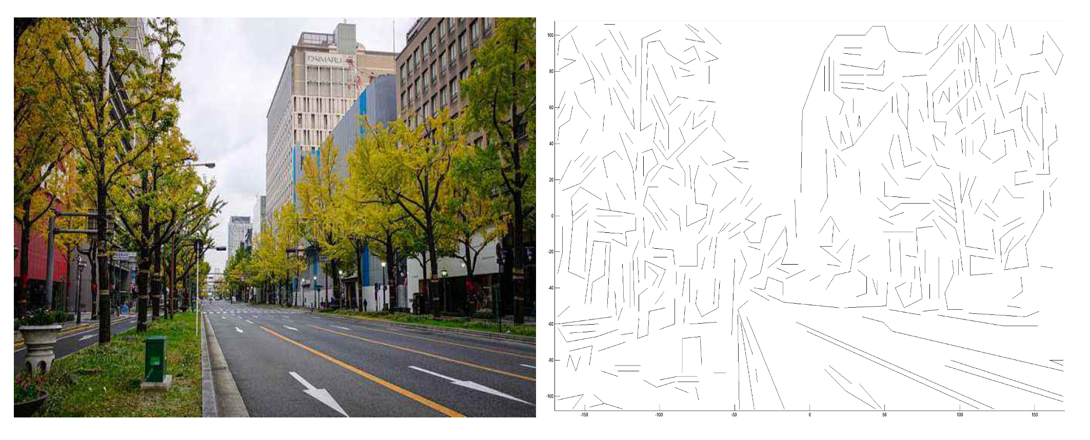
3. Vanishing Point Estimation

In a complex traffic environment, there are many diverse spatial corners whose spatial lines tend to be projected and detected. Some of them satisfy special geometric constraints. These spatial lines are projected into 2D angle projections that have diverse configurations. These special lines are of great importance in estimating their orientation and corresponding VPs in a such environment.

3.1. Preprocessing

Lines are extracted [33,34,35] as follows:

$$\begin{array}{c}\hfill \mathbb{L}=\left\{lin{e}_i\right\}=[x_1^i,y_1^i,x_2^i,y_2^i],i\in \mathbb{N}\end{array}$$

(1)

where $\mathbb{N}$ is the number of lines. $\mathbb{L}$ is a set of lines.

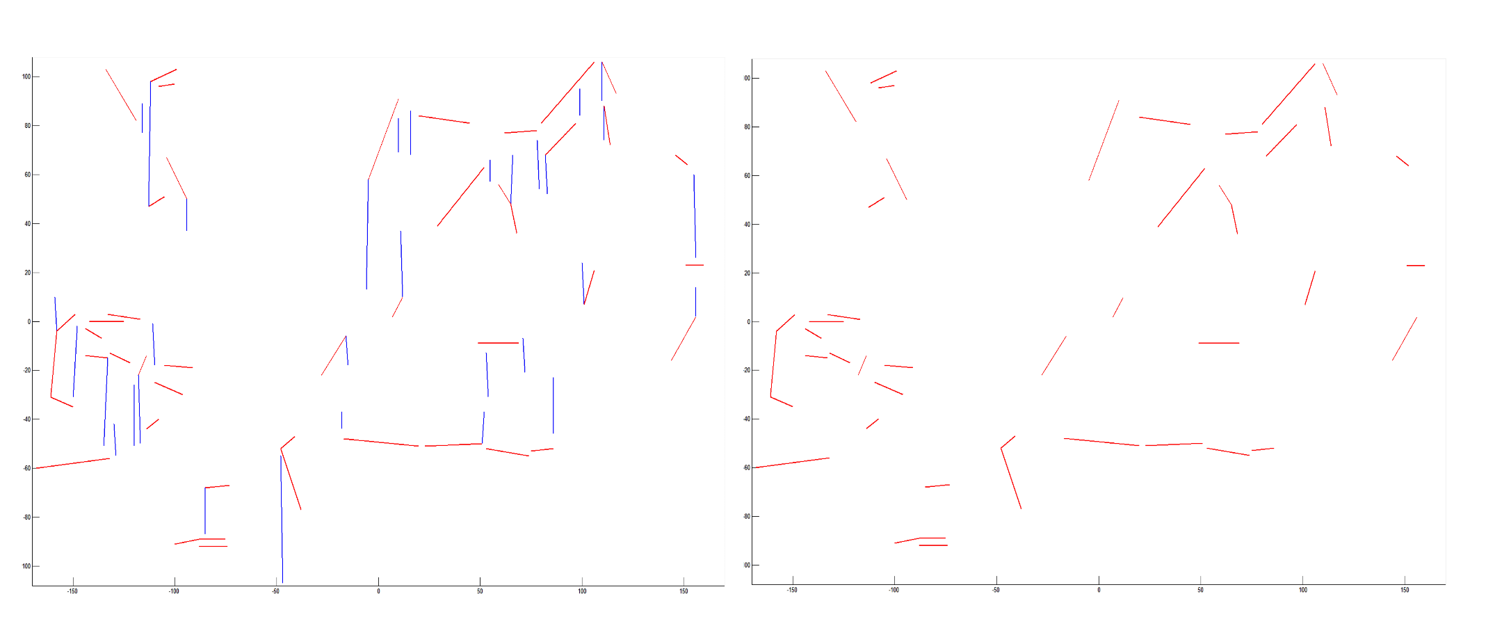
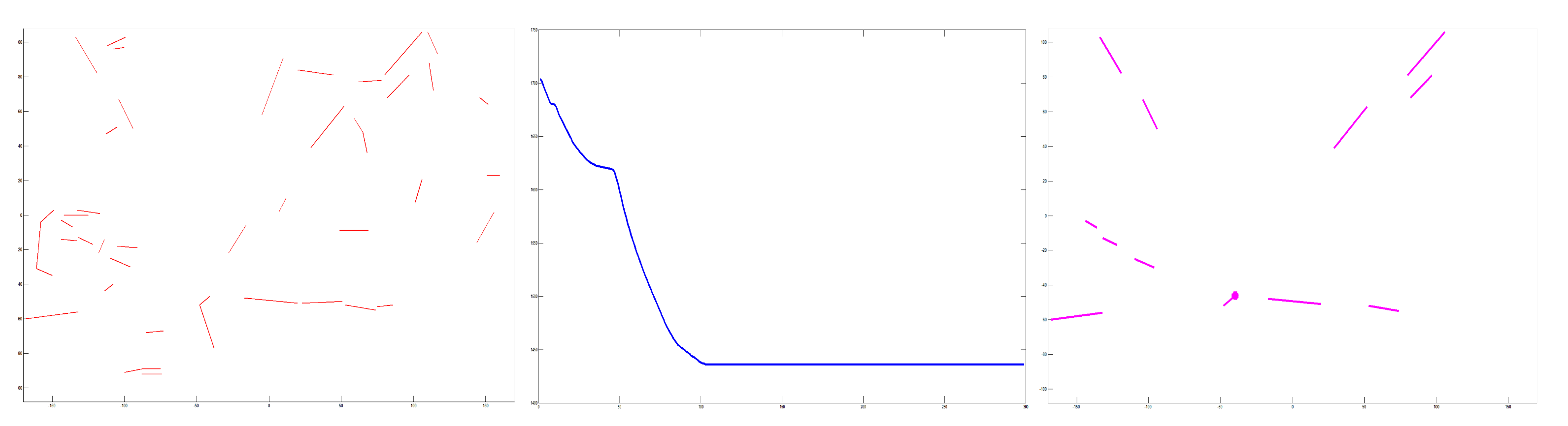
3.2. Refining Lines

Due to complexity of environment, there are multiple textures of diverse clutter and occlusion that project into a large number of lines, causing unavoidable disturbance and extremely high computational cost. To refine lines is the key to greatly enhance the efficiency of estimating VPs. Humans are always sensitive to those structured configurations. Compared to isolated lines, those lines that lie in structured configurations seem to be more valuable. Since accurate depth can not be determined from a single capture, the camera is arbitrarily positioned at the origin of the world coordinate system and pointing down the z-axis.

For $s,n\in \mathbb{N}$, then corresponding geometric constraints for these two lines can be defined as follows:

$$\begin{array}{cc}\hfill {\sigma }^s& =\parallel p_c-p_m^s{\parallel }_2-l^s/2;\hfill \end{array}$$

(2)

$$\begin{array}{cc}\hfill {\sigma }^n& =\parallel p_c-p_m^n{\parallel }_2-l^n/2;\hfill \end{array}$$

(3)

$$\begin{array}{cc}\hfill {\varsigma }^s& ={\theta }^s-\pi /2\hfill \end{array}$$

(4)

Here, $p_c$ is the intersection of two lines $lin{e}_s$ and $lin{e}_n$ in an angle projection. $p_m^s$ and $l^s$ are the midpoint and length related to $lin{e}_s$. $p_m^n$ and $l^n$ are the midpoint and length related to $lin{e}_n$. ${\sigma }^s$ represents geometric integrity for $lin{e}_s$, and ${\sigma }^n$ represents geometric integrity for $lin{e}_n$. ${\varsigma }^s$ means the geometric orientation constraints for $lin{e}_s$.

For all above obtained values, then the following can be found:’

$$\begin{array}{cc}\hfill {\mathrm{\Lambda }}^{s,n}& =\parallel {\sigma }^s{\parallel }_2+\parallel {\sigma }^n{\parallel }_2+{\parallel {\varsigma }^s\parallel }_2\hfill \end{array}$$

(5)

Here, ${\mathrm{\Lambda }}^{s,n}$ that are normalized represent the geometric constraints including both integrity and orientation for $lin{e}_s$ and $lin{e}_n$. The smaller value of ${\mathrm{\Lambda }}^{s,n}$ means that this composition of two lines $lin{e}_s$ and $lin{e}_n$ are more likely to be noticed.

In this way, the composition of two lines ($lin{e}_s$ and $lin{e}_n$) are both extracted. Accordingly, the cluster of refined lines are determined as follows:

$$\begin{array}{cc}\hfill & \mathbb{V}=\left\{lin{e}_n\right\}\hfill \end{array}$$

(6)

$$\begin{array}{cc}\hfill & ST.{\mathrm{\Lambda }}^{s,n}\to 0\hfill \end{array}$$

(7)

Here, $\mathbb{V}$ is a set of refined lines. For all lines in $\mathbb{L}$, a matrix can be composed and defined as the matrix ${\mathrm{\Delta }}^{\mathbb{L}}$. Through ranking the matrix ${\mathrm{\Delta }}^{\mathbb{L}}$, it is possible to refine those lines in structures with smaller values of ${\mathrm{\Lambda }}^{s,n}$. More details can be described in Algorithm 1. Through the geometric inferences on structured configuration and orientation, it is possible to refine the lines. As shown in Figure 1, red lines are the refined lines.

Algorithm 1 Extraction of $\mathbb{V}$

Require:      $\mathbb{L}$, a set of refined lines.      $\mathbb{N}$, the number of extracted lines in $\mathbb{L}$. Ensure:$\mathbb{V}$.   1: for each $s\in \mathbb{N}$ do   2:    do ${\varsigma }^s$;   3:    for each $n\in \mathbb{N}$ do   4:      do ${\sigma }^s$;   5:      do ${\sigma }^n$;   6:      do ${\mathrm{\Lambda }}^{s,n}$;   7:      ${\mathrm{\Delta }}^{\mathbb{L}}\leftarrow [{\mathrm{\Delta }}^{\mathbb{L}};{\mathrm{\Lambda }}^{s,n}]$;   8:    end for   9: end for   10: RANK ${\mathrm{\Delta }}^{\mathbb{L}}$;   11: do $\mathbb{V}$ from ${\mathrm{\Delta }}^{\mathbb{L}}$;   12: return $\mathbb{V}$;

3.3. Optimal Estimation

For a set of refined lines, it is possible to assign them to different clusters in which most lines in one cluster are converging to a point that can be regarded as a VP. In other words, the aim is to determine a vanishing point to which a number of lines in the cluster are converging. In this way, the process can be considered an optimal estimation. Since the number of clusters to assign can not be determined before, the objective function can be founded as following:

$$\begin{array}{cc}\hfill & MINF(x_{i1},x_{i2})=\sum _{k=1}^{\mathbb{K}}\mathrm{\Theta }(lin{e}_{n_k},[[x_{i1},x_{i2}],p_k]),i\in H,k\in \mathbb{K}\hfill \end{array}$$

(8)

The process of optimal estimation can be seen as an optimization problem, and many optimal algorithms can be used to solve the objective function. Here, the particle swarm optimization (PSO) algorithm was adopted to address the optimal solution. PSO is a population-based stochastic optimization technique developed by Kennedy and Eberhart [36]. Here, $H=20$ and $D=2$ are the swarm size and dimension of particle. $\mathbb{T}=300$ is the max generations, and t represents the current iteration. $x_{id}$ and $v_{id}$ are the corresponding position and velocity for particle i in dimension d. Here, $[x_{i1},x_{i2}]$ means the solution to be determined. $F(x_{i1},x_{i2})$ represents the fitness function that represents sum error for point candidate $[x_{i1},x_{i2}]$. $\mathbb{K}$ is the number of refined lines. $lin{e}_{n_k}$ is a refined line. $p_k$ is the midpoint of $lin{e}_{n_k}$. Here $\mathrm{\Theta }$ is a function that computes the angle between two lines. In this way, the aim is to determine an optimal solution $[x_{i1},x_{i2}]$ that has the minimum value of fitness function $F(x_{i1},x_{i2})$. This optimal solution can be considered the VP. $p_{id,pbest}^t$ is the best individual value for particle i in dimension d when iteration is t. $p_{d,gbest}^t$ is the best globe value for particle i in dimension d when iteration achieve t. $x_{id}^t$ and $v_{id}^t$ are the position and velocity of particle i in dimension d in iteration t, respectively. $W=1,c_1=1,c_2=1$ are preset parameters in the algorithm. $r_1$ and $r_2$ are two random values in the range $[0,1]$. Finally, the optimal solution $s_o$ can be obtained by the particle having the best fitness value. More details are described in Algorithm 2. The corresponding convergence curve is shown in Figure 2.

Algorithm 2 Optimization

Require:      H, swarm size      D, dimension      $\mathbb{T}$, the max generations Ensure: $s_o$, optimal solution   1: for each particle $i\in H$ do   2:    for each dimension $d\in D$ do   3:      Initializing position $x_{id}$   4:      Initializing velocity $v_{id}$   5:    end for   6: end for   7: Initializing iteration $t=1$   8: DO   9: for each particle $i\in H$ do   10:    Evaluating the fitness value though the function Equation (8)   11:    if the fitness value is better than $p_{id,pbest}^t$ in history then   12:      set current fitness value as $p_{id,pbest}^t$   13:    end if   14: end for   15: Choose the particle having the best fitness value as the $p_{d,gbest}^t$   16: for each particle i do   17:    for each dimension d do   18:      Calculating velocity equation $v_{id}^{t+1}=W\ast v_{id}^t+c_1\ast r_1\ast (p_{id,pbest}^t-x_{id}^t)+c_2\ast r_2\ast (p_{d,gbest}^t-x_{id}^t)$;   19:      Updating particle position $x_{id}^{t+1}=x_{id}^t+v_{id}^{t+1}$   20:    end for   21: end for   22: t=t+1   23: WHILE maximum iterations or minimum error criteria are not attained   24: return $s_o$ the particle having the best fitness value

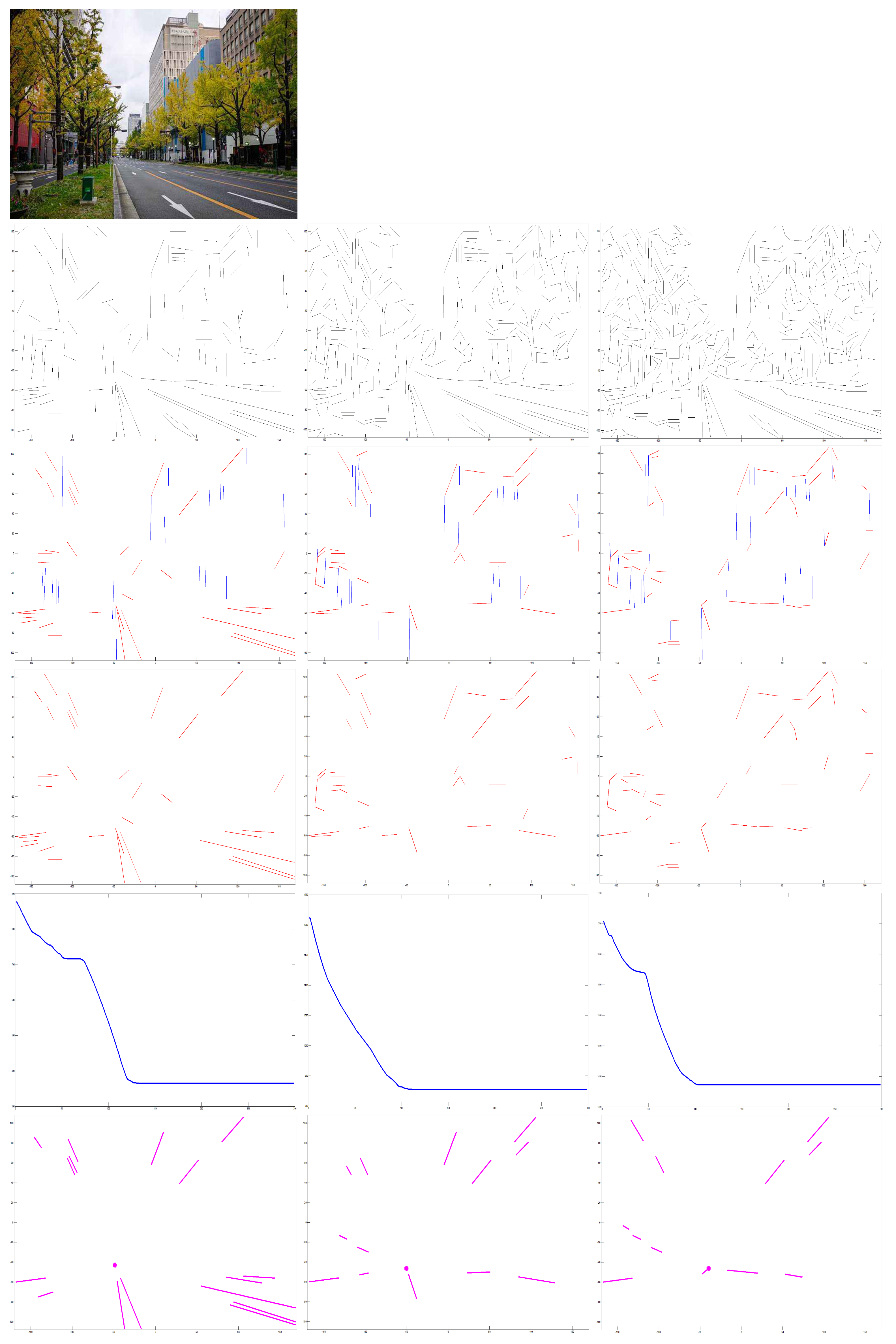
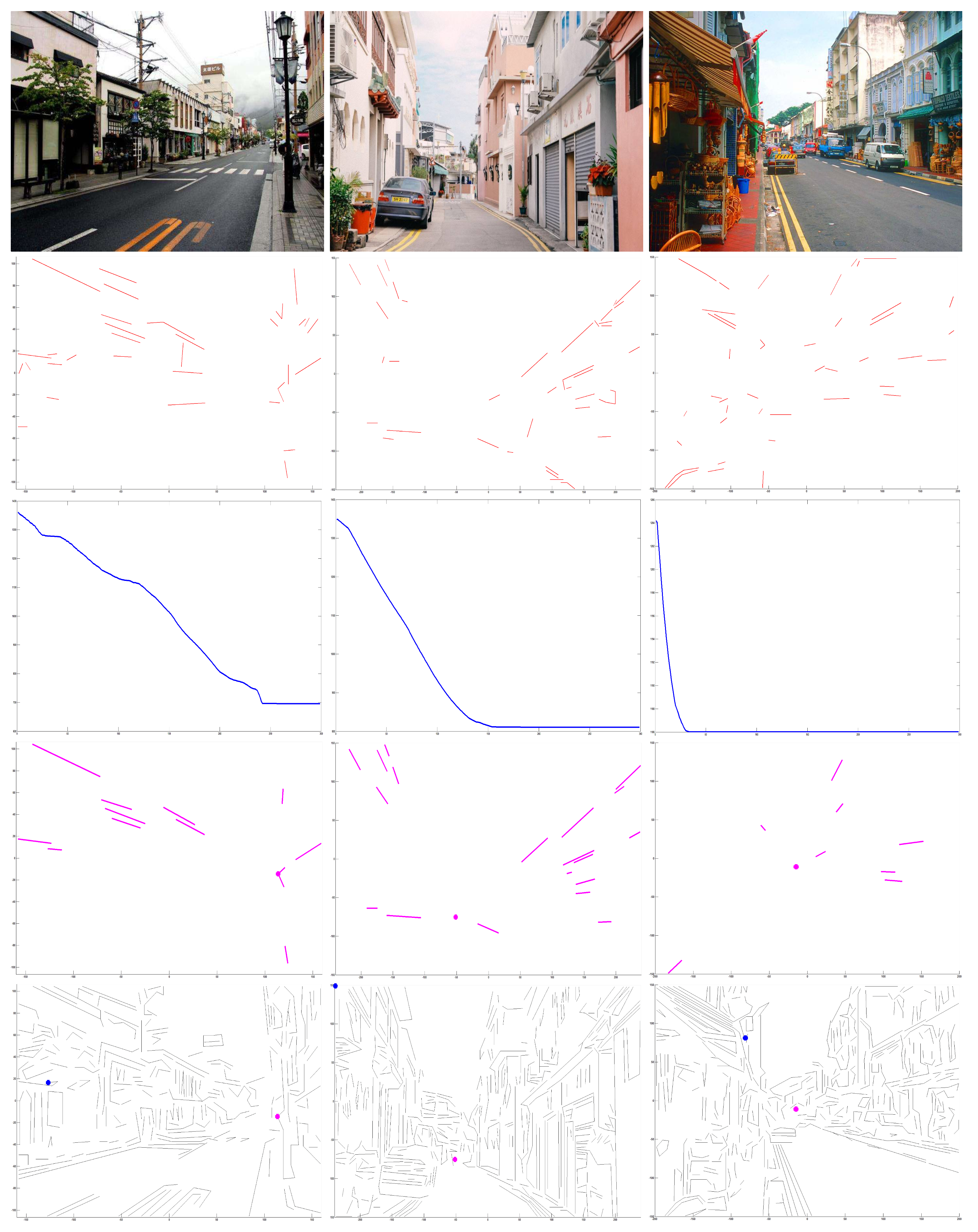
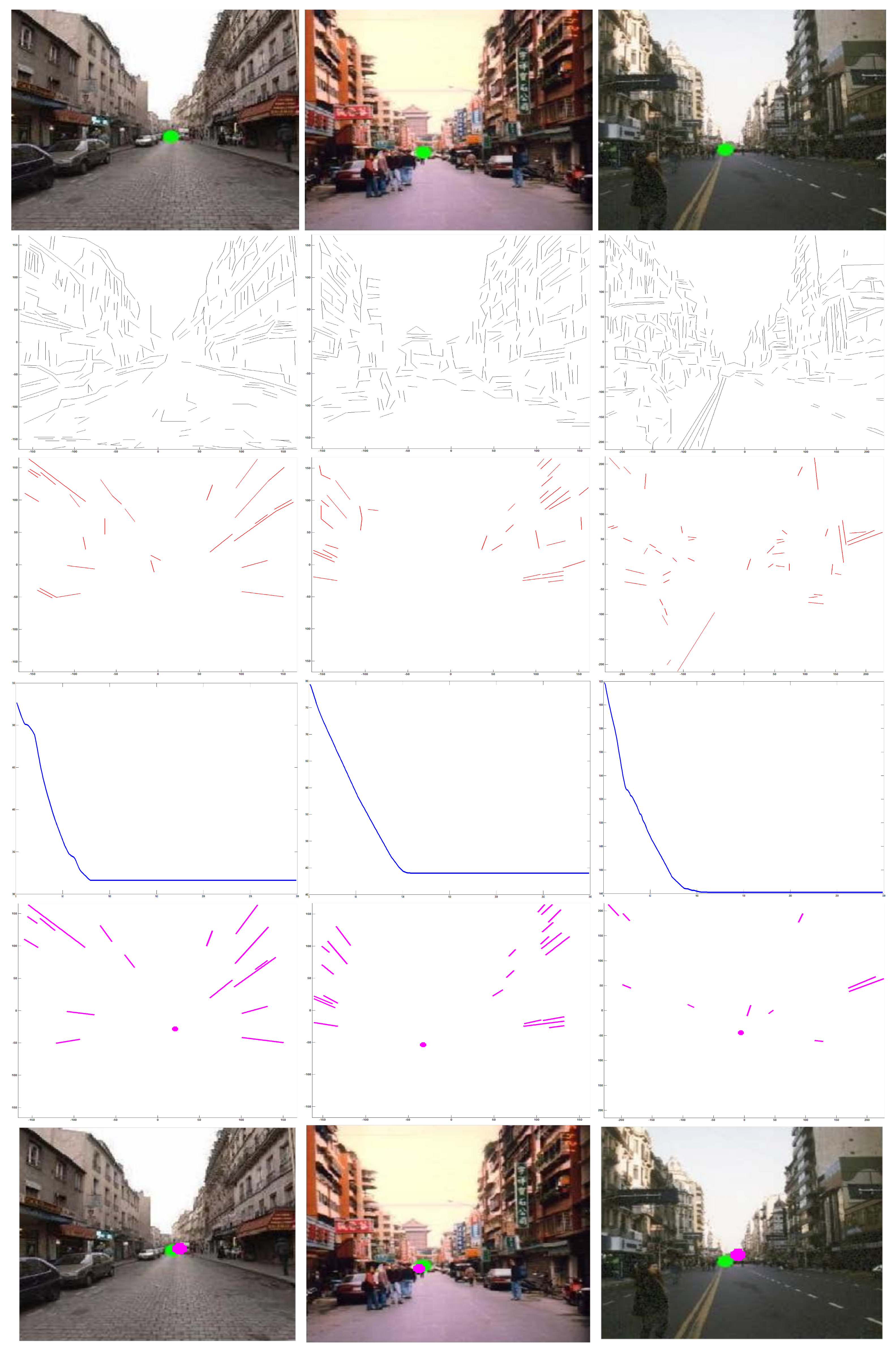
4. Experimental Results

4.1. Evaluation

In this paper, we use a geometric algorithm to estimate VPs based on refined lines without prior training or any precise depth data. Compared to deep-learning-based algorithms, our approach requires no additional high-performance GPU. Lines is the cornerstone of VPs estimation. An experiment was performed on FDWW dataset [3]. The pixel errors were evaluated by comparing the estimated VPs to the ground truth, as shown in

Table 1. Evaluation of estimating VPs on FDWW dataset [3].

Method	Error
H.W. [3]	8.65%
Our method	3.23%

. It is proved that the VP estimated by refined lines can be used to efficiently estimate the VP.

In addition, lines are the base of proposed algorithm. Therefore, experiments were performed on input captures from lines extracted by different edge lines detection. As shown in Figure 3, for an input capture (top row), edge lines in second row were extracted through growing detector parameters. The parameter ${\lambda }_l$ controls number of lines that are to be detected. Its initial range ${\lambda }_l\in [0,1]$. ${\lambda }_l=0$ represents that no detected lines and ${\lambda }_l=1$ means full lines are to be extracted. It shows that the method can cope with an unstable edge detector. With the increasing numbers of lines that were extracted, it is obvious that our approach is robust to estimate VP by refining lines for different detected lines.

4.2. Comparison

Here, the experimental comparison were performed between H.W.’s method [3] and our method. H.W.’s approach estimates VPs through projections of spatial rectangles in which four line segments are combined. Because H.W.’s approach just uses original lines, and it is short of the process of refining lines, it has difficulty in describing robust VPs when there are a amount of disturbance of varying illumination and color. By contrast, our methods is capable of estimating robust VPs in such scenarios, which is helpful in improving environment perception performance of vision-based vehicles, as shown in Figure 4.

More experimental comparison were performed between Hyeong’s method [14] and our algorithm. As shown in Figure 5, compared to the green point estimated by Hyeong’s method [14], our approach has a better estimation through refined lines.

The speed and consumption of VP estimation is a vital factor for automatic driving. The experiments were run on a computer with Intel Core i7-6500 2.50 GHZ CPU. The run-time for efficiency analysis of different methods, as shown in

Table 2. Average Time on FDWW dataset [3].

Method	Time (s)
Wei [3]	3.3
Our method	1.6

. Since Wei’s method estimates VPs by rectangles, it is time-consuming. Our approach contends geometrical inferences with refined lines that has lower numbers of lines, leading to less run time. The algorithm with low consumption and high efficiency looks promising, which is more practical for implementation in a autonomous vehicles.

5. Conclusions

The current work presents an geometric algorithm for autonomous vehicles to estimate VPs without any prior training from monocular vision. The edge lines were refined by structured configurations based on geometric constraints. Then, VPs can be obtained by optimal estimation from different clusters in refined lines. Unlike data-driven methods, the proposed approach requires no prior training. Compared to methods using only edge lines, the presented approach has better efficiency by adopting refined lines. Because geometric inferences was adopted, the proposed algorithm has ability to cope with varying illumination and color, which is more practical and efficient for scene understanding in autonomous driving. The percentage of pixel error by relative estimation were measured by comparing the estimated VPs to the ground truth. The results proved that the presented approach can estimate robust VPs, meeting the requirements of visual navigation in autonomous vehicles. Furthermore, the proposed refined-line strategy is based on original line detection, and an algorithm to extract lines from an image involving great disturbance of color and noise is to be developed in the future work.

References

- Gibson, E.J.; Walk, R.D. The visual cliff. Sci. Am. 1960, 202, 64–71. [Google Scholar] [CrossRef] [PubMed]
- Koenderink, J.J.; Doorn, A.J.V.; Kappers, A.M. Pictorial surface attitude and local depth comparisons. Percept. Psychophys. 1996, 58, 163–173. [Google Scholar] [CrossRef] [PubMed] [Green Version]
- Wang, H.W. Understanding of Indoor Scenes Based on Projection of Spatial Rectangles. Pattern Recognit. 2018, 81, 497–514. [Google Scholar]
- Wang, H.W.L. Visual Navigation Using Projection of Spatial Right-Angle In Indoor Environment. IEEE Trans. Image Process. (TIP) 2018, 27, 3164–3177. [Google Scholar]
- Wang, L.; Wei, H. Understanding of Curved Corridor Scenes Based on Projection of Spatial Right-Angles. IEEE Trans. Image Process. (TIP) 2020, 29, 9345–9359. [Google Scholar] [CrossRef] [PubMed]
- Masland, R. The fundamental plan of the retina. Nat. Neurosci. 2001, 4, 877–886. [Google Scholar] [CrossRef] [PubMed]
- Jonas, J.B.; Schneider, U.; Naumann, G.O. Count and density of human retinal photoreceptors. Graefe’s Arch. Clin. Exp. Ophthalmol. 1992, 230, 505–510. [Google Scholar] [CrossRef]
- Balasuriya, S.; Siebert, P. A biologically inspired computational vision frontend based on a self-organised pseudo-randomly tessellated artificial retina. In Proceedings of the IEEE Proceedings of the International Joint Conference on Neura Networks, Montreal, QC, Canada, 31 July–4 August 2005; pp. 3069–3074. [Google Scholar]
- Wei, H.; Li, J. Computational Model for Global Contour Precedence Based on Primary Visual Cortex Mechanisms. ACM Trans. Appl. Percept. (TAP) 2021, 18, 14:1–14:21. [Google Scholar] [CrossRef]
- Wang, H.W. A Visual Cortex-Inspired Imaging-Sensor Architecture and Its Application in Real-Time Processing. Sensors 2018, 18, 2116. [Google Scholar]
- Khaliluzzaman, M. Analytical justification of vanishing point problem in the case of stairways recognition. J. King Saud Univ.-Comput. Inf. Sci. 2021, 33, 161–182. [Google Scholar] [CrossRef]
- Jang, J.; Jo, Y.; Shin, M.; Paik, J. Camera Orientation Estimation Using Motion-Based Vanishing Point Detection for Advanced Driver-Assistance Systems. IEEE Trans. Intell. Transp. Syst. 2021, 22, 6286–6296. [Google Scholar] [CrossRef]
- Lopez-Martinez, A.; Cuevas, F.J. Vanishing point detection using the teaching learning-based optimisation algorithm. IET Image Process. 2020, 14, 2487–2494. [Google Scholar] [CrossRef]
- Yoon, G.J.; Yoon, S.M. Optimized Clustering Scheme-Based Robust Vanishing Point Detection. IEEE Trans. Intell. Transp. Syst. 2020, 21, 199–208. [Google Scholar]
- Simon, G.; Tabbone, S. Generic Document Image Dewarping by Probabilistic Discretization of Vanishing Points. In Proceedings of the 2020 25th International Conference on Pattern Recognition (ICPR), Milan, Italy, 10–15 January 2021; pp. 2344–2351. [Google Scholar]
- Garcia-Faura, A.; Fernandez-Martinez, F.; Kleinlein, R.; San-Segundo, R.; de Maria, F.D. A multi-threshold approach and a realistic error measure for vanishing point detection in natural landscapes. Eng. Appl. Artif. Intell. 2019, 85, 713–726. [Google Scholar] [CrossRef]
- Moon, Y.Y.; Geem, Z.W.; Han, G.T. Vanishing point detection for self-driving car using harmony search algorithm. Swarm Evol. Comput. 2018, 41, 111–119. [Google Scholar] [CrossRef]
- Lee, J.; Yoon, K. Joint Estimation of Camera Orientation and Vanishing Points from an Image Sequence in a Non-Manhattan World. Int. J. Comput. Vis. 2019, 127, 1426–1442. [Google Scholar] [CrossRef]
- Liu, Y.B.; Zeng, M.; Meng, Q.H. Unstructured Road Vanishing Point Detection Using Convolutional Neural Networks and Heatmap Regression. IEEE Trans. Instrum. Meas. 2021, 70, 1–8. [Google Scholar] [CrossRef]
- Lee, D.; Gupta, A.; Hebert, M.; Kanade, T. Estimating Spatial Layout of Rooms using Volumetric Reasoning about Objects and Surfaces. In Proceedings of the 23rd International Conference on Neural Information Processing Systems, Vancouver, BC, Canada, 6–9 December 2010; pp. 1288–1296. [Google Scholar]
- Wang, L.; Wei, H. Indoor scene understanding based on manhattan and non-manhattan projection of spatial right-angles. J. Vis. Commun. Image Represent. 2021, 80, 103307. [Google Scholar] [CrossRef]
- Pero, L.D.; Bowdish, J.; Fried, D.; Kermgard, B.; Hartley, E.; Barnard, K. Bayesian geometric modeling of indoor scenes. In Proceedings of the IEEE Computer Society Conference on Computer Vision and Pattern Recognition (CVPR), Providence, RI, USA, 16–21 June 2012; pp. 2719–2726. [Google Scholar]
- Wang, L.; Wei, H. Understanding of wheelchair ramp scenes for disabled people with visual impairments. Eng. Appl. Artif. Intell. 2020, 90, 103569. [Google Scholar] [CrossRef]
- Choi, H.S.; An, K.; Kang, M. Regression with residual neural network for vanishing point detection. Image Vis. Comput. 2019, 91, 103797. [Google Scholar] [CrossRef]
- Wang, L.; Wei, H. Avoiding non-Manhattan obstacles based on projection of spatial corners in indoor environment. IEEE/CAA J. Autom. Sin. 2020, 7, 1190–1200. [Google Scholar] [CrossRef]
- Wang, L.; Wei, H. Reconstruction for Indoor Scenes Based on an Interpretable Inference. IEEE Trans. Artif. Intell. 2021, 2, 251–259. [Google Scholar] [CrossRef]
- Khaliluzzaman, M.; Deb, K. Stairways detection based on approach evaluation and vertical vanishing point. Int. J. Comput. Vis. Robot. 2018, 8, 168–189. [Google Scholar] [CrossRef]
- Han, J.; Yang, Z.; Hu, G.; Zhang, T.; Song, J. Accurate and Robust Vanishing Point Detection Method in Unstructured Road Scenes. J. Intell. Robot. Syst. 2019, 94, 143–158. [Google Scholar] [CrossRef]
- Wang, E.; Sun, A.; Li, Y.; Hou, X.; Zhu, Y. Fast vanishing point detection method based on road border region estimation. IET Image Process. 2018, 12, 361–373. [Google Scholar] [CrossRef]
- Tarrit, K.; Molleda, J.; Atkinson, G.A.; Smith, M.L.; Wright, G.C.; Gaal, P. Vanishing point detection for visual surveillance systems in railway platform environments. Comput. Ind. 2018, 98, 153–164. [Google Scholar] [CrossRef]
- Wang, L.; Wei, H. Curved Alleyway Understanding Based on Monocular Vision in Street Scenes. IEEE Trans. Intell. Transp. Syst. 2021, 1–20. [Google Scholar] [CrossRef]
- Nagy, T.K.; Costa, E.C.M. Development of a lane keeping steering control by using camera vanishing point strategy. Multidimens. Syst. Signal Process. 2021, 32, 845–861. [Google Scholar] [CrossRef]
- Wang, H.W.D. V4 shape features for contour representation and object detection. Neural Netw. 2017, 97, 46–61. [Google Scholar]
- Arbelaez, P.; Maire, M.; Fowlkes, C. From contours to regions: An empirical evaluation. In Proceedings of the IEEE Computer Society Conference on Computer Vision and Pattern Recognition (CVPR), Miami, FL, USA, 20–25 June 2009; pp. 2294–2301. [Google Scholar]
- Wei, H.; Wang, L.; Wang, S.; Jiang, Y.; Li, J. A Signal-Processing Neural Model Based on Biological Retina. Electronics 2020, 9, 35. [Google Scholar] [CrossRef] [Green Version]
- Kennedy, J.; Eberhart, R. Particle swarm optimization. In Proceedings of the IEEE International Conference on Neural Networks, Perth, WA, Australia, 27 November–1 December 1995; pp. 1942–1948. [Google Scholar]
Publisher’s Note: MDPI stays neutral with regard to jurisdictional claims in published maps and institutional affiliations. |
© 2022 by the authors. Licensee MDPI, Basel, Switzerland. This article is an open access article distributed under the terms and conditions of the Creative Commons Attribution (CC BY) license (https://creativecommons.org/licenses/by/4.0/).
Share and Cite
Shen, S.; Wang, S.; Wang, L.; Wei, H. A Refined-Line-Based Method to Estimate Vanishing Points for Vision-Based Autonomous Vehicles. Vehicles 2022, 4, 314-325. https://doi.org/10.3390/vehicles4020019
Shen S, Wang S, Wang L, Wei H. A Refined-Line-Based Method to Estimate Vanishing Points for Vision-Based Autonomous Vehicles. Vehicles. 2022; 4(2):314-325. https://doi.org/10.3390/vehicles4020019
Chicago/Turabian StyleShen, Shengyao, Shanshan Wang, Luping Wang, and Hui Wei. 2022. "A Refined-Line-Based Method to Estimate Vanishing Points for Vision-Based Autonomous Vehicles" Vehicles 4, no. 2: 314-325. https://doi.org/10.3390/vehicles4020019